On Neighborhood Inverse Sum Indeg Energy of Molecular Graphs

Abstract

The spectral graph theory explores connections between combinatorial features of graphs and algebraic properties of associated matrices. The neighborhood inverse sum indeg ($NI$) index was recently proposed and explored to be a significant molecular descriptor. Our aim is to investigate the $NI$ index from a spectral standpoint, for which a suitable matrix is proposed. The matrix is symmetric since it is generated from the edge connection information of undirected graphs. A novel graph energy is introduced based on the eigenvalues of that matrix. The usefulness of the energy as a molecular structural descriptor is analyzed by investigating predictive potential and isomer discrimination ability. Fundamental mathematical properties of the present spectrum and energy are investigated. The spectrum of the bipartite class of graphs is identified to be symmetric about the origin of the real line. Bounds of the spectral radius and the energy are explained by identifying the respective extremal graphs.

1. Introduction

Throughout this paper, we consider finite, simple, and undirected graphs. Let G be a graph of order n and size m whose node and edge sets are $V\left(G\right)$ and $\mathcal{E}\left(G\right)$, respectively. If two nodes $v_i$, $v_j$ are linked by an edge, then we represent it as $v_i{v}_j\in \mathcal{E}\left(G\right)$. By $N_G\left(v_i\right)$ we mean the set of vertices connected to $v_i$ (i.e., neighbors of $v_i$). Clearly, the degree of a node $v_i$, denoted as $d_i$ is equal to $|N_G\left(v_i\right)|$. Let ${\delta }_i={\displaystyle \sum _{v_i{v}_j\in \mathcal{E}\left(G\right)}}{d}_j$. We refer to ${\delta }_i$ as the neighborhood degree sum of $v_i$.

Topological indices are numerical quantities derived from the molecular graph that remain invariant for isomorphic graphs. Hundreds of topological indices have been proposed and researched in the literature of mathematical chemistry due to their extensive applications in structure–property and structure–activity modeling, beginning in 1947 when the distance-based Wiener index was found to model the boiling point of paraffin [1]. The journey of degree-based indices was started through Zagreb indices [2] to provide quantitative measures of molecular branching, which led to a significant variety of such useful indices [3]. The goal of designing a novel descriptor is to obtain higher accuracy in modeling molecular properties than previously available descriptors. Due to significant impact in describing various features of molecule, researchers are paying close attention to neighborhood degree sum-based descriptors [4,5,6,7,8,9]. Their application potential in predicting the physico-chemical properties of molecule and isomer discrimination are investigated in [10,11,12]. The neighborhood inverse sum indeg ($NI$) index is one such descriptor, which appeared in 2019 [13] but was established as an effective structural descriptor in 2020 [12]. Its formulation is as follows:

$$\begin{array}{c}\hfill NI\left(G\right)=\sum _{v_i{v}_j\in \mathcal{E}\left(G\right)}\frac{{\delta }_i{\delta }_j}{{\delta }_i+{\delta }_j}.\end{array}$$

Spectral graph theory [14] is an attractive research area that finds the relation between the combinatorial properties of graphs and the algebraic properties of associated matrices, as well as applications of those connections. More broadly, it searches for the link between the discrete universe and the continuous one by employing geometric, analytic, and algebraic techniques. For a graph G, the conventional adjacency matrix, denoted as $A\left(G\right)$, is one of the effective tools in this domain. The $(i,j)$-element of $A\left(G\right)$ is 1 when $v_i{v}_j\in \mathcal{E}\left(G\right)$, and 0 elsewhere. Its characteristic polynomial is ${\Psi }_A(G,\lambda )=det(\lambda I_n-A\left(G\right))$, where $I_n$ is the identity matrix. Since $A\left(G\right)$ is real and symmetric, one can arrange its eigenvalues as ${\lambda }_1\ge {\lambda }_2\ge \cdots \ge {\lambda }_n$. The multiset $\{{\lambda }_1,{\lambda }_2,\dots ,{\lambda }_n\}$ is known as the A-spectrum of G, which is referred to as $Sp\left(A\right(G\left)\right)$. Gutman initiated an excellent research direction based on the A-spectrum in 1978 when he introduced graph energy [15], which was gradually recognized, and now it occupies a massive area in mathematical chemistry and algebraic graph theory. Initially, it was found to explain the total $\pi$-electron energy, and it was later established as a significant molecular structure descriptor [16,17,18]. The energy $E\left(G\right)$ is the sum of absolute A-eigenvalues of G. A significant amount of research has been conducted on this idea [16]. Following the potential applications of the A-spectrum, numerous topological indices were investigated from a spectral perspective by modifying the classical adjacency matrix accordingly [19,20,21,22,23,24,25,26,27,28,29]. Zhou and Trinajstić [30] introduced the matrix corresponding to the sum-connectivity index and studied associated energy in 2010. In 2015, Rodriguez and Sigarreta [31,32] investigated the spectral properties of the geometric–arithmetic index. Mondal et al. [33] presented chemical significance of some eigenvalue-based indices. In 2018, Rad et al. [34] introduced the Zagreb energy and derived its crucial bounds with characterizing extremal graphs. The spectral behavior of the Sombor index was recently reported in [35]. The spectral properties of inverse sum indeg ($ISI$) index were recently studied [36,37] for which the $ISI$ matrix was defined, whose $(i,j)$-element is $\frac{d_i{d}_j}{d_i+d_j}$ when $v_i{v}_j\in \mathcal{E}\left(G\right)$, and 0 otherwise. Usually, the inverse sum indeg energy ($E_{ISI}$) is defined as the sum of absolute eigenvalues of the $ISI$ matrix. Interesting mathematical features of $E_{ISI}$ were explored by Hafeez and Farooq [38]. Recently, Ye and Li [39] identified equienergetic graphs with respect to $E_{ISI}$. The major goal of the present work is to study the $NI$ index in a spectral approach. Our main tool for such investigation is an appropriate matrix, named $NI$-matrix, denoted by $A_{NI}\left(G\right)$, whose $(i,j)$-entry is as follows:

$$a_{ij}=\left\{\begin{array}{c}\frac{{\delta }_i{\delta }_j}{{\delta }_i+{\delta }_j}if{v}_i{v}_j\in \mathcal{E}\left(G\right),\hfill \\ 0otherwise.\hfill \end{array}\right.$$

The $NI$-characteristic polynomial of G is expressed as ${\Psi }_{NI}(G,\rho )=det(\rho I_n-A_{NI}\left(G\right))$. Let $\{{\rho }_1,{\rho }_2,\dots ,{\rho }_n\}$ be the complete list of roots of ${\Psi }_{NI}(G,\rho )=0$. Since $A_{NI}\left(G\right)$ is real and symmetric, ${\rho }_i$ are also real and we can arrange them in non-increasing order as ${\rho }_1\ge {\rho }_2\ge \cdots \ge {\rho }_n$. The collection $\{{\rho }_1,{\rho }_2,\dots ,{\rho }_n\}$ is termed as $NI$-spectrum of G, and is represented by $Sp\left(A_{NI}\left(G\right)\right)$. We call ${\rho }_1$ the $NI$-spectral radius of G. In accordance with the general concepts by which the energy idea is adapted to different graph-theoretical matrices, the neighborhood inverse sum indeg energy ($E_{NI}$) is defined as

$$\begin{array}{c}\hfill E_{NI}\left(G\right)=\sum _{i=1}^n\left|{\rho }_i\right|.\end{array}$$

The main focus of this research is to explore the chemical significance of the $E_{NI}$ energy and to demonstrate crucial mathematical attributes of the $NI$-spectral radius and $E_{NI}$ energy. The $NI$-spectrum is observed to be symmetric about the origin for the bipartite graph. We will now describe some terms and symbols that will be utilized all through the paper. For minimum and maximum degrees, we use $\delta$ and $\Delta$, respectively. If $d_u=r$$\forall u\in V\left(G\right)$ and for some natural number r, then G is known as r-regular. To represent the path, cycle, star and complete graphs having n nodes, we consider $P_n$, $C_n$, $S_n$ and $K_n$, respectively. Let G be bipartite with the partition of the node set as $V\left(G\right)=V_1\cup V_2$. If $|V_1|=\alpha$, $|V_2|=\beta$ and all nodes belonging to the same node set have equal degree, then G is known as $(\alpha ,\beta )$-semiregular bipartite. We use $K_{p,q}$ to represent the complete bipartite graph whose vertices are partitioned into two sets having $p,q$ nodes. To represent strongly regular graph of order n, we consider $G_s(n,r,\sigma ,\tau )$. It is an r regular graph having the following property: if $v_i{v}_j\in \mathcal{E}\left(G_s(n,r,\sigma ,\tau )\right)$, then $|N_G\left(v_i\right)\cap N_G\left(v_j\right)|=\sigma$, else $|N_G\left(v_i\right)\cap N_G\left(v_j\right)|=\tau$.

We can construct the remaining portion of the report in the following manner. The following section explains the pseudocode that can be used to expedite the computation. The contributions of $E_{NI}$ and $E_{ISI}$ as molecular structural descriptors are examined in Section 3. In Section 4, crucial bounds for the $NI$-spectral radius are evaluated by recognizing the graphs for which the bound attains. In Section 5, the bounds of $E_{NI}$ energy are computed. With some decisive remarks, the paper is concluded in Section 6.

2. Computational Methodology

A MATLAB code is developed to compute the energy in an efficient manner, the algorithm for that is described here (see Algorithm 1). In MATLAB, the declaration of variables is not needed. We used S and $\Gamma$ to contain the $ISI$ and $NI$ matrices, respectively. To store the degree and neighborhood degree sum of nodes, d, and $NDS$ are considered, respectively. The $ISI$ and $NI$ spectrum are stored in $e_1$ and $e_2$, respectively.

Algorithm 1 Computational procedure of $ISI$-spectrum, $NI$-spectrum, $E_{ISI}$ and $E_{NI}$ energies.

Input: Edge connection of $G=(V,E)$ and order of G. Output: $ISI$-spectrum, $NI$-spectrum, $E_{ISI}$ and $E_{NI}$ energy. Step 1. Start. Step 2. Read Edge connection of G, $\left|V\right|$. Step 3. Set S, $A_N$, $\Gamma$ to zero matrix of order $\left|V\right|$. Step 4. A← Adjacency matrix of G Step 5. d← vertex degree of G Step 6. Construct S: for$i=1to\left|V\right|$do     for $j=1to\left|V\right|$ do         if $A(i,j)=1$ then            $S(i,j)$←$\frac{d\left(i\right)d\left(j\right)}{d\left(i\right)+d\left(j\right)}$         end if     end for end for Step 7. $e_1$← eigenvalues of S Step 8. $E_{ISI}$← summation of absolute $e_1$ Step 9. Construct $A_N$: for$i=1to\left|V\right|$do     for $j=1to\left|V\right|$ do         if $i=j$ then            $A_N(i,j)\leftarrow -d{\left(i\right)}^2$         else if $A(i,j)=1$ then            $A_N(i,j)\leftarrow d\left(i\right)+d\left(j\right)$         end if     end for end for Step 10. $NDS$← row sum of $A_N$ Step 11. Construct $\Gamma$: for$i=1to\left|V\right|$do     for $j=1to\left|V\right|$ do         if $A(i,j)=1$ then            $\Gamma (i,j)$←$\frac{NDS\left(i\right)NDS\left(j\right)}{NDS\left(i\right)+NDS\left(j\right)}$         end if     end for end for Step 12. $e_2$← eigenvalues of $\Gamma$ Step 13. $E_{NI}$← summation of absolute $e_2$ Step 14. Stop.

To examine the predictive capability of the energies, linear regression models are built. The statistical parameters are generated by MATLAB and excel statistical functions. The graphical representations are made using the MATLAB plotting library. The external validation of derived models is performed using Python sklearn and the Pandas library on Jupiter notebook IDE.

3. Significance as Structural Descriptor

A great variety of graph energy variants have been proposed in the literature to date [16,21,30,31,32,34]. The majority of these were introduced haphazardly, with no motivation or attempt to apply the novel energy in chemistry (or anywhere else). The present work is a happy exception to this trend. The inverse sum indeg energy was first presented by Zangi et al. [37] and some mathematical study of that energy was later performed in [36,38]. However, no attention was paid to investigating the role of $E_{ISI}$ as a regulator of molecular properties. Here, we aim to examine the acceptability of $E_{ISI}$, $E_{NI}$ energies as potential structural descriptors. To assess the chemical significance of a graph invariant, the invariant should always be correlated with the experimental properties of a benchmark data set. We perform regression analysis considering two types of data sets: octane isomers and benzenoid hydrocarbons. The theoretical values of the energies for chemical compounds are computed by means of in-house MATLAB code. The experimental properties of octanes [11,40,41] are correlated with $E_{ISI}$ and $E_{NI}$ energies. Unfortunately, no notable correlation is found for both energies. To enhance the skill of these energies in modeling physico-chemical properties, we devise a linear model:

$$\begin{array}{c}\hfill E_{ISI}+k{E}_{NI},\end{array}$$

(1)

where k is the fitting parameter running from −20 to 20. Surprisingly, a major improvement is found when the model (1) is correlated with different properties of octanes. We propose to investigate the following model:

$$\begin{array}{c}\hfill Y=I(\pm 2S_e)+J(\pm 2S_e)M_d.\end{array}$$

(2)

In the above model, $Y,I,S_e,J$ and $M_d$ denote property, intercept, standard error of coefficients, slope, and molecular descriptor, respectively. In addition to the model (2), we intend to examine some more parameters, such as the correlation coefficient (r), standard error of the model ($SE$), the F-test (F), and the significance F ($SF$). The regression equations for model (1) by the relation (2) are as follows:

$$\begin{array}{c}\hfill DHVAP=6.2093(\pm 0.3938)+0.6714(\pm 0.0899)(E_{ISI}-0.2E_{NI}),\\ \hfill r^2=0.9329,SE=0.1023,F=222.7995,SF=8.22\times {10}^{-11}.\end{array}$$

(3)

$$\begin{array}{c}\hfill Acentricfactor=0.4389(\pm 0.012)+0.0408(\pm 0.0045)(E_{ISI}-0.6E_{NI}),\\ \hfill r^2=0.9534,SE=0.0079,F=326.9797,SF=4.5\times {10}^{-12}.\end{array}$$

(4)

$$\begin{array}{c}\hfill S=118.3899(\pm 1.8907)+5.1383(\pm 0.7118)(E_{ISI}-0.6E_{NI}),\\ \hfill r^2=0.9287,SE=1.2433,F=208.4465,SF=1.35\times {10}^{-10}.\end{array}$$

(5)

$$\begin{array}{c}\hfill HVAP=45.6946(\pm 3.6149)+3.8715(\pm 0.5944)(E_{ISI}-0.1E_{NI}),\\ \hfill r^2=0.9138,SE=0.6131,F=169.6805,SF=6.21\times {10}^{-10}.\end{array}$$

(6)

$$\begin{array}{c}\hfill bp=20.0287(\pm 20.5721)+12.0411(\pm 2.6399)(E_{ISI}+0E_{NI}),\\ \hfill r^2=0.8387,SE=2.532,F=83.215,SF=9.71\times {10}^{-8}.\end{array}$$

(7)

$$\begin{array}{c}\hfill CT=67.7833(\pm 68.0764)+17.1578(\pm 5.2607)(E_{ISI}+0.3E_{NI}),\\ \hfill r^2=0.7267,SE=5.2473,F=42.5488,SF=7.02\times {10}^{-6}.\end{array}$$

(8)

Ramane et al. [42] explored the linear dependence of $\pi$-electron energy ($E_{\pi }$) on some degree-based descriptors for benzenoid hydrocarbons. We correlated the $E_{ISI}$ and $E_{NI}$ energies with the same attribute for the same set of hydrocarbons. Now in view of (2), the following models are generated for benzenoid hydrocarbons:

$$\begin{array}{c}\hfill E_{\pi }=2.1229(\pm 0.8591)+0.7831(\pm 0.0248)E_{ISI},\\ \hfill r^2=0.993,SE=0.6037,F=3975.569,SF=1\times {10}^{-31}.\end{array}$$

(9)

$$\begin{array}{c}\hfill E_{\pi }=3.6909(\pm 1.0089)+0.2959(\pm 0.0117)E_{NI},\\ \hfill r^2=0.9892,SE=0.7496,F=2568.963,SF=4.31\times {10}^{-29}.\end{array}$$

(10)

We have correlated the $E_{ISI}$ and $E_{NI}$ energies with bp for the set of benzenoid hydrocarbons used by Ramane and Yalnaik [43] also for distance-based descriptors. In view of Equation (2), the following models for bp are obtained.

$$\begin{array}{c}\hfill bp=36.1728(\pm 23.5537)+13.3853(\pm 0.6798)E_{ISI},\\ \hfill r^2=0.9879,SE=11.2788,F=1550.857,SF=1.11\times {10}^{-19}.\end{array}$$

(11)

$$\begin{array}{c}\hfill bp=75.0229(\pm 38.2081)+4.9291(\pm 0.4425)E_{NI},\\ \hfill r^2=0.9631,SE=19.6865,F=496.2889,SF=4.45\times {10}^{-15}.\end{array}$$

(12)

When we go through the models (3)–(12), several interesting remarks can be drawn. The lower the $Se$ values, the more certain one can be about the regression model. The models (3), (4), (6), (9) and (10) have very small $SE$. The models (9) and (10) have remarkably good F-values. A model is considered statistically reliable when the $SF$ value is less than 0.05. Each of the models yields $SF$ that is considerably lower than 0.05. The variations of absolute correlation coefficients ($\left|r\right|$) of the model (1) for varying k are depicted in Figure 1, Figure 2 and Figure 3. The solid blue line represents the variation of $\left|r\right|$ values with k. The dashed red and green lines indicate the $\left|r\right|$ values of $E_{ISI}$ and $E_{NI}$, respectively, for respective properties.

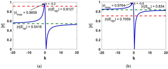
Figure 1. Plotting of $\left|r\right|$ versus k for (a) DHVAP and (b) AF of octanes.

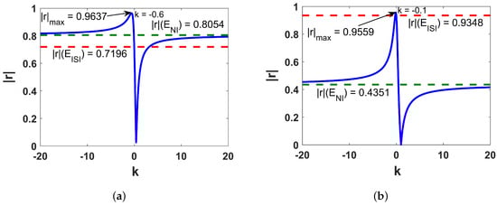
Figure 2. Plotting of $\left|r\right|$ versus k for (a) S and (b) HVAP of octanes.

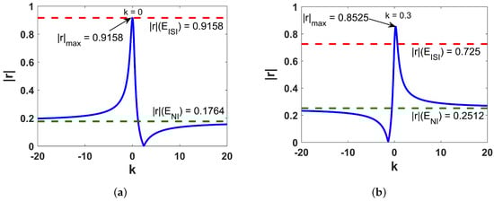
Figure 3. Plotting of $\left|r\right|$ versus k for (a) bp and (b) CT of octanes.

From Figure 1, Figure 2 and Figure 3, it is apparent that the individual contributions of $E_{ISI}$ and $E_{NI}$ in predicting different physico-chemical properties are not satisfactory, but their linear combination (1) reaches a sharp maximum for standard enthalpy of vaporization (DHVAP), acentric factor (AF), entropy (S), enthalpy of vaporization (HVAP) and heat capacity at T constant (CT) at $k=-0.2,-0.6,-0.6,-0.1,0.3$, respectively. For bp, the red line touches the maximum point of the blue line at $k=0$. Correlation of $E_{\pi }$ with $E_{ISI}$ and $E_{NI}$ for benzenoid hydrocarbons is shown in Figure 4. The $\left|r\right|$ for both of them are significantly high, in fact, quite close to the optimal value.

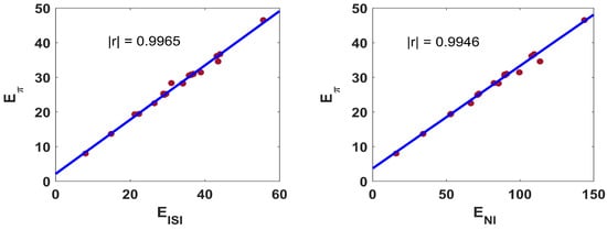
Figure 4. Correlation of $E_{ISI}$ and $E_{NI}$ with $E_{\pi }$ for 30 benzenoid hydrocarbons.

The correlation of $E_{ISI}$ and $E_{NI}$ with $bp$ for benzenoid hydrocarbons is shown in Figure 5. The efficacy of both of them is remarkable in predicting $bp$, outperforming the distance-based invariants reported on [43].

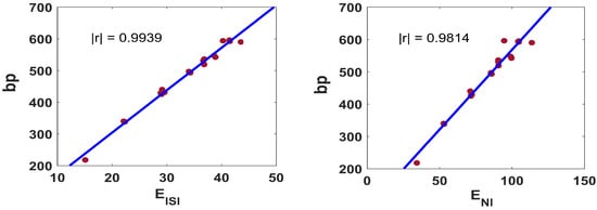
Figure 5. Correlation of $E_{ISI}$ and $E_{NI}$ with $bp$ for 21 benzenoid hydrocarbons.

Our models performed well in terms of accuracy; however, external validation is essential to truly evaluate the predictability of models. For this, we consider the nonane isomers of 35 compounds. Since the model (1) yields the best performance in describing the acentric factor of octanes, we decide to perform external validation for $AF$. The experimental values of $AF$ are collected from the chemical database [44]. Using the Python sklearn library, the data collection is randomly split into training ($80\%$) and test ($20\%$) sets. The training set produces the following model (13) fitting parameters, which reveal significant predictive potential. The linear fitting of model (13) is depicted in Figure 6a.

$$\begin{array}{c}\hfill Acentricfactor=0.4983(\pm 0.0218)+0.0449(\pm 0.0068)(E_{ISI}-0.6E_{NI}),\\ \hfill r^2=0.8693,SE=0.0142,F=172.8753,SF=5.39\times {10}^{-13}.\end{array}$$

(13)

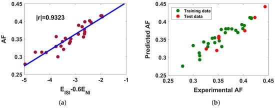
Figure 6. (a) Linear fitting of $AF$ with the model (1) for training set; (b) correlation between experimental and predicted $AF$.

The accuracy of the model (13) is found to be $90\%$ for the test set, which assures that our model is in good agreement with the experimental data. The relation between experimental and predicted acentric factors is shown graphically in Figure 6b. The correlation of $E_{ISI}$ and $E_{NI}$ with the boiling point of benzenoid hydrocarbons are found to be quite strong; however, when examined with external data, no meaningful outcome is observed.

The ultimate focus of a molecular descriptor is to estimate structure–property/structure–activity relationships. However, in order to encrypt as many structural characteristics of a molecule as possible, one well-descriptor should distinctively categorize each graph. The majority of descriptors have the disadvantage of producing the same descriptor for different isomers. Such a flaw is called degeneracy. The measure of degeneracy [45], known as sensitivity, is defined as

$$\begin{array}{c}\hfill S_d=\frac{N-N_d}{N}.\end{array}$$

If $\mathcal{C}$ is the collection of all considered isomers, then $N=\left|\mathcal{C}\right|$. By $N_d$, we mean that the descriptor is incapable of discriminating $N_d$ elements belonging to $\mathcal{C}$. A descriptor’s potential to discriminate between isomers is directly proportional to $S_d$. The $S_d$ of some mostly used descriptors are reported in [10] that ranges from 0.333 to 0.889. The $E_{ISI}$ and $E_{NI}$ energies, on the other hand, exhibit very good isomer discriminatory strength, having $S_D=1$. Consequently, the present energies perform better than existing descriptors in isomer discrimination. To examine how $E_{ISI}$ and $E_{NI}$ are independent, correlation among $E_{ISI}$, $E_{NI}$, E, Laplacian energy ($LE$) and the Estrada index ($EE$) is obtained in Table 1. It yields that $E_{NI}$ is independent among five invariants reported in Table 1, as $\left|r\right|$ for $E_{NI}$ is remarkably lower than others.

Table 1. Correlation coefficients among $E_{ISI}$, $E_{NI}$, E, $LE$ and $EE$.

	${\mathit{E}}_{\mathit{ISI}}$	${\mathit{E}}_{\mathit{NI}}$	E	$\mathit{LE}$	$\mathit{EE}$
$E_{ISI}$	1
$E_{NI}$	−0.258	1
E	0.988	−0.2736	1
$LE$	−0.7641	0.7729	−0.785	1
$EE$	−0.8041	0.7705	−0.8036	0.9386	1

4. Bounds for $\mathit{NI}$-Spectral Radius

Consider ${\mathcal{N}}_p$ as the p-th spectral moment of $A_{NI}=A_{NI}\left(G\right)$, for a graph G, i.e., ${\mathcal{N}}_p={\displaystyle \sum _{i=1}^n}{\left({\rho }_i\right)}^p$, where $p\in \mathbb{N}$. It is clear that ${\mathcal{N}}_p=Tr\left(A_{NI}^p\right)$. For convenience, the $NI$ value of an edge $v_i{v}_j$ is formulated as

$$\begin{array}{c}\hfill N{I}_G\left(v_i{v}_j\right)=\frac{{\delta }_i{\delta }_j}{{\delta }_i+{\delta }_j}.\end{array}$$

After performing some straightforward derivations on the entries of $A_{NI}$, we obtain the following result:

Lemma 1.

For a graph G with n nodes, we have

(i) 

${\mathcal{N}}_0=n$,

(ii) 

${\mathcal{N}}_1=0$,

(iii) 

${\mathcal{N}}_2=2{\displaystyle \sum _{v_i{v}_j\in \mathcal{E}\left(G\right)}}N{I}_G{\left(v_i{v}_j\right)}^2$,

(iv) 

${\mathcal{N}}_3=2{\displaystyle \sum _{\begin{array}{c}{v}_i{v}_j\in \mathcal{E}\left(G\right)\end{array}}}\left(N{I}_G\left(v_i{v}_j\right){\displaystyle \sum _{\begin{array}{c}{v}_i{v}_k,v_k{v}_j\in \mathcal{E}\left(G\right)\end{array}}}N{I}_G\left(v_i{v}_k\right)N{I}_G\left(v_k{v}_j\right)\right)$,

(v) 

${\mathcal{N}}_4={\displaystyle \sum _{v_i\in V\left(G\right)}}{\left({\displaystyle \sum _{\begin{array}{c}{v}_j\in V\left(G\right)\\ v_i{v}_j\in \mathcal{E}\left(G\right)\end{array}}}N{I}_G{\left(v_i{v}_j\right)}^2\right)}^2+{\displaystyle \sum _{v_i\ne v_j}}{\left({\displaystyle \sum _{\begin{array}{c}{v}_k\in V\left(G\right)\\ v_i{v}_k,v_k{v}_j\in \mathcal{E}\left(G\right)\end{array}}}N{I}_G\left(v_i{v}_k\right)N{I}_G\left(v_k{v}_j\right)\right)}^2$.

Proof. 

Results (i), (ii) and (iii) directly follow from the construction of $A_{NI}$. We prove parts (iv) and (v). For $i\ne j$, we have

$$\begin{array}{ccc}\hfill {\left(A_{NI}^2\right)}_{ij}& =& \sum _{v_k\in V\left(G\right)}N{I}_G\left(v_i{v}_k\right)N{I}_G\left(v_k{v}_j\right)={\displaystyle \sum _{\begin{array}{c}{v}_k\in V\left(G\right)\\ v_i{v}_k,v_k{v}_j\in \mathcal{E}\left(G\right)\end{array}}}N{I}_G\left(v_i{v}_k\right)N{I}_G\left(v_k{v}_j\right).\hfill \end{array}$$

Note that,

$$\begin{array}{ccc}\hfill {\left(A_{NI}^3\right)}_{ii}& =& \sum _{v_j\in V\left(G\right)}N{I}_G\left(v_i{v}_j\right){\left(A_{NI}^2\right)}_{ji}={\displaystyle \sum _{\begin{array}{c}{v}_j\in V\left(G\right)\\ v_i{v}_j\in \mathcal{E}\left(G\right)\end{array}}}\left(N{I}_G\left(v_i{v}_k\right){\displaystyle \sum _{\begin{array}{c}{v}_k\in V\left(G\right)\\ v_i{v}_k,v_k{v}_j\in \mathcal{E}\left(G\right)\end{array}}}N{I}_G\left(v_i{v}_k\right)N{I}_G\left(v_k{v}_j\right)\right).\hfill \end{array}$$

Thus, we obtain

$$\begin{array}{ccc}\hfill {\mathcal{N}}_3& =& \sum _{v_i\in V\left(G\right)}{\left(A_{NI}^3\right)}_{ii}\hfill \\ & =& \sum _{v_i\in V\left(G\right)}\left({\displaystyle \sum _{\begin{array}{c}{v}_j\in V\left(G\right)\\ v_i{v}_j\in \mathcal{E}\left(G\right)\end{array}}}\left(N{I}_G\left(v_i{v}_k\right){\displaystyle \sum _{\begin{array}{c}{v}_k\in V\left(G\right)\\ v_i{v}_k,v_k{v}_j\in \mathcal{E}\left(G\right)\end{array}}}N{I}_G\left(v_i{v}_k\right)N{I}_G\left(v_k{v}_j\right)\right)\right)\hfill \\ & =& 2{\displaystyle \sum _{\begin{array}{c}{v}_i{v}_j\in \mathcal{E}\left(G\right)\end{array}}}\left(N{I}_G\left(v_i{v}_j\right){\displaystyle \sum _{\begin{array}{c}{v}_i{v}_k,v_k{v}_j\in \mathcal{E}\left(G\right)\end{array}}}N{I}_G\left(v_i{v}_k\right)N{I}_G\left(v_k{v}_j\right)\right)\hfill \end{array}$$

Hence, part (iv) is done.

Now, we have

$$\begin{array}{ccc}\hfill {\mathcal{N}}_4& =& \sum _{v_i,v_j\in V\left(G\right)}{\left({\left(A_{NI}^2\right)}_{ij}\right)}^2=\sum _{i=j}{\left({\left(A_{NI}^2\right)}_{ij}\right)}^2+\sum _{i\ne j}{\left({\left(A_{NI}^2\right)}_{ij}\right)}^2\hfill \\ & =& {\displaystyle \sum _{v_i\in V\left(G\right)}}{\left({\displaystyle \sum _{\begin{array}{c}{v}_j\in V\left(G\right)\\ v_i{v}_j\in \mathcal{E}\left(G\right)\end{array}}}N{I}_G{\left(v_i{v}_j\right)}^2\right)}^2+{\displaystyle \sum _{v_i\ne v_j}}{\left({\displaystyle \sum _{\begin{array}{c}{v}_k\in V\left(G\right)\\ v_i{v}_k,v_k{v}_j\in \mathcal{E}\left(G\right)\end{array}}}N{I}_G\left(v_i{v}_k\right)N{I}_G\left(v_k{v}_j\right)\right)}^2.\hfill \end{array}$$

This completes the proof. □

Lemma 2

([46]). If $\mathbf{M}$ is an $n\times n$ symmetric matrix with $s\times s$ leading submatrix $M_s$, then

$${\mu }_{n-i+1}\left(\mathbf{M}\right)\le {\mu }_{s-i+1}\left({\mathbf{M}}_s\right)\le {\mu }_{s-i+1}\left(\mathbf{M}\right)$$

(14)

where $i=1,2,\dots ,s$ and ${\mu }_i\left(\mathbf{M}\right)$ is the i-th largest eigenvalue of $\mathbf{M}$.

Consider a r-regular graph G. Then $A_{NI}\left(G\right)=\frac{r^2}{2}A\left(G\right)$ and ${\lambda }_1\left(G\right)=r$. Thus, ${\rho }_1\left(G\right)=\frac{r^2}{2}{\lambda }_1\left(G\right)=\frac{r^3}{2}$ and ${\rho }_i\left(G\right)=\frac{r^2}{2}{\lambda }_i\left(G\right)$ for $i=2,3,\dots ,n$. In particular, $G\cong K_n$. Then ${\rho }_1\left(G\right)=\frac{{(n-1)}^3}{2}$ and ${\rho }_i\left(G\right)=-\frac{{(n-1)}^2}{2}$ for $i=2,3,\dots ,n$ as ${\lambda }_i\left(G\right)=-1$.

Lemma 3.

For a graph G with n nodes, we have ${\rho }_2={\rho }_3=\cdots ={\rho }_n$ if $G\cong {\overline{K}}_n$ or $G\cong K_n$.

Proof. 

For $G\cong {\overline{K}}_n$, we obtain ${\rho }_1={\rho }_2=\cdots ={\rho }_n=0$. For $G\cong K_n$, we obtain ${\rho }_2={\rho }_3=\cdots ={\rho }_n=-\frac{1}{2}{(n-1)}^2$. Otherwise, $G\ncong {\overline{K}}_n$ and $G\ncong K_n$. Since $G\ncong {\overline{K}}_n$, then G has at least one edge and hence ${\rho }_1>0$ and ${\rho }_n<0$ as ${\displaystyle \sum _{i=1}^n}{\rho }_i=0$. Again since $G\ncong K_n$, then there are at least two vertices in G that are not adjacent. Without loss of generality, one can assume that $v_1$ is not adjacent to $v_2$. Let ${\mathbf{A}}_{NI}{\left(G\right)}_2$ be the leading $2\times 2$ submatrix of $A_{NI}\left(G\right)$ corresponding to the vertices $v_1$ and $v_2$. Then ${\mu }_1\left({\mathbf{A}}_{NI}{\left(G\right)}_2\right)={\mu }_2\left({\mathbf{A}}_{NI}{\left(G\right)}_2\right)=0$. By Lemma 2, we obtain

$${\rho }_2\left(G\right)\ge {\mu }_2\left({\mathbf{A}}_{NI}{\left(G\right)}_2\right)=0,$$

a contradiction, as ${\rho }_2={\rho }_3=\cdots ={\rho }_n<0$. □

The necessary and sufficient condition for a graph to be bipartite is that its A-spectrum is symmetric about the origin [47]. As a consequence, we can state the following result.

Theorem 1.

A graph G is bipartite if its $NI$-spectrum is symmetric about the origin on the real line.

Theorem 2.

For a graph G of order n with neighborhood inverse sum indeg index $NI$, we obtain

$$\frac{2NI\left(G\right)}{n}\le {\rho }_1\left(G\right)\le \sqrt{\left(1-\frac{1}{n}\right){\mathcal{N}}_2},$$

where $N_2$ is given by Lemma 1$\left(iii\right)$. The right equality occurs if $G\cong {\overline{K}}_n$ or $G\cong K_n$. If G is regular, then the left equality holds.

Proof. Lower Bound: 

Let us consider $\mathbf{e}={(1,1,\dots ,1)}^t\in {\mathbb{R}}^n$. Then by the Rayleigh–Ritz principle, we obtain

$$\begin{array}{c}\hfill {\rho }_1\left(G\right)=\underset{\mathbf{x}\in {\mathbb{R}}^n}{max}\left\{\frac{{\mathbf{x}}^t{A}_{NI}\left(G\right)\mathbf{x}}{{\mathbf{x}}^t\mathbf{x}}:\mathbf{x}\ne \mathbf{0}\right\}\ge \frac{{\mathbf{e}}^t{A}_{NI}\left(G\right)\mathbf{e}}{{\mathbf{e}}^t\mathbf{e}}=\frac{2NI\left(G\right)}{n}.\end{array}$$

Suppose that G is a r-regular graph. Then, $2m=nr$ and hence $NI\left(G\right)=\frac{r^2}{2}m=\frac{n{r}^3}{4}$. We have $A_{NI}\left(G\right)=\frac{r^2}{2}A\left(G\right)$. Since ${\lambda }_1\left(G\right)=r$, we obtain

$${\rho }_1\left(G\right)=\frac{r^2}{2}{\lambda }_1\left(G\right)=\frac{r^3}{2}=\frac{2NI\left(G\right)}{n}.$$

Upper Bound: Since ${\displaystyle \sum _{i=1}^n}{\rho }_i=0$, by the Cauchy–Schwarz inequality, we obtain

$${\rho }_1^2={\left(-\sum _{i=2}^n{\rho }_i\right)}^2\le (n-1)\sum _{i=2}^n{\rho }_i^2,$$

that is,

$$n{\rho }_1^2\le (n-1)\sum _{i=1}^n{\rho }_i^2=(n-1)N_2,$$

from which the required result follows. The equality appears if ${\rho }_2={\rho }_3=\cdots ={\rho }_n$, i.e., if $G\cong {\overline{K}}_n$ or $G\cong K_n$, by Lemma 3. □

Corollary 1.

For a graph G of n nodes with maximum degree Δ and the neighborhood inverse sum indeg index $NI$, we obtain

$${\rho }_1\left(G\right)\le \sqrt{\frac{(n-1){\Delta }^{2}NI\left(G\right)}{n}},$$

where equality occurs if $G\cong {\overline{K}}_n$ or $G\cong K_n$.

Proof. 

For any edge $v_i{v}_j\in \mathcal{E}\left(G\right)$, we obtain

$$\begin{array}{c}\hfill \frac{{\delta }_i{\delta }_j}{{\delta }_i+{\delta }_j}\le \frac{max\{{\delta }_i,{\delta }_j\}}{2}\le \frac{{\Delta }^2}{2}\end{array}$$

(15)

with equality if and only if ${\delta }_i={\delta }_j={\Delta }^2$, that is, if and only if $d_k=\Delta$ for all $v_k\in N_G\left(v_i\right)\cup N_G\left(v_j\right)$. Using the above result, we obtain

$$\begin{array}{c}\hfill N_2=2\sum _{v_i{v}_j\in \mathcal{E}\left(G\right)}{\left(\frac{{\delta }_i{\delta }_j}{{\delta }_i+{\delta }_j}\right)}^2\le {\Delta }^2\sum _{v_i{v}_j\in \mathcal{E}\left(G\right)}\frac{{\delta }_i{\delta }_j}{{\delta }_i+{\delta }_j}={\Delta }^{2}NI\left(G\right).\end{array}$$

With this result with the upper bound in Theorem 2, we obtain the desired result. Moreover, the equality occurs if $G\cong {\overline{K}}_n$ or $G\cong K_n$, by Theorem 2. □

Corollary 2.

For a graph G with n nodes, m edges and maximum degree Δ, we have

$${\rho }_1\left(G\right)\le \sqrt{\frac{m(n-1){\Delta }^4}{2n}}$$

with equality if $G\cong {\overline{K}}_n$ or $G\cong K_n$.

Proof. 

By (15), we obtain $NI\left(G\right)\le \frac{m{\Delta }^2}{2}$ and from Corollary 1, we obtain the desired result. The equality appears if $G\cong {\overline{K}}_n$ or $G\cong K_n$. □

Corollary 3.

For a graph G with n nodes and m edges, we have

$${\rho }_1\left(G\right)\le \sqrt{\frac{m{(n-1)}^5}{2n}}$$

where equality appears if $G\cong {\overline{K}}_n$ or $G\cong K_n$.

Corollary 4.

For a graph G with n nodes, we obtain

$${\rho }_1\left(G\right)\le \frac{{(n-1)}^3}{2}$$

where equality holds if $G\cong K_n$.

Corollary 5.

Let G be a graph of order n. Then

$${\rho }_1\left(G\right)\le \sqrt{\left(1-\frac{1}{n}\right)\left[\frac{m}{2}{\left(2m-(n-1)\delta \right)}^2+\frac{1}{2}\left(2m-(n-1)\delta \right)(\delta -1)M_1\left(G\right)+\frac{1}{2}{(\delta -1)}^2{M}_2\left(G\right)\right]}$$

(16)

where equality appears if $G\cong {\overline{K}}_n$ or $G\cong K_n$.

Proof. 

Since

$${\displaystyle \frac{{\delta }_i{\delta }_j}{{\delta }_i+{\delta }_j}\le \frac{1}{4}({\delta }_i+{\delta }_j),}$$

we obtain

$$\begin{array}{cc}\hfill N_2& =2\sum _{v_i{v}_j\in \mathcal{E}\left(G\right)}{\left(\frac{{\delta }_i{\delta }_j}{{\delta }_i+{\delta }_j}\right)}^2\le \frac{1}{2}\sum _{v_i{v}_j\in \mathcal{E}\left(G\right)}{\delta }_i{\delta }_j.\hfill \end{array}$$

Since ${\delta }_i\le 2m-d_i-(n-d_i-1)\delta =2m-(n-1)\delta +(\delta -1)d_i$, from the above result, we obtain

$$\begin{array}{cc}\hfill N_2& \le \frac{1}{2}\sum _{v_i{v}_j\in \mathcal{E}\left(G\right)}\left[2m-(n-1)\delta +(\delta -1)d_i\right]\left[2m-(n-1)\delta +(\delta -1)d_j\right]\hfill \\ \hfill & =\frac{m}{2}{\left(2m-(n-1)\delta \right)}^2+\frac{1}{2}\left(2m-(n-1)\delta \right)(\delta -1)\sum _{v_i{v}_j\in \mathcal{E}\left(G\right)}(d_i+d_j)+\frac{1}{2}{(\delta -1)}^2\sum _{v_i{v}_j\in \mathcal{E}\left(G\right)}{d}_i{d}_j\hfill \\ \hfill & =\frac{m}{2}{\left(2m-(n-1)\delta \right)}^2+\frac{1}{2}\left(2m-(n-1)\delta \right)(\delta -1)M_1\left(G\right)+\frac{1}{2}{(\delta -1)}^2{M}_2\left(G\right).\hfill \end{array}$$

(17)

For $G\cong {\overline{K}}_n$, both sides of (16) are zero and hence the equality holds. For $G\cong K_n$, one can easily check that both sides of (16) are $\frac{{(n-1)}^3}{2}$ and hence the equality is satisfied. Otherwise, $G\ncong {\overline{K}}_n$ and $G\ncong K_n$. Now, the upper bound in Theorem 2 yields

$${\rho }_1\left(G\right)<\sqrt{\left(1-\frac{1}{n}\right){\mathcal{N}}_2}.$$

Using the above result with (17), we obtain the strict inequality in (16). This completes the proof of the result. □

Lemma 4

([48]). If B is a symmetric $n\times n$ matrix with spectral radius ${\mu }_1$ then for any $\mathbf{x}\in R^n$$(\mathbf{x}\ne \mathbf{0})$,

$${\mathbf{x}}^{T}B\mathbf{x}\le {\mu }_1{\mathbf{x}}^T\mathbf{x}$$

with equality holding if $\mathbf{x}$ is an eigenvector of B corresponding to the largest eigenvalue ${\mu }_1$.

Theorem 3.

For a graph G with maximum and minimum degrees Δ and δ, respectively, we have

$$\begin{array}{c}\hfill \frac{{\lambda }_1{\delta }^2}{2}\le {\rho }_1\le \frac{{\lambda }_1{\Delta }^2}{2}\end{array}$$

where both equalities hold if G is regular.

Proof. 

Let $\mathbf{x}={(x_1,x_2,\dots ,x_n)}^t$ be a unit eigenvector corresponding to ${\lambda }_1$ of $A\left(G\right)$. Then

$$A\left(G\right)\mathbf{x}={\lambda }_1\mathbf{x},\mathrm{that} \mathrm{is},{\lambda }_1={\mathbf{x}}^{t}A\left(G\right)\mathbf{x}=2\sum _{v_i{v}_j\in \mathcal{E}\left(G\right)}{x}_i{x}_j.$$

(18)

For any $v_i{v}_j\in \mathcal{E}\left(G\right)$, we obtain

$$\begin{array}{c}\hfill N{I}_G\left(v_i{v}_j\right)=\frac{{\delta }_i{\delta }_j}{{\delta }_i+{\delta }_j}\ge \frac{min\{{\delta }_i,{\delta }_j\}}{2}\ge \frac{{\delta }^2}{2}\end{array}$$

where equality occurs if ${\delta }_i={\delta }_j={\delta }^2$, that is, if $d_k=\delta$ for all $v_k\in N_G\left(v_i\right)\cup N_G\left(v_j\right)$. Using this result with Lemma 4, we obtain

$$\begin{array}{c}\hfill {\rho }_1\ge {\mathbf{x}}^t{A}_{NI}\left(G\right)\mathbf{x}=2\sum _{v_i{v}_j\in \mathcal{E}\left(G\right)}N{I}_G\left(v_i{v}_j\right)x_i{x}_j\ge {\delta }^2\sum _{uv\in \mathcal{E}\left(G\right)}{x}_i{x}_j=\frac{{\lambda }_1{\delta }^2}{2}\end{array}$$

by (18). Moreover, the above equality occurs if G is a regular graph.

Let $\mathbf{y}={(y_1,y_2,\dots ,y_n)}^t$ be a unit eigenvector corresponding to ${\rho }_1$ of $A_{NI}\left(G\right)$. Then by Lemma 4, we obtain

$$\begin{array}{ccc}\hfill {\rho }_1={\mathbf{y}}^t{A}_{NI}\left(G\right)\mathbf{y}& =& 2\sum _{v_i{v}_j\in \mathcal{E}\left(G\right)}N{I}_G\left(v_i{v}_j\right)y_i{y}_j\le {\Delta }^2\sum _{v_i{v}_j\in \mathcal{E}\left(G\right)}{y}_i{y}_j=\frac{{\Delta }^2}{2}\left({\mathbf{y}}^{t}A\left(G\right)\mathbf{y}\right)\le \frac{{\lambda }_1{\Delta }^2}{2},\hfill \end{array}$$

by (15). Moreover, the above equality holds if G is regular. □

Corollary 6.

For a graph G with maximum and minimum degrees Δ and δ, respectively, we have

$$\begin{array}{c}\hfill \frac{{\delta }^3}{2}\le {\rho }_1\le \frac{{\Delta }^3}{2}\end{array}$$

where both equalities hold if G is regular.

Proof. 

Since $\delta \le {\lambda }_1\left(G\right)\le \Delta$, from Theorem 3, we obtain the desired result. Moreover, both equalities hold if G is regular. □

Corollary 7.

If G is a graph with maximum degree Δ and minimum degree δ, then we have

$$\begin{array}{c}\hfill \frac{m{\delta }^2}{n}\le {\rho }_1\le \frac{{\Delta }^2\sqrt{2m-n+1}}{2}\end{array}$$

where left-hand equality occurs if G is regular, and right-hand equality appears if $G\cong S_n$ or $G\cong K_n$.

Proof. 

We have ${\lambda }_1\ge 2m/n$ [49]. Using this in Theorem 3, we get a lower bound. The left equality occurs if G is regular.

Again note that ${\lambda }_1\le \sqrt{2m-n+1}$, where equality occurs if $G\cong S_n$ or $G\cong K_n$ [50]. Using this in Theorem 3, we obtain an upper bound. Moreover, the right equality appears if $G\cong S_n$ or $G\cong K_n$. □

If t is the number of distinct eigenvalues of adjacency matrix and d is the diameter of a graph G, then $t\ge d+1$ [51]. As a consequence, we can state the following result.

Lemma 5.

Let d be the diameter of G. Then the number of distinct eigenvalues of $A_{NI}\left(G\right)$ is at least $d+1$.

Lemma 6

([52]). Let M be a $k\times k$ non-negative irreducible symmetric matrix possessing exactly two distinct eigenvalues. Then $M=s{s}^t+r{I}_k$, where s is a column vector containing positive elements and $r\in \mathbb{R}$.

Theorem 4.

For a graph G having n (≥2) nodes, we obtain

$$\begin{array}{c}\hfill {\rho }_1-{\rho }_n\le {\rho }_1+\sqrt{{\mathcal{N}}_2-{\rho }_1^2},\end{array}$$

(19)

where equality appears if $G\cong {\overline{K}}_n$ or G is complete bipartite with possibly isolated nodes.

Proof. 

Lemma 1 yields ${\rho }_1^2+{\rho }_n^2\le {\mathcal{N}}_2$, that is, ${\rho }_n\le \sqrt{{\mathcal{N}}_2-{\rho }_1^2}$, which implies that ${\rho }_1-{\rho }_n\le {\rho }_1+\sqrt{{\mathcal{N}}_2-{\rho }_1^2}$. It is obvious to say that the equality occurs for an empty graph. Let G be non-empty, and the equality holds. Thus, $A_{NI}\left(G\right)$ contains exactly two non-zero eigenvalues, ${\rho }_1$ and ${\rho }_n$. It implies that G has exactly one component, say $G^{\prime }$ of order $p(\ge$$2)$. Let

$$\left\{{\rho }_1,\underset{p-2}{\underbrace{0,\dots ,0}},{\rho }_n\right\}.$$

be the spectrum of $A_{NI}\left(G^{\prime }\right)$. If $p<n$, then remaining components are isolated nodes. Let $G^{\prime }$ be not a bipartite graph. When p is equal to 2, $G^{\prime }$ is complete bipartite. When $p=3$,

$$\mathrm{Sp}\left(A_{NI}\left(K_3\right)\right)=\left\{4,-2,-2\right\},$$

which is a contradiction. Thus, p is greater or equal to 4. Apparently, $A_{NI}{\left(G^{\prime }\right)}^2$ is irreducible and

$$\mathrm{Sp}\left(A_{NI}{\left(G^{\prime }\right)}^2\right)=\left\{{\rho }_1^2,{\rho }_1^2,\underset{p-2}{\underbrace{0,\dots ,0}}\right\}.$$

Thus from Lemma 6, we have $A_{NI}\left(G^{\prime }\right)=s{s}^t+r{I}_p,$ where s is a column vector containing positive elements and $r\in \mathbb{R}$. We must have an orthogonal matrix M for which $M^t(s{s}^t+r{I}_p)M=diag({\rho }_1^2,0,0,\dots ,0,{\rho }_1^2)$, as $A_{NI}\left(G^{\prime }\right)$ is orthogonally diagonalizable. Let $M^{t}s={(u_1,u_2,\dots ,u_p)}^t=u$. Then, $u{u}^t=diag({\rho }_1^2-r,-r,-r,\dots ,-r,{\rho }_1^2-r)$. Now, $rank\left(u{u}^t\right)\le min\left\{rank\left(u\right),rank\left(u^t\right)\right\}=1$, which implies $r=0$, ${\rho }_1=0$, a contradiction. Consequently, $G^{\prime }$ is bipartite. Lemma 5 assures that the diameter of $G^{\prime }$ is ≤ 2, i.e., $G^{\prime }$ is complete bipartite when $p\ge 2$. Thus, G is complete bipartite with possibly isolated vertices.

For the converse part, we have the spectrum of $K_{p,q}$ as follows

$$\mathrm{Sp}\left(A_{NI}\left(K_{p,q}\right)\right)=\left\{\frac{pq\sqrt{pq}}{2},\underset{p+q-2}{\underbrace{0,\dots ,0}},-\frac{pq\sqrt{pq}}{2}\right\}.$$

Thus, ${\rho }_2={\rho }_3=\cdots ={\rho }_{n-1}$, that is, the equality in (19) occurs. □

Lemma 7.

For a connected graph G, ${\rho }_2={\rho }_3=\cdots ={\rho }_{n-1}$ if G is complete or complete bipartite.

Proof. 

Suppose that ${\rho }_2={\rho }_3=\cdots ={\rho }_{n-1}$. We have to prove that $G\cong K_n$ or $G\cong K_{p,q}(p+q=n,p\ge q)$. For $G\cong K_n$, ${\rho }_2={\rho }_3=\cdots ={\rho }_{n-1}=-\frac{{(n-1)}^2}{2}$ holds. For $G\cong K_{p,q}(p+q=n,p\ge q)$, ${\rho }_2={\rho }_3=\cdots ={\rho }_{n-1}=0$ holds. Otherwise, $G\ncong K_n$ and $G\ncong K_{p,q}(p+q=n,p\ge q)$. Since $G\ncong K_n$, then employing the same logic as that of the proof of Lemma 3, we can write ${\rho }_2\left(G\right)\ge 0$. First we assume that ${\rho }_2\left(G\right)>0$. Then ${\rho }_i\left(G\right)>0$ for all $i=1,2,\dots ,n-1$. Since ${\rho }_1\left(G\right)\ge \left|{\rho }_i\left(G\right)\right|$$(i=1,\dots ,n)$, we immediately have ${\mathcal{N}}_1>0$, a contradiction. Next we assume that ${\rho }_2\left(G\right)=0$. Consequently, ${\rho }_i\left(G\right)=0$ for all $i=2,\dots ,n-1$. Since ${\mathcal{N}}_1=0$, we must have ${\rho }_1\left(G\right)=-{\rho }_n\left(G\right)$. Thus, G is bipartite and $A_{NI}\left(G\right)$ has exactly three distinct eigenvalues. Lemma 5 yields that the diameter of G is at most 2, and hence it is complete bipartite, a contradiction. This completes the proof of the theorem. □

Theorem 5.

For a connected graph G having $n(\ge$$2)$ nodes, we have

$$\begin{array}{c}\hfill {\rho }_1-{\rho }_n\le \frac{n}{n-1}{\rho }_1+\sqrt{\frac{n-2}{n-1}{\mathcal{N}}_2-\frac{n^2-2n}{{(n-1)}^2}{\rho }_1^2}.\end{array}$$

(20)

The equality appears if G is complete or complete bipartite.

Proof. 

As a consequence of Lemma 1, we have

$$\begin{array}{c}\hfill {\mathcal{N}}_2-{\rho }_1^2-{\rho }_n^2=\sum _{i=2}^{n-1}{\rho }_i^2.\end{array}$$

Now the Cauchy–Schwartz inequality gives

$$\begin{array}{c}\hfill {\mathcal{N}}_2-{\rho }_1^2-{\rho }_n^2\ge \frac{{\left({\rho }_1+{\rho }_n\right)}^2}{n-2},\end{array}$$

(21)

where equality appears if ${\rho }_2={\rho }_3=\cdots ={\rho }_{n-1}$. From (21), one can deduce that

$$\begin{array}{c}\hfill (n-1){\rho }_n^2+2{\rho }_1{\rho }_n+(n-1){\rho }_1^2-{\mathcal{N}}_2(n-2)\le 0.\end{array}$$

(22)

Now equality in (22) yields ${\rho }_n=-\frac{{\rho }_1}{n-1}\pm \sqrt{\frac{n-2}{n-1}{\mathcal{N}}_2-\frac{n^2-2n}{{(n-1)}^2}{\rho }_1^2}$, which in combination with (22) and Lemma 7 imply that

$$\begin{array}{c}\hfill {\rho }_1-{\rho }_n\le \frac{n}{n-1}{\rho }_1+\sqrt{\frac{n-2}{n-1}{\mathcal{N}}_2-\frac{n^2-2n}{{(n-1)}^2}{\rho }_1^2},\end{array}$$

where equality occurs if G is complete or complete bipartite. □

Corollary 8.

For a graph G having $n(\ge$$2)$ nodes and maximum degree Δ, we obtain

$$\begin{array}{c}\hfill {\rho }_1-{\rho }_n\le \frac{{\Delta }^2}{2(n-1)}\left(n\Delta +\sqrt{n(n-2)(n-1-\Delta )\Delta }\right).\end{array}$$

(23)

The equality appears if $G\cong K_n$.

Proof. 

In view of (20), construct a function $f\left(x\right)=\frac{n}{n-1}x+\sqrt{\frac{n-2}{n-1}{\mathcal{N}}_2-\frac{n^2-2n}{{(n-1)}^2}{x}^2}$. Now, we obtain

$$f^{\prime }\left(x\right)=\frac{n}{n-1}-\frac{(n^2-2n)x}{(n-1)\sqrt{(n-1)(n-2){\mathcal{N}}_2-(n^2-2n)x^2}}.$$

One can easily check that $f\left(x\right)$ is an increasing function. Note that $x\le \frac{{\Delta }^3}{2}$ with equality if G is complete. Consequently, $f\left(x\right)\le f\left(\frac{{\Delta }^3}{2}\right)$, where equality occurs if $G\cong K_n$. Therefore, we obtain

$$\begin{array}{c}\hfill {\rho }_1-{\rho }_n\le \frac{n{\Delta }^3}{2(n-1)}+\sqrt{\frac{n-2}{n-1}{\mathcal{N}}_2-\frac{(n^2-2n){\Delta }^6}{4{(n-1)}^2}}.\end{array}$$

(24)

Moreover, it is clear that ${\mathcal{N}}_2\le \frac{n{\Delta }^5}{4}$ with equality holds if $G\cong K_n$. Applying this fact on (24), the desired result follows immediately, where the equality occurs if G is complete. □

5. On NI Energy

We start this section with some simple properties of $E_{NI}$ that follows immediately from the definition of $A_{NI}$ and $E_{NI}$. Then we will move for establishing some upper and lower bounds of $E_{NI}$.

Lemma 8

([51]). For a connected $G_s(n,r,\sigma ,\tau )$, we have

$$\mathrm{Sp}\left(A\left(G_s(n,r,\sigma ,\tau )\right)\right)=\left\{r,\underset{m_1}{\underbrace{{\beta }_1,\dots ,{\beta }_1}},\underset{m_2}{\underbrace{{\beta }_2,\dots ,{\beta }_2}}\right\},$$

where,

$$\begin{array}{cc}\hfill & {\beta }_1=\frac{\sigma -\tau +\sqrt{{(\sigma -\tau )}^2+4(r-\tau )}}{2},{\beta }_2=\frac{\sigma -\tau -\sqrt{{(\sigma -\tau )}^2+4(r-\tau )}}{2},\hfill \\ & m_1=\frac{1}{2}\left(n-1-\frac{2r+(n-1)(\sigma -\tau )}{\sqrt{{(\sigma -\tau )}^2+4(r-\tau )}}\right),m_2=\frac{1}{2}\left(n-1+\frac{2r+(n-1)(\sigma -\tau )}{\sqrt{{(\sigma -\tau )}^2+4(r-\tau )}}\right).\hfill \end{array}$$

Theorem 6. 

For a graph G of order $n\ge 3$ with no isolated nodes, we have

(i) 

$E_{NI}\left(G\right)=\frac{r^2}{2}E\left(G\right)$, when G is r-regular. Particularly, $E_{NI}\left(K_n\right)={(n-1)}^3$ and $E_{NI}\left(C_n\right)=4{\displaystyle \sum _{j=0}^{n-1}}|cos\left(\frac{2\pi j}{n}\right)|$. When G is connected $G_s(n,r,\sigma ,\tau )$, we have

$$E_{NI}\left(G\right)=\frac{r^2}{2}\left(r+\frac{2(n-1)(r-\tau )-r(\sigma -\tau )}{\sqrt{{(\sigma -\tau )}^2+4(r-\tau )}}\right).$$

(ii) 

${\displaystyle E_{NI}\left(G\right)=\frac{\alpha \beta }{2}E\left(G\right)}$, when G is $(\alpha ,\beta )$-semiregular bipartite. Particularly, $E_{NI}\left(K_{p,q}\right)=pq\sqrt{pq}$, where $p+q=n$. Additionally, we have $E_{NI}\left(S_n\right)=(n-1)\sqrt{n-1}$.

Proof. 

(i) Let G be r-regular. Then, we have $A_{NI}\left(G\right)=\frac{r^2}{2}A\left(G\right)$. Consequently, ${\rho }_i=\frac{r^2}{2}{\lambda }_i$$(1\le i\le n)$, which implies that $E_{NI}\left(G\right)=\frac{r^2}{2}E\left(G\right)$. For $K_n$, $r=(n-1)$ and $E\left(K_n\right)=2(n-1)$, which gives $E_{NI}\left(K_n\right)={(n-1)}^3$. Additionally, $C_n$ is regular of degree 2 and $E\left(C_n\right)={\displaystyle \sum _{j=0}^{n-1}}|2cos\left(\frac{2\pi j}{n}\right)|$, which yields the NI energy of $C_n$. When G is connected $G_s(n,r,\sigma ,\tau )$, then in view of Lemma 8, we immediately obtain ${\rho }_1=\frac{r^3}{2}$, ${\rho }_2={\rho }_3=\dots ={\rho }_{m_1+1}=\frac{r^2}{2}{\beta }_1$, ${\rho }_{m_1+2}={\rho }_{m_1+3}=\cdots ={\rho }_n=\frac{r^2}{2}{\beta }_2$, from which the desired $NI$ energy follows from Lemma 8.

(ii) Note that ${\displaystyle A_{NI}\left(G\right)=\frac{rs}{2}A\left(G\right)}$ and ${\displaystyle {\rho }_i=\frac{rs}{2}{\lambda }_i,i=1,2,\dots ,n}$, when G is $(\alpha ,\beta )$-semi-regular bipartite. Thus, ${\displaystyle E_{NI}\left(G\right)=\frac{\alpha \beta }{2}E\left(G\right)}$. In particular, $E\left(K_{p,q}\right)=2\sqrt{pq}$, which yields $E_{NI}\left(K_{p,q}\right)=pq\sqrt{pq}$. As $S_n\cong K_{1,n-1}$, we have $E_{NI}\left(S_n\right)=(n-1)\sqrt{n-1}$. □

Let ${\mathcal{F}}_A\left(k\right)$ be the family of all non-complete connected strongly regular graph with two non-trivial adjacency eigenvalues both with absolute value k and ${\mathcal{F}}_{NI}\left(k\right)$ be the family of all non-complete connected strongly regular graph with two non-trivial $NI$-eigenvalues both with absolute value k.

Lemma 9

([53]). If G is a graph with n nodes and m edges with $n\le 2m$, then

$$E\left(G\right)\le \frac{2m}{n}+\sqrt{(n-1)\left[2m-{\left(\frac{2m}{n}\right)}^2\right]}$$

where equality appears if $G\cong K_n$ or $G\cong \frac{n}{2}{K}_2$$(n is even)$ or $G\in {\mathcal{F}}_A\left(\sqrt{\left(2m-{\left(\frac{2m}{n}\right)}^2\right)/(n-1)}\right)$.

Lemma 10.

Let G be a r-regular graph of order n. Then

$$E_{NI}\left(G\right)\le \frac{r^2}{2}\left[r+\sqrt{(n-1)r(n-r)}\right],$$

where equality occurs if $G\cong K_n$ or $G\cong \frac{n}{2}{K}_2$$(n is even)$ or $G\in {\mathcal{F}}_{NI}\left(\frac{r^2}{2}\sqrt{r(n-r)/(n-1)}\right)$.

Proof. 

By Theorem 6 and Lemma 9, we obtain

$$\begin{array}{cc}\hfill E_{NI}\left(G\right)& =\frac{r^2}{2}E\left(G\right)\le \frac{r^2}{2}\left[r+\sqrt{(n-1)r(n-r)}\right].\hfill \end{array}$$

Moreover, the equality appears if $G\cong K_n$ or $G\cong \frac{n}{2}{K}_2$$\left(n\mathrm{is} \mathrm{even}\right)$ or $G\in {\mathcal{F}}_{NI}$$\left(\frac{r^2}{2}\sqrt{r(n-r)/(n-1)}\right)$, by Lemma 9. □

Theorem 7.

Let G be a graph of order n. Then

$$E_{NI}\left(G\right)\le \frac{2NI\left(G\right)}{n}+\sqrt{(n-1)NI\left(G\right)\left[{\Delta }^2-\frac{4NI\left(G\right)}{n^2}\right]},$$

(25)

where equality occurs if $G\cong {\overline{K}}_n$ or $G\cong \frac{n}{2}{K}_2$$(n is even)$ or $G\cong K_n$ or $G\in {\mathcal{F}}_{NI}$$\left(\frac{r^2}{2}\sqrt{r(n-r)/(n-1)}\right)$.

Proof. 

Since ${\displaystyle \frac{{\delta }_i{\delta }_j}{{\delta }_i+{\delta }_j}\le \frac{1}{2}{\Delta }^2}$, we obtain $N_2\le {\Delta }^{2}NI\left(G\right)$ where equality appears if G is regular. By the Cauchy–Schwarz inequality, we obtain

$$\begin{array}{cc}\hfill E_{NI}\left(G\right)=\sum _{i=1}^n\left|{\rho }_i\right|& \le {\rho }_1+\sqrt{(n-1)\sum _{i=1}^{n-1}{\rho }_i^2}\hfill \\ \hfill & ={\rho }_1+\sqrt{(n-1)\left[N_2-{\rho }_1^2\right]}\hfill \end{array}$$

(26)

$$\begin{array}{cc}\hfill & \le {\rho }_1+\sqrt{(n-1)\left[{\Delta }^{2}NI\left(G\right)-{\rho }_1^2\right]}.\hfill \end{array}$$

(27)

Let us consider a function

$$g\left(x\right)=x+\sqrt{n-1}\sqrt{{\Delta }^{2}NI\left(G\right)-x^2}\mathrm{for}x\ge \frac{2NI\left(G\right)}{n}.$$

One can easily check that $g\left(x\right)$ is a decreasing function on x and hence

$$g\left(x\right)\le \frac{2NI\left(G\right)}{n}+\sqrt{(n-1)\left[{\Delta }^{2}NI\left(G\right)-\frac{4NI{\left(G\right)}^2}{n^2}\right]}.$$

Since ${\rho }_1\ge \frac{2NI\left(G\right)}{n}$, we obtain

$$E_{NI}\left(G\right)\le \frac{2NI\left(G\right)}{n}+\sqrt{(n-1)NI\left(G\right)\left[{\Delta }^2-\frac{4NI\left(G\right)}{n^2}\right]}.$$

Let the equality be satisfied in (25). From the equality in (27), G is regular. Consider G to be r-regular. If $n>2m$, then $r=0$ and hence $G\cong {\overline{K}}_n$. Otherwise, $n\le 2m$. Now,

$$E_{NI}\left(G\right)=\frac{2NI\left(G\right)}{n}+\sqrt{n-1}\sqrt{NI\left(G\right)\left[{\Delta }^2-\frac{4NI\left(G\right)}{n^2}\right]}=\frac{r^2}{2}\left[r+\sqrt{(n-1)r(n-r)}\right]$$

as $NI\left(G\right)=\frac{r^{2}m}{2}=\frac{n{r}^3}{4}$ (m is the number of edges). By Lemma 10, $G\cong \frac{n}{2}{K}_2$$\left(n\mathrm{is}\mathrm{even}\right)$ or $G\cong K_n$ or $G\in {\mathcal{F}}_{NI}\left(\frac{r^2}{2}\sqrt{r(n-r)/(n-1)}\right)$. From the equality in (26), we obtain $|{\rho }_2|=|{\rho }_3|=\cdots =|{\rho }_n|$, which satisfies the above-mentioned graphs.

Conversely, let $G\cong {\overline{K}}_n$. Thus we have

$$E_{NI}\left(G\right)=0=\frac{2NI\left(G\right)}{n}+\sqrt{(n-1)NI\left(G\right)\left[{\Delta }^2-\frac{4NI\left(G\right)}{n^2}\right]}.$$

Let $G\cong \frac{n}{2}{K}_2$$\left(n\mathrm{is}\mathrm{even}\right)$. Then we have $\Delta =1$ and $NI\left(G\right)=\frac{n}{4}$. Thus

$$E_{NI}\left(G\right)=\frac{n}{2}=\frac{2NI\left(G\right)}{n}+\sqrt{(n-1)NI\left(G\right)\left[{\Delta }^2-\frac{4NI\left(G\right)}{n^2}\right]}.$$

Let $G\cong K_n$. Then $\Delta =n-1$ and $NI\left(G\right)=\frac{n{(n-1)}^3}{4}$. Hence

$$E_{NI}\left(G\right)={(n-1)}^3=\frac{2NI\left(G\right)}{n}+\sqrt{(n-1)NI\left(G\right)\left[{\Delta }^2-\frac{4NI\left(G\right)}{n^2}\right]}.$$

Let $G\in {\mathcal{F}}_{NI}\left(\frac{r^2}{2}\sqrt{r(n-r)/(n-1)}\right)$ (where r is the degree of the vertices of strongly regular graph). Then ${\rho }_1=\frac{r^3}{2}$ and $|{\rho }_2|=|{\rho }_3|=\cdots =|{\rho }_n|=\frac{r^2}{2}\sqrt{r(n-r)/(n-1)}$. Hence

$$E_{NI}\left(G\right)=\frac{r^3}{2}+\frac{r^2(n-1)}{2}\sqrt{r(n-r)/(n-1)}=\frac{2NI\left(G\right)}{n}+\sqrt{(n-1)NI\left(G\right)\left[{\Delta }^2-\frac{4NI\left(G\right)}{n^2}\right]}.$$

□

Corollary 9.

For a graph G with n nodes, we obtain

$$E_{NI}\left(G\right)\le \frac{{\Delta }^{2}n}{4}(\sqrt{n}+1),$$

(28)

where equality appears if $G\cong {\overline{K}}_n$ or $G\cong K_4$ or $G\in {\mathcal{F}}_{NI}\left(\frac{r^2}{2}\sqrt{r(n-r)/(n-1)}\right)$, where $2r=n+\sqrt{n}$ and r is the degree of the vertices of a strongly regular graph.

Proof. 

Let us consider a function

$$f\left(x\right)=\frac{2x}{n}+\sqrt{(n-1)x\left[{\Delta }^2-\frac{4x}{n^2}\right]}.$$

Then

$$f^{\prime }\left(x\right)=\frac{2}{n}+\frac{{\displaystyle \sqrt{n-1}\left({\Delta }^2-\frac{8x}{n^2}\right)}}{2\sqrt{x\left[{\Delta }^2-\frac{4x}{n^2}\right]}}.$$

One can easily check that $f\left(x\right)$ is an increasing function on ${\displaystyle x\le \frac{{\Delta }^{2}n(n+\sqrt{n})}{8}}$ and a decreasing function on ${\displaystyle x\ge \frac{{\Delta }^{2}n(n+\sqrt{n})}{8}}$ as

$$\begin{array}{cc}\hfill & f^{\prime }\left(x\right)\ge 0\iff \frac{2}{n}\ge \frac{{\displaystyle \sqrt{n-1}(\frac{8x}{n^2}-{\Delta }^2)}}{2\sqrt{x\left[{\Delta }^2-\frac{4x}{n^2}\right]}}\hfill \\ \hfill & \iff 16x\left[{\Delta }^2-\frac{4x}{n^2}\right]\ge n^2(n-1){\left(\frac{8x}{n^2}-{\Delta }^2\right)}^2\hfill \\ \hfill & \iff 64x^2-16{\Delta }^2{n}^{2}x+{\Delta }^4{n}^3(n-1)\le 0\hfill \\ \hfill & \iff x\le \frac{{\Delta }^{2}n(n+\sqrt{n})}{8}.\hfill \end{array}$$

Using the above result in (25), we obtain

$$\begin{array}{cc}\hfill E_{NI}\left(G\right)& \le \frac{2NI\left(G\right)}{n}+\sqrt{(n-1)NI\left(G\right)\left[{\Delta }^2-\frac{4NI\left(G\right)}{n^2}\right]}\hfill \\ \hfill & =f\left(NI\left(G\right)\right)\hfill \\ \hfill & \le f\left(\frac{{\Delta }^{2}n(n+\sqrt{n})}{8}\right)\hfill \\ \hfill & =\frac{{\Delta }^2(n+\sqrt{n})}{4}+\sqrt{(n-1)\frac{{\Delta }^{2}n(n+\sqrt{n})}{8}\left[{\Delta }^2-\frac{{\Delta }^2(n+\sqrt{n})}{2n}\right]}\hfill \\ \hfill & =\frac{{\Delta }^{2}n}{4}(\sqrt{n}+1).\hfill \end{array}$$

The equality occurs in (28) if ${\displaystyle NI\left(G\right)=\frac{{\Delta }^{2}n(n+\sqrt{n})}{8}}$, and $G\cong {\overline{K}}_n$ or $G\cong \frac{n}{2}{K}_2$$\left(n\mathrm{is}\mathrm{even}\right)$ or $G\cong K_n$ or $G\in {\mathcal{F}}_{NI}\left(\frac{r^2}{2}\sqrt{r(n-r)/(n-1)}\right)$ (where r is the degree of the vertices of strongly regular graph), that is, if $G\cong {\overline{K}}_n$ or $G\cong K_4$ or $G\in$${\mathcal{F}}_{NI}\left(\frac{r^2}{2}\sqrt{r(n-r)/(n-1)}\right)$, where $2r=n+\sqrt{n}$ and r is the degree of the vertices of strongly regular graph. □

Remark 1.

$G\in {\mathcal{F}}_{NI}\left(\frac{r^2}{2}\sqrt{r(n-r)/(n-1)}\right)$, where $2r=n+\sqrt{n}$ and r is the degree of the vertices of strongly regular graph. Then the graph G exists, for example, $G\cong srg(16,10,6,6)$ or $G\cong srg(36,21,12,12)$.

Lemma 11

([54]). Let $a_1,a_2,\dots ,a_N$ and $b_1,b_2,\dots ,b_N$ be real numbers for which there exist real constants r and R so that for each $i,i=1,2,\dots ,N$ holds $r{a}_i\le b_i\le R{a}_i$. Then

$$\sum _{i=1}^N{b}_i^2+rR\sum _{i=1}^N{a}_i^2\le (r+R)\sum _{i=1}^N{a}_i{b}_i,$$

(29)

where equality occurs if for at least one i, $1\le i\le N$ holds $r{a}_i=b_i=R{a}_i$.

For the proof of the following theorem, we assume that $|{\rho }_1|\ge |{\rho }_2|\ge \cdots \ge |{\rho }_n|$. Here, we give a lower bound on $E_{NI}\left(G\right)$ in terms of $\Delta$, $\delta$, $NI$ and the second largest eigenvalue in magnitude $|{\rho }_2|$.

Theorem 8.

If G is a graph containing n nodes and at least one edge, we obtain

$$E_{NI}\left(G\right)\ge \frac{1}{4|{\rho }_2|}\left(4{\delta }^{2}NI\left(G\right)-{\Delta }^6\right)+\frac{{\Delta }^3}{2},$$

(30)

where equality occurs if $G\cong \frac{n}{2}{K}_2$ (n is even) or $G\cong K_n$ or $G\in {\mathcal{F}}_{NI}\left(\frac{r^2}{2}\sqrt{\frac{r(n-r)}{n-1}}\right)$.

Proof. 

Setting $N=n-1$, $a_i=1$, $b_i=\left|{\rho }_{i+1}\right|$$(1\le i\le n-1)$ with $R=|{\rho }_2|$, $r=|{\rho }_n|$, from (30), we obtain

$$\sum _{i=2}^n\left|{\rho }_i\right|\ge \frac{(n-1)|{\rho }_2\left|\right|{\rho }_n|+{\displaystyle \sum _{i=2}^n}{\rho }_i^2}{|{\rho }_2|+|{\rho }_n|}=\frac{(n-1)|{\rho }_2\left|\right|{\rho }_n|+N_2-{\rho }_1^2}{|{\rho }_2|+|{\rho }_n|}$$

(31)

as $N_2={\displaystyle \sum _{i=1}^n}{\rho }_i^2$. Moreover, the above equality is satisfied if $|{\rho }_2|=|{\rho }_3|=\cdots =|{\rho }_n|$.

Claim 1. 

$$\frac{(n-1)|{\rho }_2\left|\right|{\rho }_n|+N_2-{\rho }_1^2}{|{\rho }_2|+|{\rho }_n|}\ge \frac{N_2-{\rho }_1^2}{|{\rho }_2|},$$

(32)

where equality appears if $|{\rho }_n|=0$ or $|{\rho }_2|=|{\rho }_3|=\cdots =|{\rho }_n|$.

Proof of Claim 1. 

For $|{\rho }_n|=0$, the equality holds in (32). For $|{\rho }_2|=|{\rho }_3|=\cdots =|{\rho }_n|$, we have

$$(n-1)|{\rho }_2\left|\right|{\rho }_n|+N_2-{\rho }_1^2=(n-1){\rho }_2^2+N_2-{\rho }_1^2=2(N_2-{\rho }_1^2)$$

and hence

$$\frac{(n-1)|{\rho }_2\left|\right|{\rho }_n|+N_2-{\rho }_1^2}{|{\rho }_2|+|{\rho }_n|}=\frac{N_2-{\rho }_1^2}{|{\rho }_2|},$$

the equality holds in (32).

Otherwise, $|{\rho }_2|\ne |{\rho }_n|$ and $|{\rho }_n|\ne 0$. Since $|{\rho }_2|\ge |{\rho }_3|\ge \cdots \ge |{\rho }_n|$, we obtain

$$(n-1){\rho }_2^2>\sum _{i=2}^n{\rho }_i^2,$$

that is,

$$(n-1){\rho }_2^2|{\rho }_n|>\left(N_2-{\rho }_1^2\right)\left|{\rho }_n\right|,$$

that is,

$$(n-1){\rho }_2^2|{\rho }_n|+\left(N_2-{\rho }_1^2\right)|{\rho }_2|>\left(N_2-{\rho }_1^2\right)|{\rho }_2|+\left(N_2-{\rho }_1^2\right)\left|{\rho }_n\right|,$$

the inequality in (32) strictly holds. This proves the Claim 1.

Since

$$\frac{{\delta }_i{\delta }_j}{{\delta }_i+{\delta }_j}\ge \frac{1}{2}min\{{\delta }_i,{\delta }_j\},$$

we have

$$\frac{{\delta }_i{\delta }_j}{{\delta }_i+{\delta }_j}\ge \frac{{\delta }^2}{2}.$$

The above equality appears if ${\delta }_i={\delta }_j={\delta }^2$. Using this result, we obtain

$$\begin{array}{cc}\hfill N_2& =2\sum _{v_i{v}_j\in \mathcal{E}\left(G\right)}{\left(\frac{{\delta }_i{\delta }_j}{{\delta }_i+{\delta }_j}\right)}^2\ge {\delta }^2\sum _{v_i{v}_j\in \mathcal{E}\left(G\right)}\frac{{\delta }_i{\delta }_j}{{\delta }_i+{\delta }_j}={\delta }^{2}NI\left(G\right),\hfill \end{array}$$

(33)

where equality appears if G is a regular graph. Using (32) in (31), we obtain

$$E_{NI}\left(G\right)\ge {\rho }_1+\frac{N_2-{\rho }_1^2}{|{\rho }_2|}$$

(34)

with equality if $|{\rho }_2|=|{\rho }_3|=\cdots =|{\rho }_n|$.

Let us consider a function

$$f\left(x\right)=x+\frac{N_2-x^2}{|{\rho }_2|}\mathrm{for}\left|{\rho }_2\right|\le x\le \frac{{\Delta }^3}{2}.$$

Then

$$f^{\prime }\left(x\right)=1-\frac{2x}{|{\rho }_2|}<0.$$

Thus $f\left(x\right)$ is a strictly decreasing function on $|{\rho }_2|\le x\le \frac{{\Delta }^3}{2}$ and hence

$$f\left(x\right)\ge \frac{{\Delta }^3}{2}\left(1-\frac{{\Delta }^3}{2|{\rho }_2|}\right)+\frac{N_2}{|{\rho }_2|}.$$

Using this result with (33), from (34), we obtain

$$E_{NI}\left(G\right)\ge \frac{{\Delta }^3}{2}\left(1-\frac{{\Delta }^3}{2|{\rho }_2|}\right)+\frac{N_2}{|{\rho }_2|}\ge \frac{{\delta }^{2}NI\left(G\right)}{|{\rho }_2|}+\frac{{\Delta }^3}{2}\left(1-\frac{{\Delta }^3}{2|{\rho }_2|}\right).$$

The first part of the proof is done. □

Suppose that equality holds in (30). Then all inequalities in the above argument must be equalities. From the above, we conclude that G is a r-regular graph, (say), and $|{\rho }_2|=|{\rho }_3|=\cdots =|{\rho }_n|$. Since ${\rho }_i=\frac{r^2}{2}{\lambda }_i(1\le i\le n)$, we obtain

$$|{\lambda }_2|=|{\lambda }_3|=\cdots =|{\lambda }_n|=\sqrt{\frac{r(n-r)}{n-1}}$$

as ${\displaystyle \sum _{i=1}^n}{\lambda }_i^2=2m=nr$ (${\lambda }_i$ is the i-th eigenvalue of graph G). If $m=\left(\genfrac{}{}{0pt}{}{n}{2}\right)$, then $G\cong K_n$. Otherwise, $m\ne \left(\genfrac{}{}{0pt}{}{n}{2}\right)$. Then there exists two vertices $v_1$ and $v_2$ in G are not adjacent and hence ${\rho }_i>0$ for some i$(2\le i\le n)$. Since ${\displaystyle \sum _{i=1}^n}{\rho }_i=0$, we must have three distinct $NI$-eigenvalues of graph G and hence three distinct adjacency eigenvalues of graph G. If G is connected, then G is a strongly regular graph. Hence, $G\in {\mathcal{F}}_{NI}\left(\frac{r^2}{2}\sqrt{\frac{r(n-r)}{n-1}}\right)$. Otherwise, G is disconnected. Since there are no zero $NI$-eigenvalues in G, each connected component in G contains at least two vertices. Since G is a r-regular graph with at least two connected components, then $|{\rho }_1|=|{\rho }_2|=r$ and hence $|{\rho }_1|=|{\rho }_2|=\cdots =|{\rho }_n|=r$. If $r=1$, then $G\cong \frac{n}{2}{K}_2$ (n is even). Otherwise, $r\ge 2$. Then there are at least three vertices in each connected component in G. Suppose $G_1$ is a connected component in G with $p(\ge 3)$ vertices. If $G_1\cong K_p$, then $|{\rho }_1\left(G_1\right)|\ne |{\rho }_2\left(G_1\right)|$, a contradiction as ${\rho }_1\left(G_1\right),{\rho }_2\left(G_1\right)\in Sp\left(A_{NI}\left(G\right)\right)$. Otherwise, $G_1\ncong K_p$$(p\ge 3)$. Then the largest and the second-largest $NI$-eigenvalues are not equal to ${\rho }_1\left(G_1\right)=r>{\rho }_i\left(G_1\right)$ for some i$(2\le i\le n)$, a contradiction.

Conversely, let $G\cong \frac{n}{2}{K}_2$ (n is even). Then $\Delta =\delta =1$, $|{\rho }_2|=1/2$ and $NI\left(G\right)=n/4$. Hence

$$E_{NI}\left(G\right)=\frac{n}{2}=\frac{1}{4|{\rho }_2|}\left(4{\delta }^{2}NI\left(G\right)-{\Delta }^6\right)+\frac{{\Delta }^3}{2}.$$

Let $G\cong K_n$. Then $\Delta =\delta =n-1$, $|{\rho }_2{|=(n-1)}^2/2$ and $NI\left(G\right)=n{(n-1)}^3/4$. Hence

$$E_{NI}\left(G\right)={(n-1)}^3=\frac{1}{4|{\rho }_2|}\left(4{\delta }^{2}NI\left(G\right)-{\Delta }^6\right)+\frac{{\Delta }^3}{2}.$$

Let $G\in {\mathcal{F}}_{NI}\left(\frac{r^2}{2}\sqrt{\frac{r(n-r)}{n-1}}\right)$. Then ${\rho }_1=\frac{r^3}{2}$, $|{\rho }_2|=|{\rho }_3|=\cdots =|{\rho }_n|=\frac{r^2}{2}$$\sqrt{r(n-r)/(n-1)}$. Moreover, $\delta =\Delta =r$ and $NI\left(G\right)=\frac{n{r}^3}{4}$. Hence

$$\begin{array}{cc}\hfill \frac{1}{4|{\rho }_2|}\left(4{\delta }^{2}NI\left(G\right)-{\Delta }^6\right)+\frac{{\Delta }^3}{2}& =\sqrt{\frac{n-1}{r(n-r)}}\frac{1}{2r^2}(n{r}^5-r^6)+\frac{r^3}{2}\hfill \\ \hfill & =\frac{r^2}{2}\sqrt{r(n-r)(n-1)}+\frac{r^3}{2}\hfill \\ \hfill & =E_{NI}\left(G\right).\hfill \end{array}$$

This completes the proof of the theorem. □

Since ${\displaystyle NI\left(G\right)\ge \frac{m{\delta }^2}{2}}$, from the above theorem, we obtain the following result.

Corollary 10.

Let G be a graph of order n with at least one edge. Then

$$E_{NI}\left(G\right)\ge \frac{1}{4|{\rho }_2|}\left(2m{\delta }^4-{\Delta }^6\right)+\frac{{\Delta }^3}{2}$$

(35)

where equality appears if $G\cong \frac{n}{2}{K}_2$ (n is even) or $G\cong K_n$ or $G\in {\mathcal{F}}_{NI}\left(\frac{r^2}{2}\sqrt{\frac{r(n-r)}{n-1}}\right)$.

Corollary 11.

Let G be a graph with n nodes and at least one edge. Then

$$E_{NI}\left(G\right)\ge \frac{m{\delta }^4}{{\Delta }^3}$$

(36)

with equality if $G\cong \frac{n}{2}{K}_2$$(n$ is even).

Proof. 

Since ${\rho }_1\ge \left|{\rho }_2\right|$, from (34), we obtain

$$E_{NI}\left(G\right)\ge \frac{N_2}{|{\rho }_1|}$$

with equality if ${\rho }_1=|{\rho }_2|=|{\rho }_3|=\cdots =|{\rho }_n|$. Since ${\rho }_1\le \frac{{\Delta }^3}{2}$, using (33), from the above relation, we obtain

$$E_{NI}\left(G\right)\ge \frac{2{\delta }^{2}NI\left(G\right)}{{\Delta }^3}\ge \frac{m{\delta }^4}{{\Delta }^3}$$

as $2NI\left(G\right)\ge m{\delta }^2$. Moreover, the equality occurs if G is regular and ${\rho }_1=|{\rho }_2|=|{\rho }_3|=\cdots =|{\rho }_n|$, that is, if and only if each component is $K_2$, that is, if $G\cong \frac{n}{2}{K}_2$$(n$ is even). □

6. Concluding Remarks

In this report, the spectral properties of $NI$ index were studied by introducing a a symmetric matrix. The chemical applicability of $E_{ISI}$ and $E_{NI}$ was examined by octane and benzenoid compounds. In the case of octanes, a linear model of two energies was devised, which enhances the predictability of both energies. When benzenoid data sets are taken into consideration, the energies sound good individually. In fact, their correlation is better than some well-established descriptors in the case of modeling $bp$. External validation of generated models was done, and model (1) appears to be effective for the acentric factor. The isomer discrimination ability of these energies was found to be remarkable compared to well-known descriptors. Both energies were demonstrated as effective molecular descriptors, yet if we look at Table 1, then $E_{NI}$ seems to be more distinctive than $E_{ISI}$, which strengthens the meaning of considering $E_{NI}$ as a molecular descriptor. The mathematical study of the $NI$ energy and $NI$-spectral radius was performed by finding the tight upper and lower bounds in terms of graph order, graph size, maximum degree, and minimum degree. Extremal graphs that attain the bounds were also identified. It was established that among all graphs of order n, $K_n$ possesses the maximum $NI$-spectral radius.

A considerable amount of graph energy variants have appeared in the literature. However, very few of them investigated from the application point of view. The usefulness of Sombor energy was investigated by creating regression models in the case of octanes and benzenoid hydrocarbons [35]. Wang et al. [55] considered the same data sets to examine the application potential of eccentricity-based energy. In addition to establishing $E_{NI}$ and $E_{ISI}$ in structure–property modeling, an external validation was also performed to accurately analyze the constructed models, which was not considered in the former works. We split the data into training and test sets for external validation by Python machine learning. Another quality of a descriptor is to discriminate isomers. The present energies were found to have remarkable isomer discrimination ability. This feature of descriptors was not taken into account in the former works.

Future research directions on this concept could include deriving critical bounds and identifying corresponding extremal graphs of the $NI$ energy and $NI$-spectral radius for important classes of graphs, such as tree, unicyclic, bicyclic, and tricyclic graphs, among others.

References

- Wiener, H. Structural determination of paraffin boiling points. J. Am. Chem. Soc. 1947, 69, 17–20. [Google Scholar] [CrossRef] [PubMed]
- Gutman, I.; Trinajstić, N. Graph theory and molecular orbitals. total π-electron energy of alternant hydrocarbons. Chem. Phys. Lett. 1972, 17, 535–538. [Google Scholar] [CrossRef]
- Gutman, I. Degree-based topological indices. Croat. Chem. Acta 2013, 86, 351–361. [Google Scholar] [CrossRef]
- Ali, A.; Doslić, T. Mostar index: Results and perspectives. Appl. Math. Comput. 2021, 404, 126245. [Google Scholar] [CrossRef]
- Boregowda, H.S.; Jummannaver, R.B. Neighbors degree sum energy of graphs. J. Appl. Math. Comput. 2021, 67, 579–603. [Google Scholar] [CrossRef]
- Ghorbani, M.; Hosseinzadeh, M.A. The third version of Zagreb index. Discret. Math. Algorithms Appl. 2013, 5, 1350039. [Google Scholar] [CrossRef]
- Hua, H.; Das, K.C. Comparative results and bounds for the eccentric-adjacency index. Discret. Appl. Math. 2020, 285, 188–196. [Google Scholar] [CrossRef]
- Hua, H.; Das, K.C.; Wang, H. On atom-bond connectivity index of graphs. J. Math. Anal. 2019, 479, 1099–1114. [Google Scholar] [CrossRef]
- Reti, T.; Ali, A.; Varga, P.; Bitay, E. Some properties of the neighborhood first Zagreb index. Discret. Math. Lett. 2019, 2, 10–17. [Google Scholar]
- Mondal, S.; De, N.; Pal, A. On neighborhood Zagreb index of product graphs. J. Mol. Struct. 2021, 1223, 129210. [Google Scholar] [CrossRef] [PubMed]
- Mondal, S.; Dey, A.; De, N.; Pal, A. QSPR analysis of some novel neighbourhood degree-based topological descriptors. Complex Intell. Syst. 2021, 7, 977–996. [Google Scholar] [CrossRef]
- Mondal, S.; De, N.; Pal, A. Neighborhood degree sum-based molecular descriptors of fractal and Cayley tree dendrimers. Eur. Phys. J. Plus 2021, 136, 303. [Google Scholar] [CrossRef] [PubMed]
- Verma, A.; Mondal, S.; De, N.; Pal, A. Topological properties of bismuth triiodide using neighborhood M-polynomial. Int. J. Math Trends Technol. 2019, 65, 2104–2116. [Google Scholar]
- Cvetković, D.; Doob, M.; Sachs, H. Spectra of Graphs Theory and Application; Academic Press: New York, NY, USA, 1980. [Google Scholar]
- Gutman, I. The energy of a graph. Ber. Math. Statist. Sekt. Forsch. Graz 1978, 103, 1–22. [Google Scholar]
- Li, X.; Shi, Y.; Gutman, I. Graph Energy; Springer: New York, NY, USA, 2012. [Google Scholar]
- Zhou, B. On the spectral radius of non negative matrices. Australas. J. Comb. 2000, 22, 301–306. [Google Scholar]
- Coulson, C.A. On the calculation of the energy in unsaturated hydrocarbon molecules. Proc. Camb. Phil. Soc. 1940, 36, 201–203. [Google Scholar] [CrossRef]
- Kober, H. On the arithmetic and geometric means and on Hölders inequality. Proc. Amer. Math. Soc. 1958, 9, 452–459. [Google Scholar]
- Das, K.C.; Kumar, P. Bounds on the greatest eigenvalue of graphs. Indian Jour. Pure Appl. Math. 2003, 34, 917–925. [Google Scholar]
- Milovanović, E.I.; Milovanović, I.Z.; Matejić, M.M. Remark on spectral study of the geometric-arithmetic index and some generalizations. Appl. Math. Comput. 2018, 334, 206–213. [Google Scholar] [CrossRef]
- Nath, R.K.; Fasfous, W.N.T.; Das, K.C.; Shang, Y. Common neighborhood energy of commuting graphs of finite groups. Symmetry 2021, 13, 1651. [Google Scholar] [CrossRef]
- Rakshith, B.R.; Das, K.C.; Sriraj, M.A. On (distance) signless Laplacian spectra of graphs. J. Appl. Math. Comput. 2021, 67, 23–40. [Google Scholar] [CrossRef]
- Rather, B.A.; Aouchiche, M.; Imran, M.; Pirzada, S. On arithmetic-geometric eigenvalues of graphs. Main Group Met. Chem. 2022, 45, 111–123. [Google Scholar] [CrossRef]
- Rather, B.A.; Ali, F.; Ullah, A.; Fatima, N.; Dad, R. On Aγ eigenvalues of zero divisor graphs of integer modulo and Von Neumann regular rings. Symmetry 2022, 14, 1710. [Google Scholar] [CrossRef]
- Redžepović, I.; Radenković, S.; Furtula, B. Effect of a Ring onto Values of Eigenvalue-Based Molecular Descriptors. Symmetry 2021, 13, 1515. [Google Scholar] [CrossRef]
- Vijayan, S.N.; Kishore, A. C-graphs—A Mixed Graphical Representation of Groups. WSEAS Trans. Math. 2021, 20, 569–580. [Google Scholar] [CrossRef]
- Vieira, L. Euclidean Jordan Algebras and Some New Inequalities Over the Parameters of a Strongly Regular Graph. WSEAS Trans. Math. 2022, 21, 659–665. [Google Scholar] [CrossRef]
- Huang, X.; Das, K.C. Proof of a conjecture on communicability distance sum index of graphs. Linear Algebra Appl. 2022, 645, 278–292. [Google Scholar] [CrossRef]
- Zhou, B.; Trinajstić, N. On sum-connectivity matrix and sum-connectivity energy of (molecular) graphs. Acta Chim. Slov. 2010, 57, 518–523. [Google Scholar]
- Rodriguez, J.M.; Sigarreta, J.M. Spectral properties of geometric-arithmetic index. Appl. Math. Comput. 2016, 277, 142–153. [Google Scholar] [CrossRef]
- Rodriguez, J.M.; Sigarreta, J.M. Spectral study of the geometric-arithmetic Index. MATCH Commun. Math. Comput. Chem. 2015, 74, 121–135. [Google Scholar]
- Mondal, S.; De, N.; Pal, A. A note on some novel graph energies. MATCH Commun. Math. Comput. Chem. 2021, 86, 663–684. [Google Scholar]
- Rad, N.J.; Jahanbani, A.; Gutman, I. Zagreb Energy and Zagreb Estrada Index of Graphs. MATCH Commun. Math. Comput. Chem. 2018, 79, 371–386. [Google Scholar]
- Liu, H.; You, L.; Huang, Y.; Fang, X. Spectral properties of p-Sombor matrices and beyond. MATCH Commun. Math. Comput. Chem. 2022, 87, 59–87. [Google Scholar] [CrossRef]
- Bharali, A.; Mahanta, A.; Gogoi, I.J.; Doley, A. Inverse sum indeg index and ISI matrix of graphs. J. Discret. Math. Sci. Cryptogr. 2020, 23, 1315–1333. [Google Scholar] [CrossRef]
- Zangi, S.; Ghorbani, M.; Eslampour, M. On the eigenvalues of some matrices based on vertex degree. Iranian J. Math. Chem. 2018, 9, 149–156. [Google Scholar]
- Hafeez, S.; Farooq, R. Inverse sum indeg energy of graphs. IEEE Access 2019, 7, 100860–100866. [Google Scholar] [CrossRef]
- Ye, Q.; Li, F. ISI-Equienergetic Graphs. Axioms 2022, 11, 372. [Google Scholar] [CrossRef]
- Randić, M.; Guo, X.; Oxley, T.; Krishnapriyan, H.; Naylor, L. Wiener matrix invariants. J. Chem. Inf. Comput. Sci. 1994, 34, 361–367. [Google Scholar] [CrossRef]
- Rumble, J.R.; Bruno, T.J.; Doa, M. CRC Handbook of Chemistry and Physics: A Ready-Reference Book of Chemical and Physical Data; CRC Press: Boca Raton, FL, USA, 2020. [Google Scholar]
- Ramane, H.S.; Joshi, V.B.; Jummannaver, R.B.; Shindhe, S.D. Relationship between Randić index, sum-connectivity index, Harmonic index and π-electron energy for benzenoid hydrocarbons. Natl. Acad. Sci. Lett. 2019, 42, 519–524. [Google Scholar] [CrossRef]
- Ramane, H.S.; Yalnaik, A.S. Status connectivity indices of graphs and its applications to the boiling point of benzenoid hydrocarbons. J. Appl. Math. Comput. 2017, 55, 609–627. [Google Scholar] [CrossRef]
- Ethermo Calculation Platform. Available online: http://www.ethermo.us/default.aspx (accessed on 10 October 2021).
- Konstantinova, E.V. The discrimination ability of some topological and information distance indices for graphs of unbranched hexagonal systems. J. Chem. Inf. Comput. Sci. 1996, 36, 54–57. [Google Scholar] [CrossRef]
- Schott, J.R. Matrix Analysis for Statistics; Wiley: New York, NY, USA, 1997. [Google Scholar]
- West, D.B. Introduction to Graph Theory; Prentice-Hall: Hoboken, NJ, USA, 1996. [Google Scholar]
- Zhang, F. Matrix Theory: Basic Results and Techniques; Springer: New York, NY, USA, 1999. [Google Scholar]
- Collatz, L.; Sinogowitz, U. Spektren endlicher Grafen. Abh. Math. Sem. Univ. Hambg. 1957, 21, 63–77. [Google Scholar] [CrossRef]
- Hong, Y. A bound on the spectral radius of graphs. Linear Algebra Appl. 1988, 108, 135–140. [Google Scholar]
- Brouwer, A.E.; Haemers, W.H. Spectra of Graphs; Springer: New York, NY, USA, 2010. [Google Scholar]
- Cao, D.; Chvátal, V.; Hoffman, A.J.; Vince, A. Variations on a theorem of Ryser. Linear Algebra Appl. 1997, 260, 215–222. [Google Scholar] [CrossRef]
- Koolen, J.H.; Moulton, V. Maximal energy graphs. Adv. Appl. Math. 2001, 26, 47–52. [Google Scholar] [CrossRef]
- Diaz, J.B.; Metcalf, F.T. Stronger forms of a class of inequalities of G. Pólya-G. Szegö and L. V. Kantorovich. Bull. Am. Math. Soc. 1963, 69, 415–418. [Google Scholar] [CrossRef]
- Wang, J.; Lei, X.; Wei, W.; Luo, X.; Li, S. On the eccentricity matrix of graphs and its applications to the boiling point of hydrocarbons. Chemometr. Intell. Lab. Syst. 2020, 207, 104173. [Google Scholar] [CrossRef]
Publisher’s Note: MDPI stays neutral with regard to jurisdictional claims in published maps and institutional affiliations. |
© 2022 by the authors. Licensee MDPI, Basel, Switzerland. This article is an open access article distributed under the terms and conditions of the Creative Commons Attribution (CC BY) license (https://creativecommons.org/licenses/by/4.0/).