Article

A Chaotic Genetic Algorithm with Variable Neighborhood Search for Solving Time-Dependent Green VRPTW with Fuzzy Demand

1
School of Transportation and Logistics, Dalian University of Technology, Dalian 116024, China
2
College of Transportation Engineering, Dalian Maritime University, Dalian 116026, China
*
Author to whom correspondence should be addressed.
Symmetry 2022, 14(10), 2115; https://doi.org/10.3390/sym14102115
Submission received: 19 September 2022 / Revised: 24 September 2022 / Accepted: 4 October 2022 / Published: 12 October 2022
(This article belongs to the Section Computer)

Abstract

:
Aiming at the time-dependent green vehicle routing problem with fuzzy demand, this paper comprehensively considers the dispatch costs, time window penalty costs, fuel costs, and the effects of vehicle travel speed, road gradient, and vehicle load on fuel consumption, a mixed integer programming model is formulated based on pre-optimization and re-optimization strategies. The traditional vehicle routing problems are modeled based on a symmetric graph. In this paper, considering the influence of time-dependent networks on route optimization, modeling is based on an asymmetric graph, which increases the complexity of the problem. In the pre-optimization stage, a pre-optimization scheme is generated based on the credibility measure theory; in the re-optimization stage, a new re-optimization strategy was used to deal with the service failure node In order to solve this problem, we developed a chaotic genetic algorithm with variable neighborhood search, pseudo-randomness of chaos was introduced to ensure the diversity of initial solutions, and adaptive neighborhood search times strategy and inferior solution acceptance mechanism were proposed to improve the performance of the algorithm. The numerical results show that the model and algorithm we proposed are effective.

1. Introduction

In reality, due to the existence of objective and subjective factors, customer demand is often fuzzy and uncertain. Meanwhile, the traffic environment in a real logistics network also changes dynamically, so that vehicles cannot travel at their free speed, especially during rush hours. In recent years, environmental problems have become increasingly prominent. Controlling fuel consumption and carbon dioxide emissions is the key to protecting the environment. Therefore, the traditional mathematical model of the vehicle routing problem (VRP) is difficult to meet the requirements of fast and efficient distribution. The time-dependent green vehicle routing problem with time windows and fuzzy demand (TDGVRPTWFD) proposed in this paper is a VRP expansion problem to optimize the vehicle route in the distribution network with fuzzy demand based on the previously collected traffic data and comprehensively considering the dispatch costs of vehicles, fuel costs and penalty costs on earliness and tardiness. TDGVRPTWFD is the integration of VRP with fuzzy demand (VRPFD), VRP with time windows (VRPTW), time-dependent VRP (TDVRP), and green vehicle routing problem (GVRP), which is a more realistic road network environment and distribution requirements. Research on this problem has important theoretical and practical significance
The existing literature on VRPFD mostly used fuzzy sets, credibility, and other theories to define fuzzy demand and related constraints. Cao and Lai [1] developed a hybrid intelligent algorithm to solve the fuzzy chance-constrained programming model established to minimize travel distance, which effectively optimizes the open vehicle distribution route under fuzzy demand. Kuo et al. [2] based on capacitated VRP, considering the fuzzy demand of customers, and taking the garbage collection system as the research object, established a CVRPFD model and designed an algorithm to solve it. Wang and Li [3] proposed a dynamic optimization strategy for VRPFD and developed a hybrid nondominated sorting genetic algorithm II (NSGA II) embedded fuzzy simulation for solving the model. Liu et al. [4] designed hybrid ant colony optimization to solve VRPFD and proposed a vehicle-coordinated strategy to reduce additional costs. Zhang and Fan [5] developed a variable neighborhood scatter search algorithm to solve VRPFD and proposed a novel real-time adjusted strategy. Li [6] formulated an optimization model based on the principle of pre-optimization and re-dispatch and proposed a new strategy to adjust the pre-optimization scheme in the second stage. Giallanza and Puma [7] considered the fuzziness of customer demand and carbon emissions during transportation, and a fuzzy chance-constrained programming model for 3E-FGVRP is established and solved by NSGA. Fan et al. [8] aimed at the time-dependent vehicle routing problem with fuzzy demand and time windows, established a two-stage optimization model, and developed an adaptive large neighborhood search algorithm (ALNS).
The models and algorithms for solving vehicle routing problems with time windows have been relatively mature. Hashimoto et al. [9] summarized the related research on VRP with hard and soft time windows, and emphatically introduced several penalty functions for violating time windows and related solving algorithms. Yu et al. [10] developed an improved branch-and-price (BAP) algorithm for heterogeneous fleet green VRPTW to optimize vehicle routing and minimize carbon emissions. To improve the performance of the algorithm, a multi-vehicle approximate dynamic programming (MVADP) algorithm and an integer branch method are introduced into the algorithm. Wang et al. [11] formulated a multi-objective optimization model for periodic VRPTW and service choice and developed an improved ant colony optimization algorithm to solve the proposed problem. Multi-adaptive particle swarm optimization [12] and hybrid estimation of distribution algorithm [13] are also used to solve VRPTW. With the development of intelligent transportation, we can collect more and more road network traffic data. Taniguchi and Shimamoto [14] established a mathematical model for VRP, in which the speed is time-varying. Mancini [15] used functional expressions to depict the change of vehicle speed. Haghani and Jung [16] studied the TDVRP with dynamic changes in travel time and customer demand, and designed a GA to solve it. Hashimoto et al. [17] studied the time-dependent vehicle routing problem with time windows (TDVRPTW) and adopted an iterated local search algorithm to solve it. Hu et al. [18] proposed a robust optimization model and designed a two-stage algorithm to solve the VRPTW under travel time uncertainty. Figliozzi [19] improved the Solomon database and designed the Figliozzi database to compare different algorithms for solving TDVRPTW. Mu et al. [20] developed parallel-simulated annealing (SA) to solve TDVRPTW. The algorithm used four neighborhood search structures to optimize the initial solution, which improved the performance of the sequential SA.
In recent years, many scholars are interested in GVRP. Kuo [21] designed a SA to solve TDVRP. Liu et al. [22] assumed the carbon emissions are related to vehicle speed, load and type, and designed an improved ACO to solve it. Poonthalir and Nadarajan [23] studied GVRP with minimizing the routing costs and fuel consumption. Xu et al. [24] studied GVRP and developed a heuristic algorithm to solve it. Xiao and Konak [25] proposed a hybrid algorithm to solve GVRSP considering the effects of vehicle loads on emissions. Çimen and Soysal [26] considered the stochastic and time-dependent characters while estimating fuel consumption and emissions, and used a heuristic algorithm to solve TDGVRP.
The following points can be summarized by reviewing the existing research: (1) The research on VRPFD is mostly the innovation of algorithm and the research on return strategy after a service failure, ignoring the impact of rush hour, emergency, and other factors on the traffic environment. (2) The existing literature on VRPFD mostly formulated optimization models aiming at the minimum distance, without considering the fuel costs and the effects of vehicle speed, vehicle load, and road gradient on fuel consumption. (3) Most research on the time-dependent vehicle routing problem uses the step function to depict the vehicle speed, causing a sudden change in speed change. Furthermore, all regard the demand of customers as certain and do not consider the fuzziness of customer demand in real life. (4) There is no research on VRP that comprehensively considers vehicle speed changes in real-time, fuel consumption changes during distribution, time window penalty, and fuzzy demand. Based on the above analysis, this paper takes TDGVRPTWFD as the research object:
  • Considering the time dependence of vehicle speed and the relationship between fuel consumption and vehicle type, speed, load, and road gradient, based on fuzzy credibility theory, a fuzzy chance-constrained programming model is formulated to minimize the total cost to optimize the vehicle routing with fuzzy demand.
  • Chaotic genetic algorithm with variable neighborhood search and re-dispatch strategy is developed to solve the proposed problem. In the algorithm, the Logistic chaotic map is used to generate the initial population, and an adaptive neighborhood search strategy and an inferior solution acceptance mechanism are proposed.

2. Problem and Mathematical Model

2.1. Problem Description

In the distribution area, G = V , E represents the complete directed graph, there are different types of roads, and the vehicle speed
v = v 1 , v 2 , , v l of each road increases or decreases smoothly. V = 0 V 0 denotes the set of all nodes, 0 is the depot, V 0 = 1 , 2 , , n represents the customer node set. E = i , j | i , j V is edge set, l i j represents the distance between nodes i and j , F i j is the fuel consumption of the vehicle from nodes i to and the fuel price is c 1 . Due to the symmetry of the graph, l i j is the same as l j i and F i j is different from F j i due to the asymmetry. k is any vehicle in the set of available delivery vehicles K = 1 , 2 , , φ , the capacity of each vehicle is Q, c 2 is the dispatch costs of a vehicle, the departure time of the vehicle from the depot is T 0 d , and the maximum duration of a route is t . The demand of each customer is uncertain before they are visited and is expressed by triangular fuzzy number d i ~ = d 1 i , d 2 i , d 3 i ,   d 1 i d 2 i d 3 i Q , E T i , L T i is the time window of customer i , penalty costs will be incurred when arriving at customers earlier than E T i or later than L T i , the penalty costs per unit time for vehicles arriving earlier is c 3 , the penalty costs per unit time for vehicles arriving later is c 4 . T i k is the time when the vehicle k arrives at node i , t i k h is the service duration of the vehicle k at node i . The decision variable x i j k indicates whether the vehicle k travels from i to j , which is 1 and no is 0. The decision variable y i k indicates whether the customer i is served by the vehicle k , and is 1 or 0.

2.2. Time-Dependent Function of Vehicle Speed

In the real world, vehicle speed changes continuously, such as the trigonometric function relation v t = φ sin γ t + δ (which φ ,   γ ,   δ are related to road conditions) [24]. In this paper, the variation of vehicle speed on all-day roads is approximately expressed by a plurality of trigonometric function relations. The trigonometric expression between speed ( v ) and time ( t ) can be expressed as follows:
v = a 0 sin b 0 t c 0 + d 0 , t 0 , T 1 a β sin b β t c β + d β , t T β , T β + 1 a n sin b n t c n + d n , t T n , 24
where a β ,   b β ,   c β ,   d β ,   β are related to road conditions.
The changing trend of vehicle speed on weekdays can be depicted through the research of Yang [27], as in Figure 1.
The whole day is divided into multiple periods, and each period has a different functional relationship between vehicle speed ( v ) and the time ( t ). T i k + t i k h represents the time when the vehicle leaves node i , T i k + t i k h T β , T β + 1 . There are two conditions when the vehicle arrives at node j . One is l i j T i k + t i k h T β + 1 v t d t , the arrival time is within T i k + t i k h , T β + 1 . Otherwise, the vehicle needs to cross periods to arrive at node j , that is t i j = T β + M 1 T i k t i k h + t i j β + M , M represents the number of periods. Due to the asymmetry of the graph, t i j is different from t j i .

2.3. Calculation of Fuel Consumption

This paper uses the MEET model [28] to calculate carbon emissions, we combined the research of Alinaghian and Naderipour [29] on 3.5~7.5 t vehicles to calculate the fuel consumption F i j .
F i j = λ × T i k + t i k h T j k 110 + 0.000375 v 3 + 8702 / v × G C × L C v d t
In Equation (3), λ = 0.00043   L / g , G C is the road gradient correction coefficient, L C is the load gradient correction coefficient. The calculations of G C and L C are:
G C = exp 0.0059 v 2 0.0775 v + 11.936 ξ
L C = 0.27 ω + 1 + 0.0614 ξ ω 0.0011 ξ 3 ω 0.00235 v ω 0.33 / v ω
In Equation (3), ξ is the road gradient in terms of percentage, In Equation (4), ω is the loading rate.
In this paper, the fuzzy demand of the customer is considered, and the most probable value d 2 i is selected as the demand of the customer i to calculate the remaining capacity of the vehicle [7].

2.4. Pre-Optimization Stage

2.4.1. Fuzzy Demand Measure

In this paper, the decision-maker preference value α α 0 , 1 is introduced, and the credibility measure theory [30] is used to calculate the credibility of the remaining vehicle capacity to meet the demand of the next customer. Assuming that the vehicle k departs from the depot with a full load, and after the vehicle visits the mth customer, the remaining load of the vehicle is Q c ~ = Q i = 1 m d i , Since the customer’s demand is a triangular fuzzy number, Q is also the triangular fuzzy number.
Q m ~ = Q i = 1 m d 3 i , Q i = 1 m d 2 i , Q i = 1 m d 1 i = q 1 , m , q 2 , m , q 3 , m , q 1 , m q 2 , m q 3 , m
Based on the credibility theory, when the vehicle continues to visit the m + 1 th customer, the credibility that the demand of customer e is less than the remaining vehicle capacity is:
C r d m + 1 ~ Q m ~ = d 1 , m + 1 q 3 , m , d 2 , m + 1 q 2 , m , d 3 , m + 1 q 1 , m = 0 , d 1 , m + 1 q 3 , m q 3 , m d 1 , m + 1 2 q 3 , m d 1 , m + 1 + d 2 , m + 1 q 2 , m ,   d 1 , m + 1 q 3 , m , d 2 , m + 1 q 2 , m d 3 , m + 1 q 1 , m + 2 q 2 , m d 2 , m + 1 2 q 2 , m d 2 , m + 1 + d 3 , m + 1 q 1 , m ,   d 2 , m + 1 q 2 , m , d 3 , m + 1 q 1 , m 1 ,   d 3 , m + 1 q 1 , m
C r C r 0 , 1 represents the credibility of d ~ m + 1 Q ~ m , the larger C r means the higher the credibility of the vehicle to meet the fuzzy demand of customers e. The fuzzy chance constraint is introduced and α is preset. when C r α , the vehicle will continue to visit the next customer, otherwise, a new vehicle will be reassigned to start a new route. α is the critical value for the vehicle to visit the next customer, and it is also a reflection of the risk attitude of the decision-maker. When α = 1 , it indicates that the decision-maker is extremely conservative, and the vehicle is allowed to visit the next customer only when the remaining load of the vehicle can fully meet the demand of the customer. When α = 0 , it indicates that the decision-makers are extremely radical, no matter how small C r is, vehicles are required to continue to visit. It is generally believed that α 0 , 1 .

2.4.2. Mathematical Model

The model of this paper is as follows:
min C = c 1 i V j V k K x i j k F i j + c 2 j V 0 k K x 0 j k + c 3 i V j V 0 k K x i j k max { ( E T j T j k ) , 0 } + c 4 i V j V 0 k K x i j k max { ( T j k L T j ) , 0 }
s.t,
C r i V j V 0 x i j k d ~ j Q α , k K
j V 0 k K x 0 j k K
i V k K x i j k = i V k K x j i k = 1 , j V 0
j V 0 x 0 j k = j V 0 x j 0 k 1 , k K
x i j k = 0 , i = j , i , j V , k K
i V x i j k = y j k , j V 0 , k K
j V x i j k = y i k , i V 0 , k K
i V j V t i j x i j k + i V 0 j V t i k h x i j k t ,   k K
T i k + t i k h + t i j M ( 1 x i j k ) T j k , k K , i , j V
T i k + t i k h + t i j + M ( 1 x i j k ) T j k , k K , i , j V
x i j k 0 , 1 , i , j V , k K
y j k 0 , 1 , j V 0 , k K
Equation (7) is objective function, which minimizes the sum of the dispatch costs, fuel costs and time window penalty costs. Equation (8) is a fuzzy capacity chance constraint, which ensures that the reliability of the remaining vehicle capacity meeting customer demand is higher than the preset confidence level. Equation (9) indicates that the number of vehicles used for routing optimization does not exceed the total number of vehicles. Equation (10) indicates each customer is served only once, and it is the balance constraint. Equation (11) indicates that each vehicle has only one route, and depart from the depot and return to the depot after the distribution task is completed. Equation (12) indicates that the same customer has no route connection. Equations (13) and (14) ensure that customers must have a route to connect with when they are visited by vehicles. Equation (15) restricts the maximum duration of vehicles. Equations (16) and (17) indicate that when the vehicle k travels from node i to node j , the time when the vehicle arrives at node j is equal to the time when the vehicle arrives at node i plus the service time at node i and the travel time on the arc i , j , where M is an infinite positive number. Equations (18) and (19) are decision variables.

2.5. Re-Dispatch Strategy

In the actual distribution process, even if the vehicle load in the pre-optimization scheme meets the credibility test of all customers, there may be situations where the customer demand exceeds the remaining vehicle load. Therefore, it is necessary to re-optimize the distribution scheme for customers who have failed to visit.
In the research of vehicle routing problems with fuzzy demand, the methods of dealing with customers who have failed to visit are mostly failure node return strategy and pre-failure node return strategy [31,32,33].
(1)
Failure node return strategy: As shown in Figure 2b, when the vehicle fails to serve customer 3, the vehicle returns to the depot to be reloaded and then continues to visit customer 3 and its subsequent customers according to the pre-optimization scheme, the same is true for customer 7.
(2)
Pre-failure node return strategy: As shown in Figure 2c, Before the vehicle visits customer 3, the credibility that the remaining load of the vehicle meets the demand of customer 3 is pre-judged, and when the credibility is less than the preset value, the vehicle returns to the depot for loading and then visits according to the pre-optimized route.
For the above two strategies, the failure node return strategy must be inferior to the pre-failure node return strategy, because it is known from the triangle trilateral principle: l 23 + l 30 > l 20 . The pre-failure node return strategy has strict requirements on node selection, and it is difficult to select the appropriate return node. If the selection is not appropriate, the distribution costs will increase. Furthermore, adopting the failure node return strategy and the pre-failure node return strategy may cause more vehicles returning to the depot to reload and perform delivery services again, increasing the number of vehicles used. Since the customer demand is fuzzy, to avoid the vehicle failing to visit the customer again, the vehicle should be fully loaded or loaded according to the upper bound d 3 i of the triangular fuzzy number when leaving the depot again, which may lead to excessive goods left when the vehicle returns to the depot, which will have a bad effect to the goods and fuel costs. Given the shortcomings of the above strategy, this paper adopts the re-dispatch strategy [34] for customers who fail in service, as shown in Figure 2d. When the vehicle fails to meet the customer’s demand (the failure reason of customer 3) or fails to serve the customer through pre-judgment (the failure reason of customer 7), the vehicle returns to the depot, counts the unserved customers (customer 3, 4, 7) in all routes, and re-optimizes the distribution route according to the principle of the nearest neighbor method. In the re-optimization stage, the credibility of the customers to be visited by the vehicle is also checked, and the preference value α is set at a higher level. At this time, there may also be customers who have failed in the service, and a failed node return strategy may be adopted for them. Due to the small scale of customers, the probability of customers who fail again in re-optimizing routes is extremely small.

3. Solution Methodology

Genetic algorithm (GA) originates from the computer simulation of biological systems. It is a stochastic global search and optimization method developed by imitating the biological evolution mechanism in nature. It draws on Darwin’s theory of evolution and Mendel’s theory of heredity. Its essence is an efficient, parallel and global search method, which can automatically acquire and accumulate knowledge about the search space in the search process, and adaptively control the search process to acquire the best solution. However, GA is easy to fall into local optimum. Variable neighborhood search algorithm (VNS) is an improved local search algorithm. It uses the neighborhood structure formed by different actions to search alternately and achieves a good balance between centrality and dispersity. The idea can be summarized as “change makes perfect progress”. Combining the advantages of GA and VNS, a chaotic genetic algorithm with variable neighborhood search (CGA_VNS) is designed to solve the TDGVRPTWFD. Figure 3 is the basic flow of CGA_VNS.

3.1. Generation of the Initial Population

The initial population of the genetic algorithm is mostly completely random. According to Darwin’s theory of evolution, most seemingly random species in biological systems evolve but all follow certain rules. Chaotic systems are characterized by internal randomness, boundedness, ergodicity and dependence on initial values. In this paper, the logistic chaotic map is used to generate an initial population to ensure the uniformity of initial population distribution. Equation (20) is the mathematical formula of the logistic chaotic map.
x n + 1 = r x n 1 x n , n = 1 , 2 , , r 3.57 , 4 , x n 0 , 1
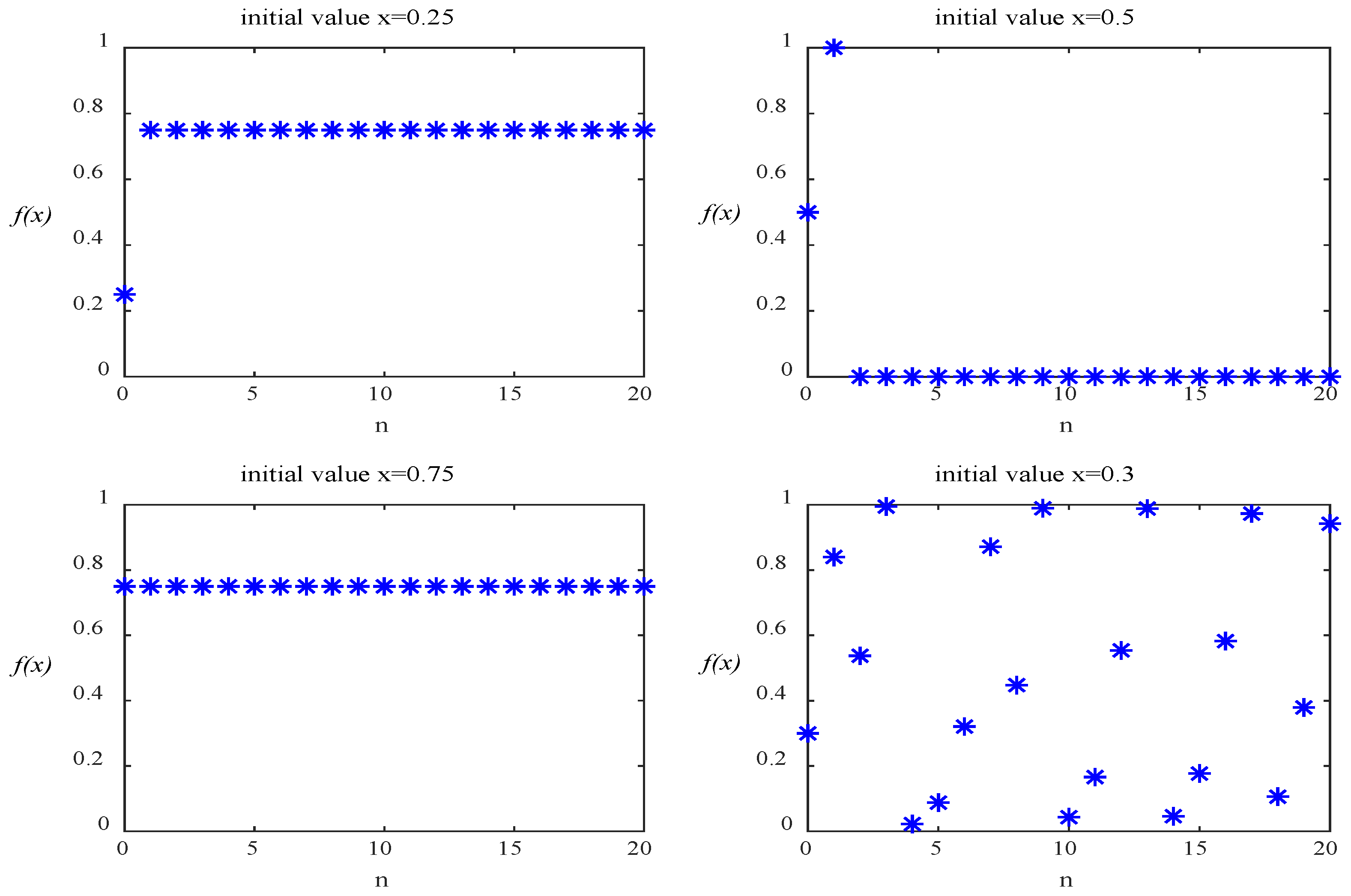
In the chaotic equation y = f x , x a , b , if there is an initial value x 0 a , b that makes f 0 = x 0 , then x 0 is called the fixed point of y . In logistic chaotic mapping, x 0 = 0.25 , 0.5   and   0.75 is a fixed point, and Figure 4 shows the properties of the fixed point. From Figure 4, it can be seen that when the initial value x 0 is a fixed point, the system loses ergodicity. x 0 0 , 1 , x 0 0.25 , 0.5 , 0.75 generates pseudo-random numbers x n 0 , 1 4 r after many iterations. When r = 4 , x n 0 , 1 is constant, and the system is in a completely chaotic state and has all the characteristics of a chaotic system. That is to say, the sequence generated by the initial condition x 0 = 0.3 is aperiodic and non-convergent.
Most of the initial populations of traditional genetic algorithms are completely randomly generated, while according to Darwin’s theory of evolution, most seemingly random species evolution in real biological systems follows certain rules—genetic theory. In order to better understand the advantages of chaos, this paper compares and analyzes chaotic phenomena and random phenomena. Although chaos and randomness appear to be unpredictable on the surface, the unpredictability of chaos is due to the lack of existing technology, which makes it difficult to overcome problems such as computing power or data collection. Long-term accurate prediction cannot be carried out, etc.; and the unpredictability of random phenomena is its essential property, which is congenital. In this paper, the internal randomness of chaos is used to ensure the diversity of initial solutions in genetic algorithm.
The steps for generating the initial population are as follows:
(1)
Setting parameters: population size is p o p _ s i z e , chromosome length is n , logistic chaotic mapping coefficient is r .
(2)
The initial values of p o p _ s i z e logistic chaotic maps are randomly generated.
(3)
The chaotic system of p o p _ s i z e groups (each group consists of n values) is calculated by Equation (20).
(4)
The initial population is generated according to the positions of n values in the chaotic system within their respective groups.
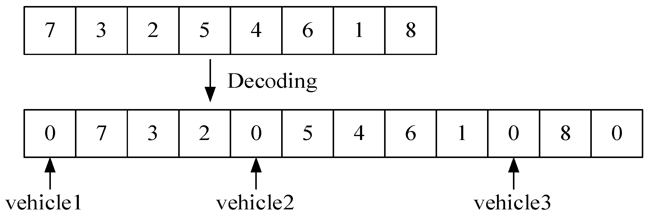
After the initial population is generated based on the logistic chaotic map, the nearest neighbor method is used to decode. Customers are divided into vehicles according to the initial sequence through vehicle load constraint and duration constraint tests. When the vehicle cannot meet the constraint, send a new vehicle to visit the customer and insert 0 before the customer who cannot meet the constraint, and so on until the last customer, and insert 0 at the beginning and end of the chromosome to complete decoding. As shown in Figure 5, assuming that the order of customers is 7-3-2-5-4-6-1-8, the first vehicle is dispatched to visit according to the order of customers. If the vehicle cannot meet the constraint when visiting customer 5, it will dispatch a new vehicle to visit customer 5, insert 0 in front of customer 5, and so on until customer 8 is visited, and insert 0 in front of customer 7 and after customer 8 to complete decoding. Finally, three routes are formed, i.e., vehicle1: 0-7-3-2-0; vehicle2: 0-5-4-6-1-0; vehicle3: 0-8-0.

3.2. Fitness Function

The fitness function can be calculated as follows:
f R = 1 C R
where C R represents the objective function.

3.3. Select Operation

The selection operation combines the elite reservations with the roulette wheel selection. First, the roulette wheel selection is to calculate the selected probability. Secondly, individual A with the highest probability is stored in the temporary matrix. After completing the search, if there is no better solution, it calculates the similarity between individual A and the sub-generation individuals. Next, it replaces the individual with the highest similarity.

3.4. Evolutionary Operation

In accordance with Figure 6, it selects two parents from individuals randomly. Firstly, points i 11 , i 12 , i 21 and i 22 are randomly generated, respectively, the part between i 11 and i 12 of the parent A is taken as the first segment of the sub-generation A 1 and the subsequent points of the sub-generation A 1 are related to the parent B , i.e., the customer points between i 11 and i 12 in the parent B are eliminated first. In the elimination process, the position sequence of the customer points in the parent B is not changed, and then the eliminated customer points are arranged as the second segment of the sub-generation A 1 to form the sub-generation A 1 and the sub-generation B 1 .

3.5. Local Search Strategy

Local search strategy is the core function of the algorithm, which determines the local search capability of the algorithm. In this paper, we adopt VNS algorithm applied to the local search strategy to strengthen the search capability.

3.5.1. Neighborhood Structure

(1)
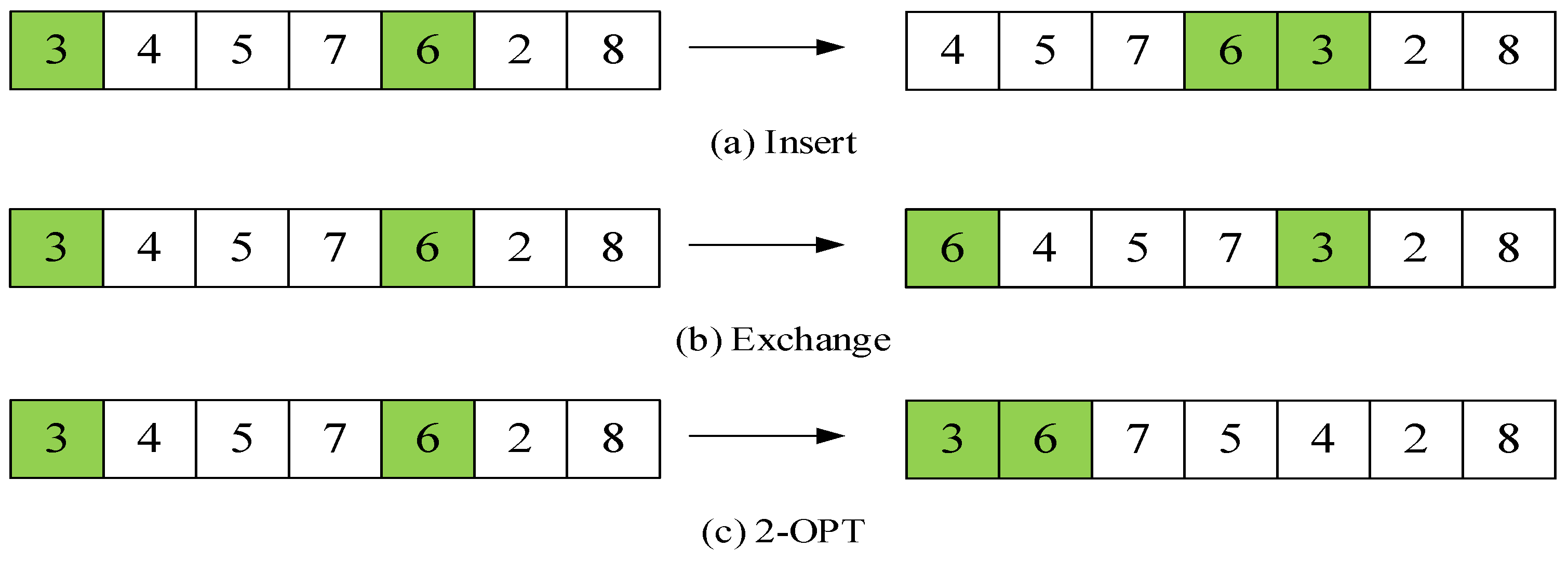
Insert: Randomly select customers i and j , and insert customer i after customer j . As shown in Figure 7a, customer 3 is inserted after customer 6.
(2)
Exchange: Randomly select customers i and j , then their positions are exchanged. As shown in Figure 7b, customer 3 and customer 6 are exchanged their locations.
(3)
2-OPT: Randomly select customers i and j , and the order of other customers among them are exchanged. As shown in Figure 7c, the position of customer 3 is kept unchanged, and customers 4, 5, 7, and 6 are in reverse order.

3.5.2. Adaptive Mechanism and Solution Acceptance

We design an adaptive neighborhood search number strategy and a new solution acceptance rule to balance the breadth and depth required for evolution, so that the algorithm jumps out of the local optimum. The disturbance intensity required by the population is different at different stages of the algorithm iteration. The strategy of adaptive neighborhood search times in this paper is as follows:
S n = τ 1 + τ 2 g e n M A X G E N
In Equation (22), S n is the number of search times, τ 1 is the minimum number of searches, τ 2 is the adaptive number of searches, ⎣ ⎦ represents round down, g e n is the current iteration number, M A X G E N is the maximum iteration number. It can be seen from Equation (22) that as the iteration number increases, the search times and depth gradually increase.
Equation (23) is the probability of new solution acceptance. x is a new solution.
p = 1 ,   C x C x exp C x C x , g e n , C x < C x ,

4. Instance Verification and Result Analysis

4.1. Algorithm Test

At present, there is no benchmark instance of TDGVRPFDTW. This paper selects instances of VRPTW and VRPFD to test the algorithm. The algorithm is programmed with MATLAB2018b in the Windows10 system. The proper setting of parameters has a great influence on the performance of heuristic algorithm. We analyze the function of parameters first. Next, we analyze the influence of parameters on solutions. Finally, we set the parameters through experiments. Setting the population size p o p _ s i z e and the maximum iteration number M A X G E N increases with the increase of the number of customers, and setting the adaptive parameters τ 1 = 1 , τ 2 = M A X G E N / 8 , and the local search repetition number max _ N = 50 of each generation.

4.1.1. Instance Analysis of VRPTW

In this paper, the R1 set in Solomon benchmark instances is selected (instance source: http://w.cba.neu.edu/~msolomon/problems.htm, accessed on 2 August 2022). Some have very tight time windows, while others have time windows that are hardly constraining. Set c 2 = 150 , c 3 = c 4 = 1 , the transportation cost between two nodes is l i j . Table 1 shows the best-known solution under hard time constraints and the operation results of the wasp colony algorithm (WCA) [35] and CGA_VNS under soft time window constraints. N is the number of vehicles, Trans_cost is the transportation cost, P_cost is the time window penalty costs, Total_cost is the total costs, Gap is the deviation between the optimal solution obtained by CGA_VNS and WCA, and Ave_gap is the average value of Gap.
The time complexity of CGA_VNS is O M A X G E N M a x _ N S n P o p _ s i z e N . It takes about 2.5 min to solve the R1. Table 1 shows that in the results of the 10 benchmark instances, the minimum G a p is −21.38%, the maximum G a p is 5.48%, and Ave_gap is −5.96%. Although the number of vehicles used in the results of R107, R108, and R108 optimized by CGA_VNS is more than that optimized by WCA, the time window penalty cost is greatly reduced, and the total cost is smaller. The effectiveness of CGA_VNS in solving VRPSTW can be verified by comparing the results.

4.1.2. Instance Analysis of VRPFD

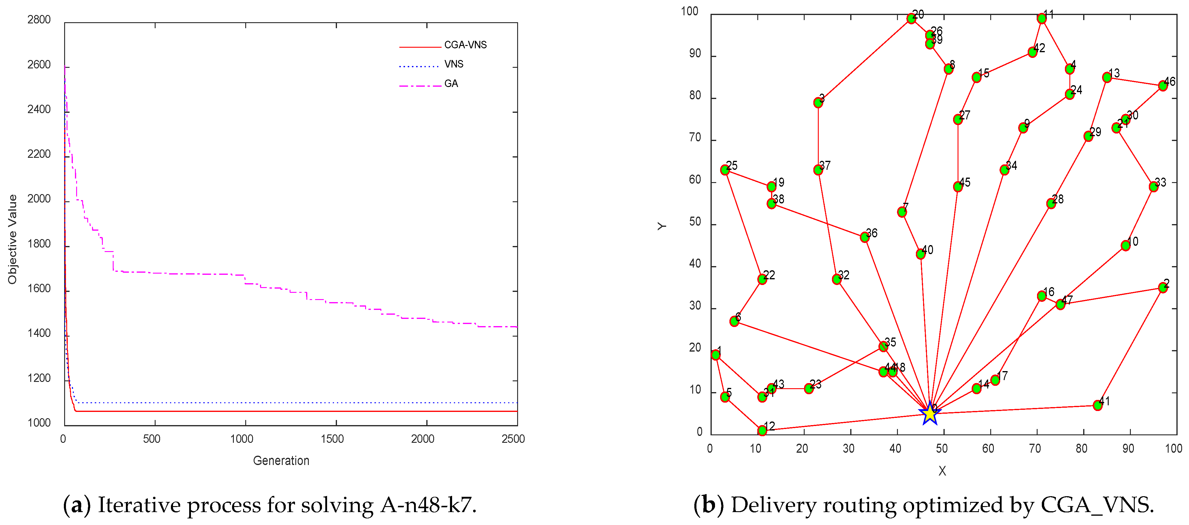
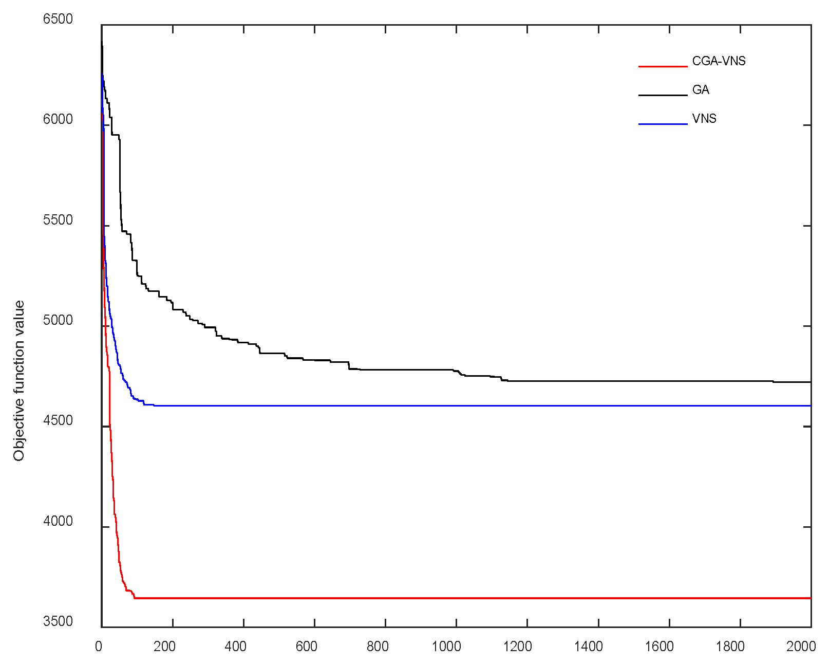
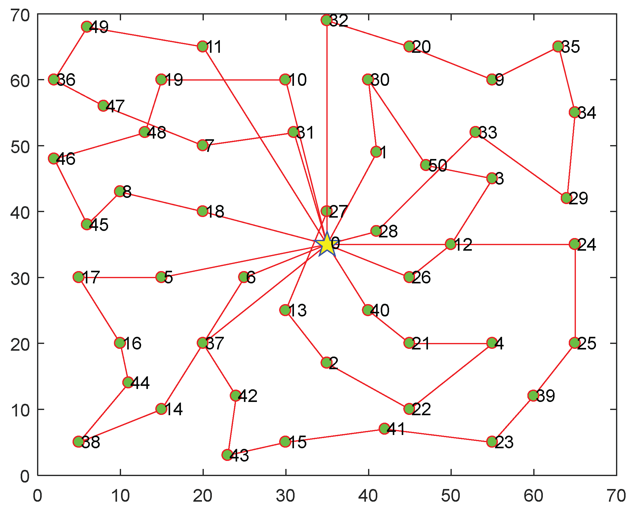
VRPFD is the basic problem of this paper. To test the performance of CGA_VNS to solve VRPFD, improve the A part of the reference [36] to form a test set. Let d ~ = 0.75 d , d , 1.25 d , the actual customer demand is d . Table 2 shows the pre-optimization results of GA, VNS, and CGA_VNS under different preference values, and t is the average time spent by the algorithm. Figure 8 shows the iterative process of solving A-n48-k7 by three algorithms and the optimal routing of CGA_VNS optimization when the decision preference value is 0.4. It can be seen from Table 2 and Figure 8a that the convergence speed of GA is slow, the time spent in one experiment is relatively long, and the solution quality is poor. Compared with VNS, CGA_VNS adds an order crossover operator. Although CGA_VNS takes a little longer time to run once than VNS, it increases its local search ability and has better solution quality, and obtains the best solution of all instances under different decision preference values. Therefore, CGA_VNS has better performance than GA and VNS.
In this paper, Zhang et al. [5] improved A-n32-k5 is selected to further verify the performance of the algorithm, The optimal solutions of variable neighborhood scatter search algorithm (VNSS) [5], variable neighborhood tabu search algorithm (VNTS) [6] and the CGA_VNS running 10 times are summarized in Table 3. N represents the number of vehicles used in the pre-optimization scheme, Best represents the best value of the pre-optimization scheme, Ave is the average of the results of 10 operations and Gap is the deviation between the best solution obtained by CGA_VNS and the best-known solution. t is the time spent in one experiment. It can be seen from Table 3 that the results obtained by CGA_VNS are not inferior to VNSS and VNTS except that is 0.1, and the results obtained by CGA_VNS are relatively stable. The performance of the algorithm is further verified.

4.2. Numerical Experiment

At present, there are no benchmark instances of the TDGVRPTWFD. This paper improves the data of the top 50 customers of R101 in the Solomon database as the instance in this paper. The parameters are set as follows: d = 0.25 d / 25 , d / 25 , 1.25 d / 25 , the customer’s time window is E T / 20 + 0.5 , L T / 20 + 0.5 , Q = 5 t , c 1 = 6.9 , c 2 = 500 , c 3 = 2 , c 4 = 3 , T 0 d = 6 : 00 , t i k = 0.5 . We consider three types of roads, urban main roads, secondary roads, and branch roads. In Figure 9, red and black represent main roads and secondary roads respectively. Undrawn routes are branch roads. Figure 10 is vehicle speeds.

4.2.1. Pre-Optimization Stage

To verify the performance of CGA_VNS to solve the problems in this paper, GA, VNS, and CGA_VNS were used to solve the instance in the pre-optimization stage and the results were compared. Table 4 shows the pre-optimization results of the algorithm under different preference values, B e s t / N represents the optimal value of the solution and the number of vehicles used, W o r s t / N represents the worst value of the solution and the number of vehicles used, A v e represents the average value of the solution results, and S D is the standard deviation of the solution results. Figure 11 shows the convergence process of the algorithm when α = 0 . 4 . Figure 12 is a pre-optimized delivery route solved by CGA_VNS when α = 0 . 8 .
It can be seen from Table 4: (1) CGA_VNS obtains the pre-optimized optimal solution under all preference values and the standard deviation of the result is the smallest, which shows that CGA_VNS has higher solution quality and better solution stability than the other two algorithms. It can be seen from Figure 11 that CGA_VNS has a faster convergence speed. (2) Decision-makers’ preference value has a great influence on distribution costs. The costs of the pre-optimization solution increase with the increase of α , and the number of vehicles dispatched also increases, gradually increasing from 4 vehicles with α 0.1 , 0.2 to 8 vehicles with α = 1 .

4.2.2. Re-Optimization Stage

Assuming that the actual demand of the served customers is d 1 = d / 25 , Table 5 shows the re-optimization results corresponding to the best pre-optimization results under different preference values. Strategy 1 is the failure node return strategy, strategy 2 is the pre-failure node return strategy, and strategy 3 is the optimization strategy in this paper. P r e b e s t is the best pre-optimization result, E cos t is the extra costs of the pre-optimization scheme due to route failure, T cos t is the total distribution costs after re-optimization, Re b e s t is the lowest total costs of the three strategies. Table 5 shows that when α 0.1 , 0.4 the pre-optimization scheme needs to be re-optimized, the extra costs of the distribution scheme solved by the strategy in this paper are lower than the other two strategies. Table 6 gives detailed adjustment results when α = 0.4 .
Based on the above analysis, the essence of the three strategies is to maintain a certain degree of balance between risk and costs. The strategy in this paper is better than strategy 1 and strategy 2 on the whole.

5. Conclusions

In reality, due to the existence of objective and subjective factors, customer demand is often fuzzy and uncertain. Meanwhile, the dynamic change of traffic information will also affect the formulation of the distribution scheme. For TDGVRPTWFD, this paper comprehensively considers the influence of the dispatch costs, fuel costs, and time window penalty costs on the total costs, and establishes a fuzzy chance-constrained optimization model with time-varying vehicle speed and time window. In the pre-optimization stage, a pre-optimization scheme is generated based on the credibility measure theory. in the re-optimization stage, route adjustments will be made for customers who have failed in service. The chaotic genetic algorithm with variable neighborhood search is developed to solve the problem. Numerical results show that the model and algorithm are effective. The following conclusions are obtained:
(1)
The fuzzy chance-constrained optimization model of TDGVRPTWFD has fully considered the fuzziness of customer demand in the actual distribution process, further expanding and deepening the VRP research.
(2)
The model considers the time-dependent vehicle speed and the influence of vehicle speed, load, and road gradient on fuel consumption. After considering the above factors, the model becomes more complex and closer to the actual situation.
(3)
The proposed algorithm uses logistic chaotic mapping to generate initial solutions, which ensures the diversity of initial solutions. Adaptive neighborhood search times strategy and inferior solution acceptance mechanism improve the performance of algorithm.
(4)
In the pre-optimization stage, the distribution costs of the pre-optimization scheme increase with the increase of the preference value of decision-makers, and the number of vehicles dispatched also increases. In the re-optimization stage, the more conservative the decision-makers tend to be, the lower the extra costs they pay and the smaller the number of vehicles they dispatch.
The research in this paper takes into account the fuzziness of customer demand and the dynamic changes in the traffic environment, which is more in line with the actual distribution situation. The research results not only further enrich the research on VRP-related theories, but also provide a scientific basis for the distribution optimization decision-making of logistics enterprises.

Author Contributions

H.F. (Hao Fan) and X.R. provided the core idea of this paper, collected and analyzed the data. Y.Z. and Z.Z. wrote the manuscript. H.F. (Houming Fan) contributed to the conceptualization of this paper, and the provision of valuable comments. All authors have read and agreed to the published version of the manuscript.

Funding

This work was supported by the Special Project of National Emergency Management System Construction of Chinese National Funding of Social Science, Grant number 20VYJ024.

Institutional Review Board Statement

Not applicable.

Informed Consent Statement

Not applicable.

Data Availability Statement

Not applicable.

Conflicts of Interest

The authors declare no conflict of interest.

References

  1. Cao, E.; Lai, M. The open vehicle routing problem with fuzzy demands. Expert Syst. Appl. 2010, 37, 2405–2411. [Google Scholar] [CrossRef]
  2. Kuo, R.J.; Zulvia, F.E.; Suryadi, K. Hybrid particle swarm optimization with genetic algorithm for solving capacitated vehicle routing problem with fuzzy demand-A case study on garbage collection system. Appl. Math. Comput. 2012, 219, 2574–2588. [Google Scholar] [CrossRef]
  3. Wang, J.; Li, B. Dynamic management of vehicle routing problem with time windows and fuzzy demands based on the multi-objective optimization. Chinese J. Manag. 2013, 10, 238–243. [Google Scholar]
  4. Liu, C.S.; Kou, G.; Huang, F.H. Vehicle coordinated strategy for vehicle routing problem with fuzzy demands. Math. Probl. Eng. 2016, 9, 9071394. [Google Scholar] [CrossRef] [Green Version]
  5. Zhang, X.N.; Fan, H.M. Optimization and real-time adjustment for vehicle routing problem with fuzzy demand. Shanghai Jiaotong Univer. 2016, 50, 123–130. [Google Scholar]
  6. Li, Y.; Fan, H.M.; Zhang, X.; Yang, X. Two-stage variable neighborhood tabu search for the capacitated vehicle routing problem with fuzzy demand. Syst. Eng. Theory Pract. 2018, 38, 522–531. [Google Scholar]
  7. Giallanza, A.; Li Puma, G. Fuzzy green vehicle routing problem for designing a three echelons supply chain. J. Clean Prod. 2020, 259, 120774. [Google Scholar] [CrossRef]
  8. Fan, H.; Li, D.; Kong, L.; Ren, X. Optimization for time dependent vehicle routing problem with fuzzy demand and time windows. Con. Theory Appl. 2020, 37, 950–960. [Google Scholar]
  9. Hashimoto, H.; Yagiura, M.; Imahori, S.; Ibaraki, T. Recent progress of local search in handling the time window constraints of the vehicle routing problem. Ann. Oper. Res. 2010, 8, 221–238. [Google Scholar] [CrossRef]
  10. Yu, Y.; Wang, S.H.; Wang, J.W.; Huang, M. A branch-and-price algorithm for the heterogeneous fleet green vehicle routing problem with time windows. Transp. Res. Pt. B Methodol. 2019, 122, 511–527. [Google Scholar] [CrossRef]
  11. Wang, Y.; Wang, L.; Chen, G.C.; Cai, Z.Q.; Zhou, Y.Q.; Xing, L.N. An improved ant colony optimization algorithm to the periodic vehicle routing problem with time window and service choice. Swarm Evol. Comput. 2020, 55, 100675. [Google Scholar] [CrossRef]
  12. Marinakis, Y.; Marinaki, M.; Migdalas, A. A multi-adaptive particle swarm optimization for the vehicle routing problem with time windows. Inf. Sci. 2019, 481, 311–329. [Google Scholar] [CrossRef]
  13. Perez-Rodríguez, R.; Hernandez-Aguirre, A. A hybrid estimation of distribution algorithm for the vehicle routing problem with time windows. Comput. Ind. Eng. 2019, 130, 75–96. [Google Scholar] [CrossRef]
  14. Taniguchi, E.; Shimamoto, H. Intelligent transportation system based dynamic vehicle routing and scheduling with variable travel times. Transp. Res. Pt. C-Emerg. Technol. 2014, 12, 235–250. [Google Scholar] [CrossRef]
  15. Mancini, S. Time dependent travel speed vehicle routing and scheduling on a real road network: The case of Torino. Transp. Res. Procedia 2014, 3, 433–441. [Google Scholar] [CrossRef]
  16. Haghani, A.; Jung, S. A dynamic vehicle routing problem with time-dependent travel times. Comput. Oper. Res. 2005, 32, 2959–2986. [Google Scholar] [CrossRef]
  17. Hashimoto, H.; Yagiura, M.; Ibaraki, T. An iterated local search algorithm for the time-dependent vehicle routing problem with time windows. Discret. Optim. 2008, 5, 434–456. [Google Scholar] [CrossRef] [Green Version]
  18. Hu, C.; Lu, J.; Liu, X.; Zhang, G. Robust vehicle routing problem with hard time windows under demand and travel time uncertainty. Comput. Oper. Res. 2018, 94, 139–153. [Google Scholar] [CrossRef]
  19. Figliozzi, M.A. The time dependent vehicle routing problem with time windows: Benchmark problems, an efficient solution algorithm, and solution characteristics. Transp. Res. Pt. E-Logist. Transp. Rev. 2012, 48, 616–636. [Google Scholar] [CrossRef]
  20. Mu, D.; Wang, C.; Wang, S.C.; Zhou, S.C. Solving TDVRP based on parallel-simulated annealing algorithm. Comput. Int. Manuf. Syst. 2015, 21, 1626–1636. [Google Scholar]
  21. Kuo, Y.Y. Using simulated annealing to minimize fuel consumption for the time-dependent vehicle routing problem. Comput. Ind. Eng. 2010, 59, 157–165. [Google Scholar] [CrossRef]
  22. Liu, C.S.; Kou, G.; Zhou, X.C.; Peng, Y.; Sheng, H.F.; Alsaadi, F.E. Time-dependent vehicle routing problem with time windows of city logistics with a congestion avoidance approach. Knowl.-Based Syst. 2020, 188, 104813. [Google Scholar] [CrossRef]
  23. Poonthalir, G.; Nadarajan, R. A fuel efficient green vehicle routing problem with varying speed constraint (F-GVRP). Expert Syst. Appl. 2018, 100, 131–144. [Google Scholar] [CrossRef]
  24. Xu, Z.; Elomri, A.; Pokharel, S.; Mutlu, F. A model for capacitated green vehicle routing problem with the time varying vehicle speed and soft time windows. Comput. Ind. Eng. 2019, 137, 106011. [Google Scholar] [CrossRef]
  25. Xiao, Y.; Konak, A. The heterogeneous green vehicle routing and scheduling problem with time-varying traffic congestion. Transp. Res. Pt. E-Logist. Transp. Rev. 2016, 88, 146–166. [Google Scholar] [CrossRef]
  26. Çimen, M.; Soysal, M. Time-dependent green vehicle routing problem with stochastic vehicle speeds: An approximate dynamic programming algorithm. Transp. Res. Part D-Transp. Environ. 2017, 54, 82–98. [Google Scholar] [CrossRef]
  27. Yang, H. Research of Urban Recurrent Congestion Evolution based on Taxi GPS Date. Doctoral Thesis, Harbin Institute of Technology, Harbin, China, 2018. [Google Scholar]
  28. Hickman, J.; Hassel, D.; Joumard, R.; Samaras, Z.; Sorenson, S. MEET Methodology for Calculating Transport Emissions and Energy Consumption; Technical Report DG VII; European Commission: Brussels, Belgium, 1999. [Google Scholar]
  29. Alinaghian, M.; Naderipour, M. A novel comprehensive macroscopic model for time-dependent vehicle routing problem with multi-alternative graph to reduce fuel consumption: A case study. Comput. Ind. Eng. 2016, 99, 210–222. [Google Scholar] [CrossRef]
  30. Cao, E.B.; Lai, M.Y. A hybrid differential evolution algorithm to vehicle routing problem with fuzzy demands. J. Comput. Appl. Math. 2009, 231, 302–310. [Google Scholar]
  31. Yang, W.; Mathur, K.; Ballou, R.H. Stochastic vehicle routing problem with restocking. Transp. Sci. 2000, 34, 99–112. [Google Scholar] [CrossRef]
  32. Xie, B.L.; An, S.; Guo, Y.H. Multi-tour optimization policy for stochastic vehicle routing problem. Syst. Eng. Theory Prac. 2007, 27, 167–171. [Google Scholar]
  33. Zhao, Y.; Li, C.; Zhang, J.; Lu, Y.; Wang, W. Novel algorithm for multi-objective vehicle routing problem with stochastic demand. Comput. Integr. Manuf. Syst. 2012, 18, 523–530. [Google Scholar]
  34. Fan, H.M.; Liu, P.C.; Liu, H.; Hou, D.K. The multi-depot vehicle routing problem with simultaneous deterministic delivery and stochastic pickup based on joint distribution. Acta Auto Sinica 2021, 47, 1–15. [Google Scholar]
  35. Yang, J.; Ma, L. Wasp Colony Algorithm for Vehicle Routing Problem with Soft Time Windows. Appl. Res. Comput. 2010, 29, 67–70+61. [Google Scholar]
  36. Augerat, P.; Belenguer, J.M.; Benavent, E.; Corberan, A.; Rinaldi, G. Computational Results with a Branch and Cut Code for the Capacitated Vehicle Routing Problem; Rapport de Recherche-IMAG; Universite Joseph Fourier: Grenoble, France, 1998; p. 495. [Google Scholar]
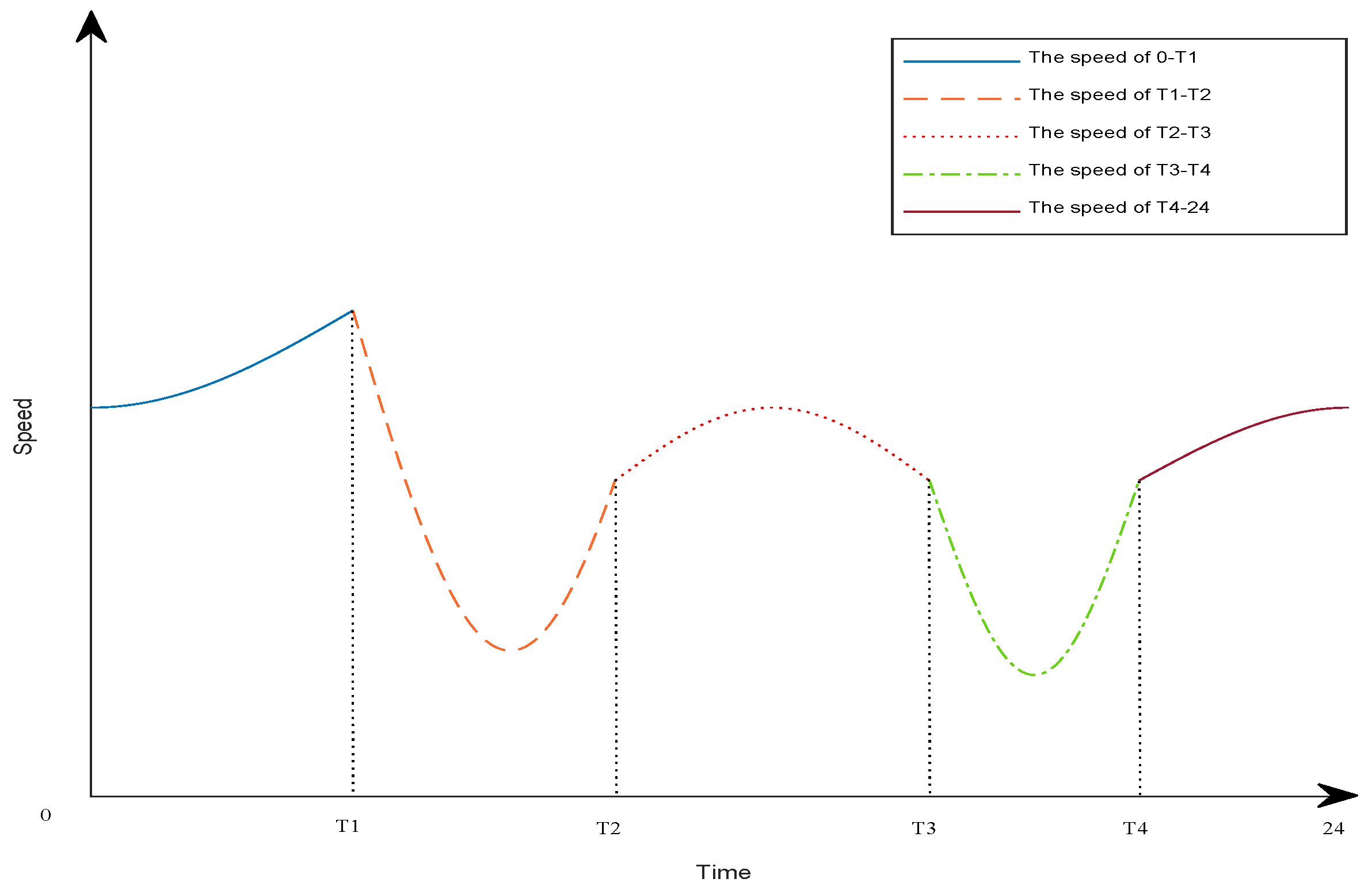
Figure 1. Variation trend of vehicle speed.
Symmetry 14 02115 g001
Figure 2. Different failure node re-optimized strategies.
Symmetry 14 02115 g002
Figure 3. The basic flow of CGA_VNS.
Symmetry 14 02115 g003
Figure 4. Logistic chaotic mapping fixed point.
Symmetry 14 02115 g004
Figure 5. Decoding diagram.
Symmetry 14 02115 g005
Figure 6. The diagram of the order crossover operator.
Symmetry 14 02115 g006
Figure 7. Neighborhood structures.
Symmetry 14 02115 g007
Figure 8. Iterative process and delivery path for solving A-n48-k7 (α = 0.4).
Symmetry 14 02115 g008
Figure 9. Distribution road network.
Symmetry 14 02115 g009
Figure 10. The time-dependent function of speed.
Symmetry 14 02115 g010
Figure 11. Convergence process diagram ( α = 0.4 ).
Symmetry 14 02115 g011
Figure 12. Pre-optimized routing ( α = 0.8 ).
Symmetry 14 02115 g012
Table 1. Comparison of CGA_VNS with other heuristics on VRPSTW instances.
InstanceVRPHTWWCACGA_VNSGap
NDNTrans_costP_costTotal_costNTrans_costP_costTotal_cost
R101191645.79121564.49721.204085.69111347.891226.884224.773.40%
R102171486.12111376.37760.003786.37111336.07841.293827.361.08%
R103131292.6891141.141173.763664.9101163.59417.573081.16−15.93%
R10491007.2481017.82811.533029.359936.02476.412762.43−8.81%
R105141377.11101228.631055.703784.33101172.321113.583785.90.04%
R106121251.9891127.401395.043872.4491041.131116.563507.69−9.42%
R107101104.6681066.831451.953718.7891015.70557.932923.63−21.38%
R1089960.888986.88760.242947.129946.00198.182494.18−15.37%
R109111194.7391137.75908.403396.15101152.49786.243438.731.25%
R110101118.5991100.66553.293003.9591091.81726.843168.655.48%
Ave_gap−5.96%
WCA runs with Microsoft Visual Studio 2005 in Windows XP, and the time complexity is o m n 2 .
Table 2. Comparison of CGA_VNS with GA and VNS.
α0.10.20.30.40.50.60.70.80.91t/s
Instance
& Algorithm
A-n36-k5CGA_VNS7117247687708028188518779029027.3
VNS7127247797708118318668999029066.2
GA803835845882879945944965974100718.21
A-n44-k7CGA_VNS852872898933939965101010311063109312.0
VNS86487290494494997810301035106911089.5
GA99510791040110111311200114011841148122420.9
A-n48-k7CGA_VNS9429771038106411111115117912211240126714.1
VNS9599961040107511091142122412381243130911.4
GA119412121264125812981301138714011407149025.8
A-n55-k9CGA_VNS9519921012106110821122116311781233128220.7
VNS95710151025106811221157117512371246127917.1
GA122212951312128313311340133714331446149035.4
A-n65-k9CGA_VNS106910921121118612111266129513531417143126.2
VNS109710961168122312591305129813731477148724.2
GA148415381508152516151671174116881745170663.8
A-n69-k9CGA_VNS106411061138118511951247128613131333138026.8
VNS107211211149124112371310132113501375139025.6
GA125513211483147915821547155415741610168771.35
Table 3. Results of comparison between CGA_VNS and VNSS, VNTS.
αVNSSVNTSCGA_VNSt/sGap
NBestAveNBestAveNBestAve
0.14686686468668646876874.30.14%
0.24719719471971947197194.30
0.34727727472772747277274.20
0.45755755.7575575547557554.50
0.55784784578478457847844.30
0.65796796579679657967964.20
0.7584884858488485848851.14.20
0.85880883.3586886858688684.50
0.95882887.658828825882882.84.30
1.06892892.268928926892893.34.40
Table 4. Pre-optimization results under different preference values.
αGAVNSCGA_VNS
Best/NWorst/NAveSDBest/NWorst/NAveSDBest/NWorst/NAveSD
0.14170.9/54198.0/54188.3123995.0/54090.0/54045.6393092.4/43120.4/43109.712
0.24011.1/54117.1/54066.7433992.5/54025.5/54013.3153067.4/43106.5/43091.717
0.33968.8/54320.8/541281463981.4/54038.3/54010.7233622.0/53650.8/5364013
0.44700.8/64723.5/6471393965.1/54604.3/64188.42943644.8/53697.3/53673.922
0.54547.7/64599.2/64566.3234472.0/64517.4/64491.6194249.5/64311.4/64272.528
0.65025.6/75117.9/75073.8384994.4/75042.8/75013.7214797.3/74820.0/74807.29
0.75030.9/75058.0/75045.7114891.8/75021.8/74953.6534779.7/74863.1/74811.837
0.85067.0/75149.3/75108345034.2/75175.3/75097.1594832.3/74866.3/74848.814
0.95265.3/75455.7/75321.91205338.9/75605.3/85522.61304912.7/74958.3/74936.719
15654.5/85720.0/85702.1345556.6/85642.0/85591.5375402.1/85426.3/85409.312
Ave 47 69 18
Table 5. Results of different re-optimization strategies.
αPre-BestStrategy 1Strategy 2Strategy 3Re-Best
E-CostT-CostE-CostT-CostE-CostT-Cost
0.13092.4536.83629.2466.33558.7327.33419.73419.7
0.23067.4514.63582.0460.13527.5343.63411.03411.0
0.33622.0544.64166.6496.84118.8376.73998.73998.7
0.43644.8594.54239.3533.14177.9276.03920.83920.8
0.54249.504249.504249.504249.54249.5
0.64797.304797.304797.304797.34797.3
0.74779.704779.704779.704779.74779.7
0.84832.304832.304832.304832.34832.3
0.94912.704912.704912.704912.74912.7
15402.105402.105402.105402.15402.1
Table 6. Re-optimization result when α = 0.4 .
Pre-Optimization SchemeStrategy 1Strategy 2Strategy 3
V1: 0-27-31-7-11-32-33-3-29-24-25-26-0;V1: 0-27-31-7-11-32-33-3-29-24-25-0-25-26-0;V1: 0-27-31-7-11-32-33-3-29-24-0-25-26-0;V1: 0-27-31-7-11-32-33-3-29-24-0;
V2: 0-28-12-4-39-23-22-21-0;V2: 0-28-12-4-39-23-22-0-22-21-0;V2: 0-28-12-4-39-23-0-22-21-0;V2: 0-28-12-4-39-23-0;
V3: 0-18-8-47-36-49-19-20-9-35-34-0;V3: 0-18-8-47-36-49-19-20-9-35-0-35-34-0;V3: 0-18-8-47-36-49-19-20-9-0-35-34-0;V3: 0-18-8-47-36-49-19-20-9-0;
V4: 6-5-17-45-46-48-10-30-50-1-0;V4: 6-5-17-45-46-48-10-30-50-0-50-1-0;V4: 6-5-17-45-46-48-10-30-0-50-1-0;V4: 6-5-17-45-46-48-10-30-0;
V5: 0-40-2-41-15-43-42-14-44-38-16-37-13-0;V5: 0-40-2-41-15-43-42-14-44-38-16-37-13-0-13-0;V5: 0-40-2-41-15-43-42-14-44-38-16-37-0-13-0;V5: 0-40-2-41-15-43-42-14-44-38-16-37-0;
V1′: 0-25-13-22-21-26-0;
V2′: 0-34-25-1-50;
Publisher’s Note: MDPI stays neutral with regard to jurisdictional claims in published maps and institutional affiliations.