Analytical Model with Independent Control of Load–Displacement Curve Branches for Brittle Material Strength Prediction Using Pre-Peak Test Loads

Abstract

The relevance of problems related to the fracturing of engineering materials and structures will not decrease over time. Fracture mechanics methods continue to be developed, which, combined with numerical methods of computer modeling, are implemented in software packages. However, this is only one facet of the complex of actual problems related to modeling and analyzing the behavior of brittle materials. No less important are the problems of developing not only numerical, but also new analytical models. In this paper, analytical models of only one class are considered, the distinguishing feature of which is that they describe the full load–strain curve using only one equation. However, the determination of model parameters requires tests for which the destruction of the test object is necessary, which may be unacceptable if controlled destruction is technically impossible or economically unreasonable. At the same time, in practice, it is possible to obtain values of stresses and strains caused by loads smaller than the peak load. Pre-peak loads can be used to predict strength using numerical methods, but it is desirable to have a suitable analytical model to extend the capabilities and to reduce the cost of applied research. Such a model was not found in the known literature, which motivated this work, which aims to modify the analytical model to predict strength and the full load–displacement (or stress–strain) curve using only pre-peak loading. This study is based on the analysis of known data and synthesis using mathematical modeling and fracture mechanics. The input data for the model do not include the particle size distribution and other physical and mechanical properties of the components of the material under study. These properties may remain unknown, but their influence is taken into account indirectly according to the “black box” methodology. Restrictions of the scope of the model are defined. The simulation results are consistent with experiments known from the literature.

1. Introduction

1.1. General Description of the Research Problem

The problems of the damage and destruction of engineering materials and structures, due to the objective necessity accompanying the development of civilization, have remained topical for many years. Damage and fracture analysis has gradually become an independent branch of materials and structures mechanics [1,2,3]. Methods of fracture mechanics combined with numerical methods of computer modeling are implemented in software complexes, which are effective tools to analyze and predict the mechanical state of engineering structures and their fragments [4,5,6,7,8]. However, this is only one facet of the complex of actual problems of modeling and analyzing the behavior of materials in the brittle state. Equally important are the problems of transition from discrete to continuous behavior as well as the evaluation of the significance and calibration of model parameters, which involves the development of not only numerical but also new analytical models of fracture mechanics [9].

1.2. Existing Models of the Class in Question and the Purpose of the Study

This work aimed at modeling brittle materials, such as concrete, rocks, frozen ground, and some new polymers [10]. Many models of brittle materials are known from the literature [11,12,13,14]. Commenting on this is beyond the scope of this article, in which the focus is on models of only one class, an overview of which can be found in the article [15]. There are few such models yet, but they are very promising. A distinctive feature of models of this class is that they describe the complete load–strain curve with only one equation for a very small amount of input data. The first model of this class, known as the Furamura model, was used to analyze the temperature behavior of concrete [16]. Stojković et al. (2017) analyzed the known models of this class and, based on them, proposed a new, more universal two-parameter model [15].

In the Furamura model noted above [15], the full stress–strain curve is described by Equation (1):

$$\sigma ={\sigma }_{peak}\frac{\epsilon }{{\epsilon }_{peak}}{e}^{\left(1-\frac{\epsilon }{{\epsilon }_{peak}}\right)}.$$

(1)

Here, ${\sigma }_{peak}$ and ${\epsilon }_{peak}$ are, respectively, the peak stress $\sigma$ and strain $\epsilon$.

Blagojevich [17] proposed a model that is a modified Expression (1) with an additional parameter $c$:

$$\sigma ={\sigma }_{peak}{\left(\frac{\epsilon }{{\epsilon }_{peak}}{e}^{\left(1-\frac{\epsilon }{{\epsilon }_{peak}}\right)}\right)}^c.$$

(2)

The parameter $c$ can be obtained by fitting the curve to experimental data. Figure 1 shows examples of curves σ = σ(ε) by Equation (2) for some values of parameter $c$ if ${\sigma }_{peak}=2.5$ MPa and ${\epsilon }_{peak}=0.02$.

If $c=1$ (red line in Figure 1), we obtain the Furamura model (1) as a special case of the Blagojevich model (2). Unlike model (1), in model (2), there appears an inflection point on left branch of full curve if $c>1$. Using Equation (2), coordinates ε of inflection points of left and right branches can be found from condition $d^2\sigma /d{\epsilon }^2=0$, respectively, $\epsilon =\left(\sqrt{c}-1\right)c^{-1/2}{\epsilon }_{peak}$ and $\epsilon =\left(\sqrt{c}+1\right)c^{-1/2}{\epsilon }_{peak}$.

Revealing the potential of model (2), Stojković et al. [15] proposed a model with interval parameter $\alpha \le c\le \beta$:

$$\sigma ={\sigma }_{peak}{\left(\frac{\epsilon }{{\epsilon }_{peak}}{e}^{\left(1-\frac{\epsilon }{{\epsilon }_{peak}}\right)}\right)}^{\left(\alpha -\frac{\epsilon }{{\epsilon }_{peak}}\left(\alpha -\beta \right)\right)}.$$

(3)

The parameters $\alpha$ and $\beta$ can be obtained by fitting to experimental data using the least squares method, as shown in [15]. In order to use models (1)–(3), the values of ${\sigma }_{peak}$ and ${\epsilon }_{peak}$ should be obtained from the experimental stress–strain curve [15]. However, the direct experimental determination of ${\sigma }_{peak}$ and ${\epsilon }_{peak}$ is usually accompanied by a failure of the structure or sample, which may be unacceptable if controlled failure is not technically possible or economically feasible. In practice, however, it is possible to obtain values of $\sigma <{\sigma }_{peak}$ and $\epsilon <{\epsilon }_{peak}$ for several points on the left branch of the stress–strain curve (Figure 1). These values could be used to predict ${\sigma }_{peak}$ and ${\epsilon }_{peak}$ values using numerical methods. However, in order to expand the possibilities of applied research, it is advisable to have an analytical model for predicting ${\sigma }_{peak}$ and ${\epsilon }_{peak}$ values; such a model could not be found in the known literature. Considering this circumstance, the working hypothesis of the presented study was formulated: based on previous studies, a modification of the model can be developed for the analytical prediction of ${\sigma }_{peak}$ and ${\epsilon }_{peak}$ values and the complete load–displacement (or stress–strain) curve using only the pre-peak test load. The development of the indicated model is the purpose of this paper.

1.3. A Flow Chart of the Research Approach

This study is based on the analysis of known data and synthesis using the ideas of mathematical modeling and fracture mechanics of brittle materials, reflected in the literature cited above [1,2,3,4,5,6,7,8,9,10,11,12,13,14,15,16,17]. The contributions of this study, taking into account the contents of Section 1.1 and Section 1.2, as well as methodological aspects, include:

• A brief review of the literature and justification of the problem, working hypothesis, and purpose of the study.
• A review of analytical models, the distinctive feature of which is that they describe the full load–strain curve for brittle materials using only one equation: methodological aspects.
• The development of a model with completely separate control of the left and right branches of the load–strain curve using the Heaviside function.
• The application of the model to the analysis of known data and comparison of simulation results with experimental data.
• The application of the developed model to predict the peak external load (bearing capacity) based on the results of pre-peak tests.
• The development of a prediction algorithm.
• An analysis of the limitations of the scope of the algorithm.
• An analysis of examples of applications of the developed model and methodology for forecasting peak values of external load for brittle materials.
• A discussion of the results and analysis of the possible development of the topic of the performed research to improve the understanding of the behavior of brittle materials during their loading, as well as concluding remarks.

2. Methodology

2.1. Preliminary Remarks

From a methodological point of view, model (3) is based on the idea of the decomposition of parameter $c$ (2); the implementation of this idea improved the universality of the model and the accuracy of the simulation results [15].

Based on the same idea of the decomposition of parameter $c$ in model (2), it is possible to develop another model with the independent control of the upstream and downstream branches of the stress–strain curve, but with a smooth node at the connection point of these branches (i.e., at the point with coordinates ${\sigma }_{peak}$ and ${\epsilon }_{peak}$ (Figure 1)). In this case, the question arises: Why is it reasonable to control the pre-peak and post-peak branches separately? Answering this question, we note the following physical aspects: The loading and deformation of a brittle material is accompanied by the growth of micro-, meso-, and macro-cracks. The weakest material particles collapse and fail. As a consequence, the bearing capacity of the sample (or structure) gradually decreases, which is modeled by the post-peak branch of the load–strain curve (Figure 1). The load is redistributed to those particles that are not yet destroyed, so the average stress in the material of these particles increases despite the load reduction [18]. In the process under consideration, the material properties of each particle remain unchanged if the mechanical load is not accompanied by a temperature effect, which affects the elastic modulus and other physical properties of the material.

Thus, a brittle material, as a mechanical system of meso-particles, continuously degrades if the load increases, and therefore the characteristics of this system in the pre-peak state will differ markedly from those in the post-peak state. Accordingly, each of the two branches of the load–strain curve should reflect these changes; the curve equation should contain two parameters. Such parameters in model (3) are $\alpha$ and $\beta$, which, however, remain interdependent in the general case. Therefore, model (3) can be classified as a model with limited pre- and post-peak branch control. A model with the completely separate control of the right and left branches is proposed in the following subsection.

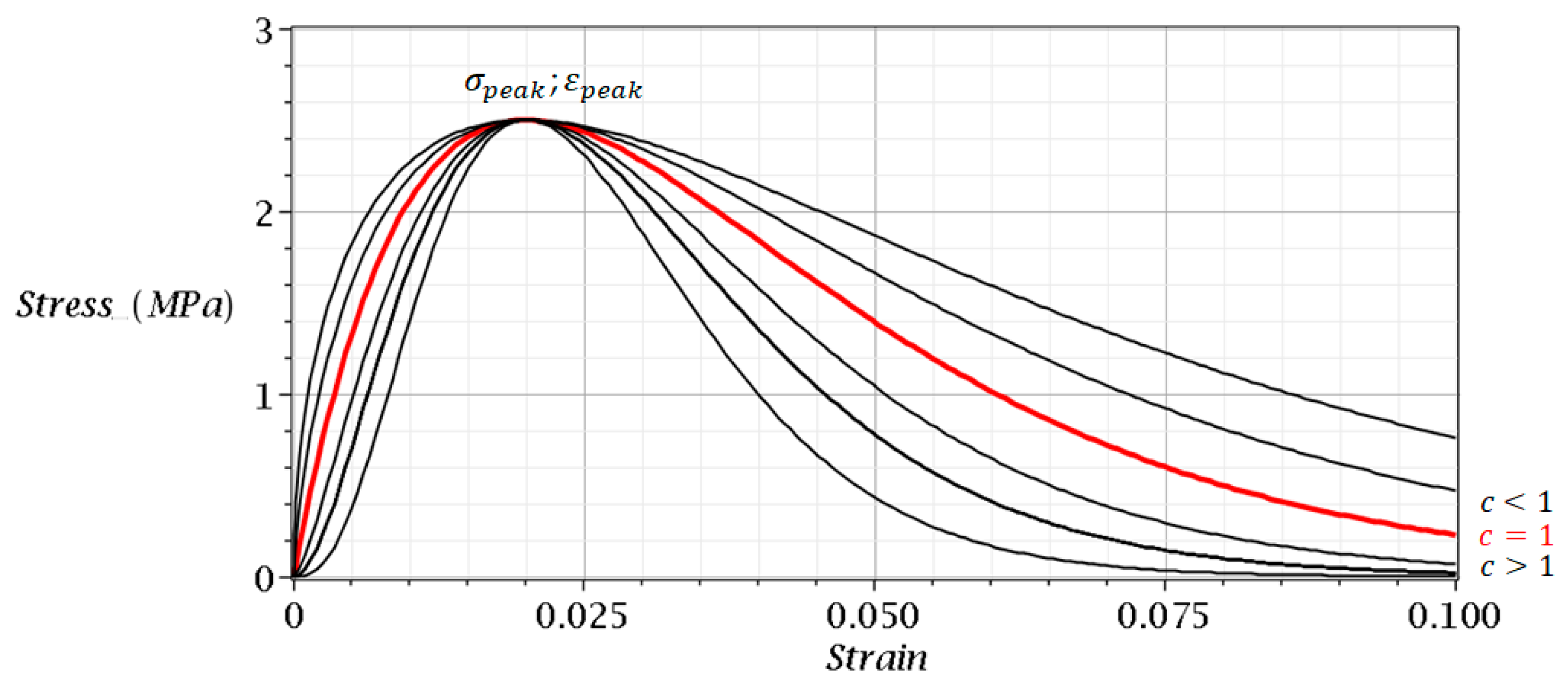
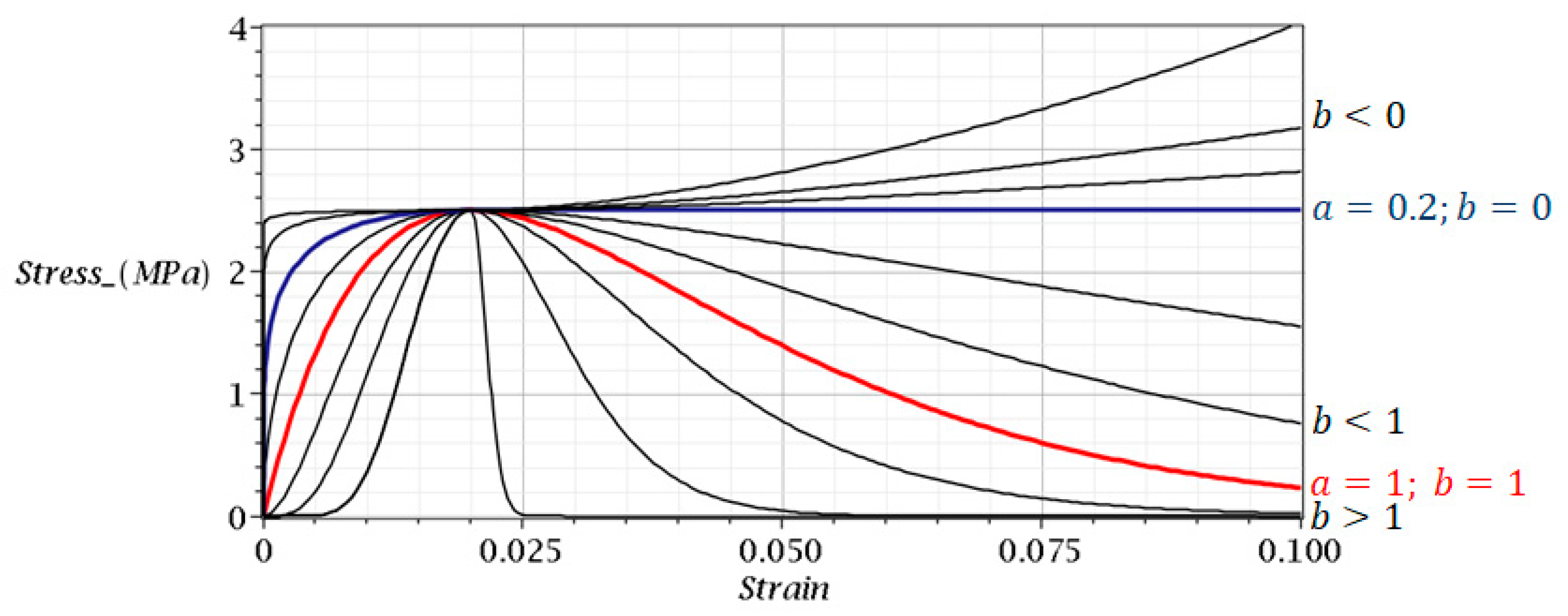
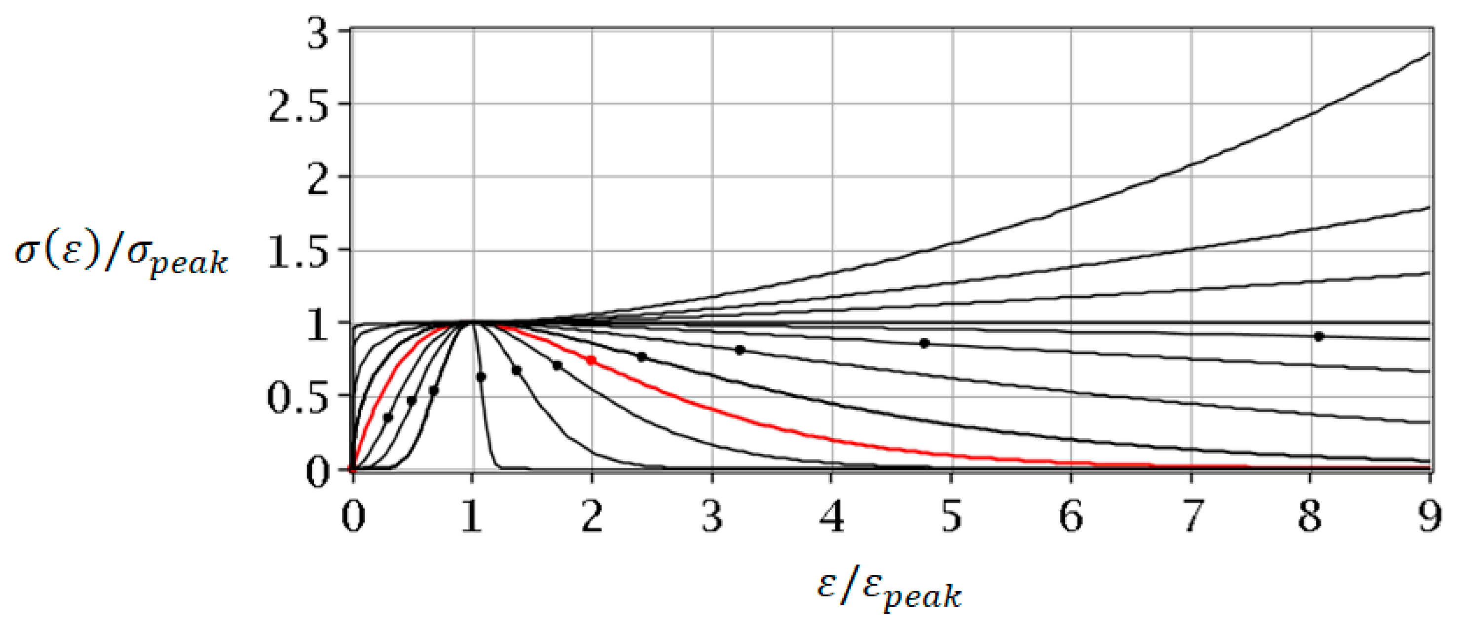
2.2. Model with Fully Separate Left and Right Branch Control

Let us represent parameter $c$ in the form $c=a+b$. Then, instead of (2), we write:

$$\sigma ={\sigma }_{peak}{\left(\frac{\epsilon }{{\epsilon }_{peak}}{e}^{\left(1-\frac{\epsilon }{{\epsilon }_{peak}}\right)}\right)}^{a+b}.$$

(4)

Let parameter $a$ refer only to the left branch and do not affect the right branch of the full curve$\sigma =\sigma \left(\epsilon \right)$; symmetrically, let parameter $b$ refer only to the right branch and do not affect the left branch of the same curve (4). At a point with coordinates ${\sigma }_{peak}$ and ${\epsilon }_{peak}$ on the left and right branches, both values of function $\sigma =\sigma \left(\epsilon \right)$ and derivatives $d\sigma /d\epsilon$ coincide, which is a necessary condition for correct connection of branches (Figure 1). The above conditions correspond to the equation, which can be written using the Heaviside function:

$$\sigma ={\sigma }_{peak}{\left(\frac{\epsilon }{{\epsilon }_{peak}}{e}^{\left(1-\frac{\epsilon }{{\epsilon }_{peak}}\right)}\right)}^{a \stackrel{=}{H}\left(1-\frac{\epsilon }{{\epsilon }_{peak}}\right)+b \stackrel{=}{H}\left( \frac{\epsilon }{{\epsilon }_{peak}}-1\right) }.$$

(5)

Heaviside function $\stackrel{=}{H} \left(x\right)=1$, if $x\ge 0;$ $\stackrel{=}{H} \left(x\right)=0$, if $x<0$. Taking into account that $\stackrel{=}{H} \left(x\right)=1-\stackrel{=}{H} \left(-x\right)$, let us write down:

$$\stackrel{=}{H}\left(\frac{\epsilon }{{\epsilon }_{peak}}-1\right)=b\left(1-\stackrel{=}{H}\left(1-\frac{\epsilon }{{\epsilon }_{peak}} \right)\right).$$

(6)

Using (6), transform Equation (5) to the form (7):

$$\sigma ={\sigma }_{peak}{\left(\frac{\epsilon }{{\epsilon }_{peak}}{e}^{\left(1-\frac{\epsilon }{{\epsilon }_{peak}}\right)}\right)}^{\left(a-b\right) \stackrel{=}{H}\left(1-\frac{\epsilon }{{\epsilon }_{peak}}\right)+b }.$$

(7)

Thus, we justified Equation (7) and, thus, based on the methodology of analysis and synthesis, we obtained a new model of the behavior of brittle materials, which is a modification of the models of Blagojevich et al. [17] and Stojkovic et al. [15]. It should be noted that the model whose mathematical description is represented by Equation (7) belongs to the same class of models whose development history is given in the above studies [15,16,17].

The Heaviside function in Equations (5) and (7) automatically switches parameters $a$ and $b$ while excluding their mutual influence. From a physical point of view, Equation (5) describes each of the branches of the full curve by the Blagojevich Equation (2). As in the models discussed above, parameters $a$ and $b$ can be obtained by fitting them to experimental data. Equation (7) is a mathematical description of the proposed modification of models (2) and (3).

Figure 2, as an addition to Figure 1, shows examples of curves $\sigma =\sigma \left(\epsilon \right)$ for some values of $a$ and $b$ at ${\sigma }_{peak}=2.5$ MPa and${\epsilon }_{peak}=0.02$.

Figure 2 shows that Equation (7) can be used to model the behavior of materials with the asymmetric stress–strain curves typical of brittle materials. In addition, the ascending branch at $b<0$ indicates some possibilities for modeling materials with strengthening, but this aspect is not considered in the current study. Since both branches of the full curve in model (7) can be ascending (Figure 2), we use the terms “left branch” and “right branch” instead of the terms “ascending branch” and “descending branch”, which are similar in meaning.

3. Results and Comments

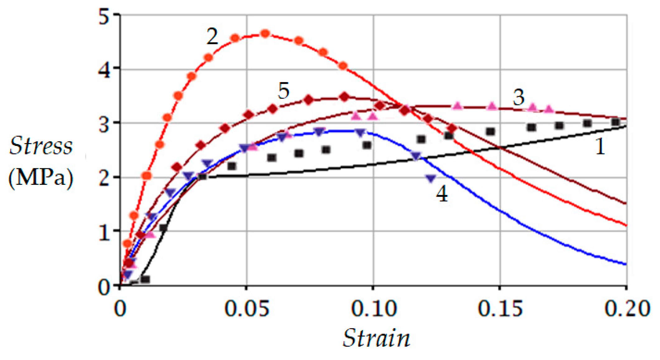
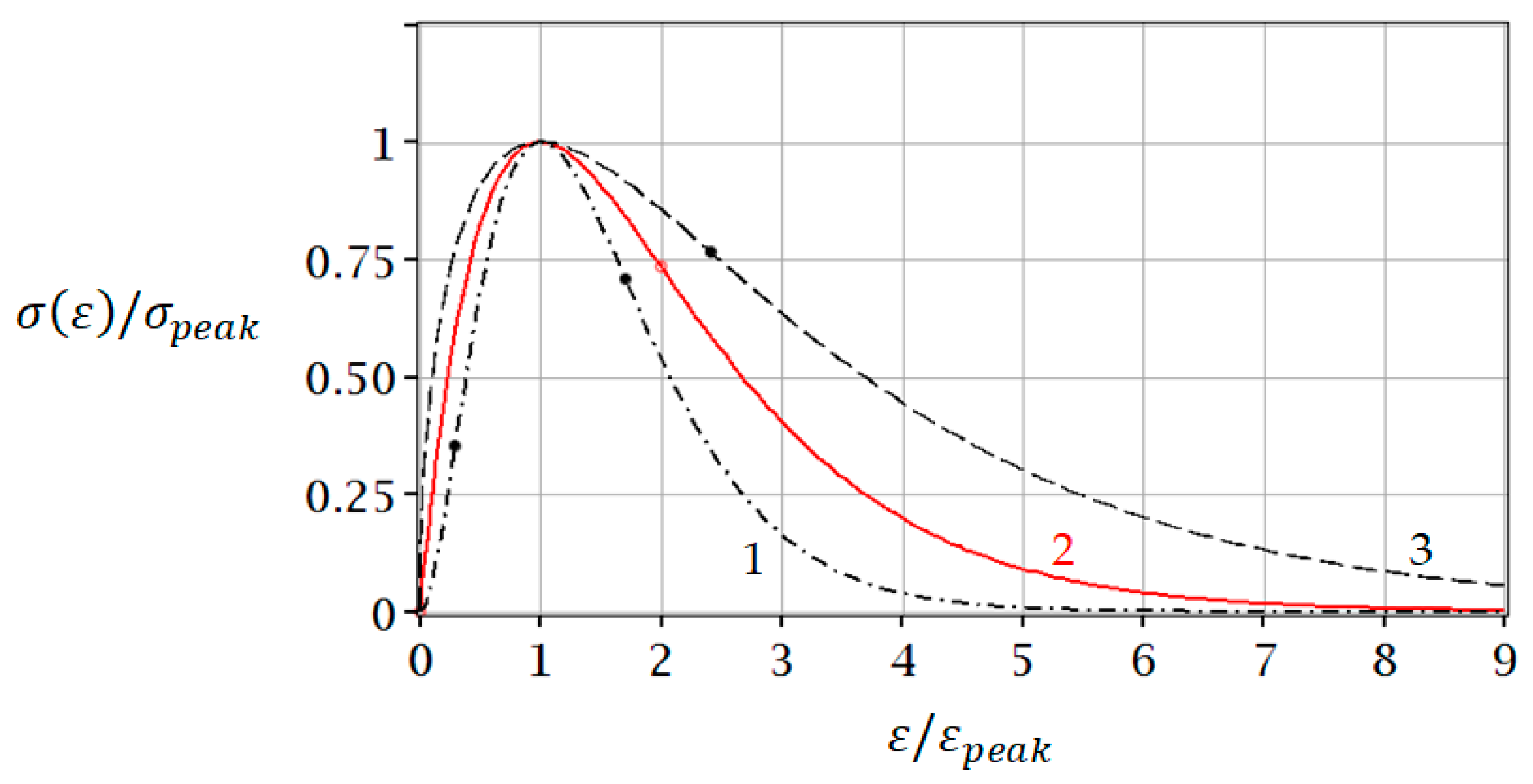
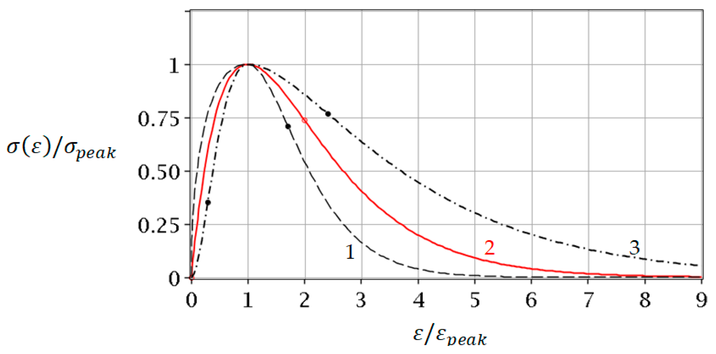
3.1. Comparison with Experimental Data Known from the Literature

To verify model (7), the experimental data for frozen ground (−10 °C) under compression detailed in the article [19] were used. The characteristics of the samples from the mentioned article and the suggested values of parameters $a$ and $b$ (7) are given in

Table 1. Characteristics of frozen soil samples and parameters $a$ and $b$.

Number	Soil	${\mathit{\sigma }}_{\mathit{p}\mathit{e}\mathit{a}\mathit{k}}$ (MPa)	${\mathit{\epsilon }}_{\mathit{p}\mathit{e}\mathit{a}\mathit{k}}$	$\mathit{a}$	$\mathit{b}$
1	Mucky soil *	2.00 *	0.0335 *	4.00	−0.12
2	Medium coarse sand *	4.61 *	0.0560 *	1.00	1.10
3	Clay *	3.29 *	0.1226 *	0.85	0.50
4	Calcareous clay *	2.84 *	0.0914 *	0.80	5.00
5	Sandy clay *	3.45 *	0.0905 *	0.80	2.00

* adapted after Chen et al. [19].

. The experimental and model data are shown in Figure 3.

Figure 3 shows that model (7) correctly reflects the compression behavior of frozen soils, but a better fit is obtained for sandy soil. Of practical (or innovative) interest may be the relationship between parameters $a$ and $b$ (Table 1) and the features of the stress–strain curves (Figure 3).

For frozen sand, parameter $a=1$ (Table 1), but the soil contains clay, so $a<1$. A comparison of samples 3 and 5 shows that sand in combination with clay increases the strength of the soil but reduces its plasticity; for clay parameter $b=0.5$, but for clayey soil containing sand $b>1$. Thus, parameters $a$ and $b$ correlate with the geomechanical characteristics of soils and the clarification of this relationship may be the subject of further research.

3.2. Predicting Values ${\sigma }_{peak}$ and ${\epsilon }_{peak}$

3.2.1. Prediction Methodology

The values ${\sigma }_{peak}$ and ${\epsilon }_{peak}$ are needed to model the behavior of brittle material (Figure 1). These values can be determined experimentally by bringing the sample or structure to failure. However, such direct determination of ${\sigma }_{peak}$ and ${\epsilon }_{peak}$ may be unacceptable if controlled failure of the actual test object is not technically possible or economically feasible. In such cases, indirect measurements are used, the methodology of which is discussed, for example, in [20].

Consider the method of indirect determination of ${\sigma }_{peak}$ and ${\epsilon }_{peak}$, if the experimental values at three points of the left branch of the full curve are known, i.e., ${\sigma }_{\left(1\right)}$, ${\epsilon }_{\left(1\right)}$, ${\sigma }_{\left(2\right)}$, ${\epsilon }_{\left(2\right)}$, ${\sigma }_{\left(3\right)}$, and ${\epsilon }_{\left(3\right)}$, such that ${\sigma }_{\left(1\right)}<{\sigma }_{\left(2\right)}<{\sigma }_{\left(3\right)}<{\sigma }_{peak}$ and ${\epsilon }_{\left(1\right)}<{\epsilon }_{\left(2\right)}<{\epsilon }_{\left(3\right)}<{\epsilon }_{peak}$, this means that we consider the left branch of the full curve (7) if $\epsilon /{\epsilon }_{peak}<1$ and$\stackrel{=}{H}\left(1-\epsilon /{\epsilon }_{peak}\right)=1$. Let us write down the left branch equation of the full curve:

$$\sigma ={\sigma }_{peak}{\left(\frac{\epsilon }{{\epsilon }_{peak}}{e}^{\left(1-\frac{\epsilon }{{\epsilon }_{peak}}\right)}\right)}^{ a }.$$

(8)

Substitute $\sigma ={\sigma }_1$ and $\epsilon ={\epsilon }_1$ in (8) and from the resulting equality we express ${\sigma }_{peak}$:

$${\sigma }_{peak}={\sigma }_{\left(1\right)}{\left(\frac{{\epsilon }_{peak}}{{\epsilon }_{\left(1\right)}}{e}^{ \left(1-\frac{{\epsilon }_{\left(1\right)}}{{\epsilon }_{peak}}\right)}\right)}^{-a} .$$

(9)

Similarly, substitute $\sigma ={\sigma }_2$ and $\epsilon ={\epsilon }_2$ into (8) and express ${\sigma }_{peak}$:

$${\sigma }_{peak}={\sigma }_{\left(2\right)}{\left(\frac{{\epsilon }_{peak}}{{\epsilon }_{\left(2\right)}}{e}^{-\left(1-\frac{{\epsilon }_{\left(2\right)}}{{\epsilon }_{peak}}\right)}\right)}^{-a} .$$

(10)

From Equations (9) and (10), it is possible to express ${\epsilon }_{peak}$:

$${\epsilon }_{peak}=\frac{a\left({\epsilon }_{\left(2\right)}-{\epsilon }_{\left(1\right)}\right)}{ln\frac{{\sigma }_{\left(1\right)}{\epsilon }_{\left(2\right)}^a}{{\sigma }_{\left(2\right)}{\epsilon }_{\left(1\right)}^a}} .$$

(11)

By analogy, we write:

$${\epsilon }_{peak}=\frac{a\left({\epsilon }_{\left(3\right)}-{\epsilon }_{\left(1\right)}\right)}{ln\frac{{\sigma }_{\left(1\right)}{\epsilon }_{\left(3\right)}^a}{{\sigma }_{\left(3\right)}{\epsilon }_{\left(1\right)}^a}} .$$

(12)

From Equations (11) and (12), we find parameter $a$:

$$a=\frac{ {\epsilon }_{\left(1\right)}\ln \frac{{\sigma }_{\left(3\right)}}{{\sigma }_{\left(2\right)}}-{\epsilon }_{\left(2\right)}\ln \frac{{\sigma }_{\left(3\right)}}{{\sigma }_{\left(1\right)}}+{\epsilon }_{\left(3\right)}\ln \frac{{\sigma }_{\left(2\right)}}{{\sigma }_{\left(1\right)}} }{{\epsilon }_{\left(1\right)}\ln \frac{{\epsilon }_{\left(3\right)}}{{\epsilon }_{\left(2\right)}}+{\epsilon }_{\left(2\right)}\ln \frac{{\epsilon }_{\left(1\right)}}{{\epsilon }_{\left(3\right)}}+{\epsilon }_{\left(3\right)}\ln \frac{{\epsilon }_{\left(2\right)}}{{\epsilon }_{\left(1\right)}}} .$$

(13)

Having calculated parameter$a$, we find ${\sigma }_{peak}$ ((9) or (10)). To calculate${\sigma }_{peak}$, parameter $b$ is not required. The values of parameter $b$ can be determined empirically.

3.2.2. Prediction Algorithm

Based on the obtained ratios (8)–(13), it is possible to construct the following algorithm for predicting the values of ${\sigma }_{peak}$ and ${\epsilon }_{peak}$:

• Initial data: ${\sigma }_{\left(1\right)}<{\sigma }_{\left(2\right)}<{\sigma }_{\left(3\right)}<{\sigma }_{peak}$ and ${\epsilon }_{\left(1\right)}<{\epsilon }_{\left(2\right)}<{\epsilon }_{\left(3\right)}<{\epsilon }_{peak}$.
• Parameter $a$ (13) is calculated.
• ${\epsilon }_{peak}$ (12) is calculated.
• ${\sigma }_{peak}$ (10) is calculated.

Let us pay attention to the algorithm features:

• The accuracy of the initial data should be high enough, because the results of calculations are sensitive to errors of rounding and experiment. However, this is not critical, because modern test machines provide high accuracy of experimental data [21,22].
• If the dependence $\sigma \left(\epsilon \right)$ is linear, then, for example, ${\sigma }_{\left(1\right)}{\epsilon }_{\left(2\right)}={\sigma }_{\left(2\right)}{\epsilon }_{\left(1\right)}$ (11) and theoretically${\epsilon }_{peak}=\infty$, ${\sigma }_{peak}=\infty$, which does not correspond to the physical meaning of task.

3.2.3. Limiting the Algorithm Scope

Limitation of the scope: the left branch of the complete curve σ(ε) must not contain an inflection point; this condition is satisfied if $0<a\le 1$. The analytical expression of this restriction can be obtained from equation $d^2\sigma /d{\epsilon }^2=0$. Taking into account Function (8), it follows that coordinate $\mathsf{\epsilon }$ of the inflection point of the left and right branches of the complete curve $\sigma \left(\epsilon \right)$ (7) is related to ${\epsilon }_{peak}$, respectively, by the relations:

$$\epsilon =\frac{\left(\sqrt{a}-1\right)}{\sqrt{a}}{\epsilon }_{peak} \mathrm{and} \epsilon =\frac{\left(\sqrt{b}+1\right)}{\sqrt{b}}{\epsilon }_{peak}$$

(14)

In addition to Figure 2, a general understanding of the inflection points of curves $\sigma \left(\epsilon \right)/{\sigma }_{peak}$ depending on parameters $a$ and $b$ can be obtained from Figure 4 (solid circles). For a more detailed consideration, the normalized coordinates ($\epsilon /{\epsilon }_{peak}$) of the inflection points of the left and right branches (14) for some values of parameters $a$ and $b$ are given in

Table 2. Normalized coordinates$\left(\epsilon /{\epsilon }_{peak}\right)$ of inflection points.

$\mathit{a}$	$\mathit{\epsilon }/{\mathit{\epsilon }}_{\mathit{p}\mathit{e}\mathit{a}\mathit{k}}$	$\mathit{b}$	$\mathit{\epsilon }/{\mathit{\epsilon }}_{\mathit{p}\mathit{e}\mathit{a}\mathit{k}}$
1.000	0.000	0.125	3.828
2.000	0.293	0.250	3.000
3.000	0.423	1.000	2.000
4.000	0.500	2.000	1.500
5.000	0.553	4.000	1.447

.

3.2.4. Example of the Algorithm Application

Before considering the example, let us explain that any three points on the left branch of the full curve (7) can be selected as the above points 1, 2, and 3 (Figure 5); i.e., there are infinitely many choices of these points. The following example uses experimental data from Chen et al. [19]. The initial data (${\epsilon }_{\left(1\right)}$, ${\epsilon }_{\left(2\right)}$,${\epsilon }_{\left(3\right)}$, ${\sigma }_{\left(1\right)}$, ${\sigma }_{\left(2\right)}$, and ${\sigma }_{\left(3\right)}$) and calculation results (${\epsilon }_{peak}$ and ${\sigma }_{peak}$) for curve 2 (Figure 3) are given in

Table 3. Initial data and calculation results.

Point Number	$\mathit{\epsilon }$	$\mathit{\sigma }$ (MPa)	$\mathit{a}$	${\mathit{\epsilon }}_{\mathit{p}\mathit{e}\mathit{a}\mathit{k}}$	${\mathit{\sigma }}_{\mathit{p}\mathit{e}\mathit{a}\mathit{k}}$ (MPa)
Initial data:			Calculation results:
1	0.004855	1.0278
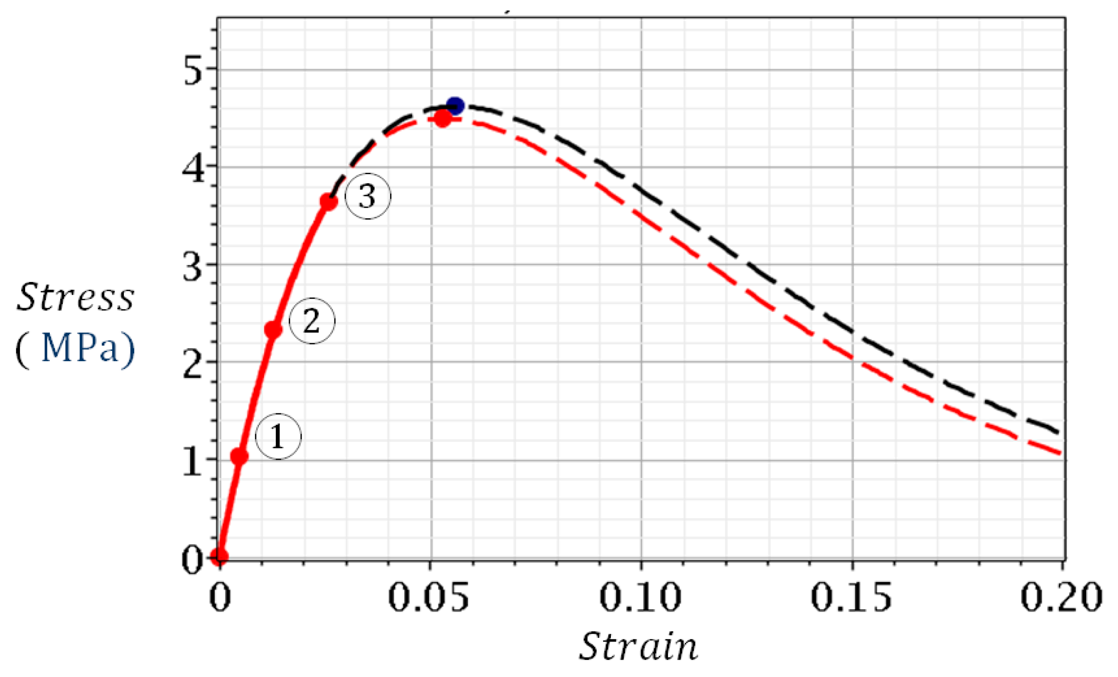
2	0.012923	2.3224	0.99	0.053 (105%)	4.49 (97%)
3	0.026087	3.6364
The experiment 1:				0.056 (100%)	4.61 (100%)

¹ The results of the experiment [19] were taken as 100%.

.

Commenting on Table 3, let us pay attention to the possible variations in the simulation results due to the influence of random factors, which usually appear in the testing process. Namely, using Equations (9) and (10), we obtain the values of ${\sigma }_{peak}$, respectively, as 4.54 and 4.49 MPa. In this case, small deviations from the average value (4.51 MPa) can be considered as an indicator of the stability of the computational circuit. From the physical point of view, the small deviations from the experimental data confirm the adequacy of the modeling methodology and the reliability of the simulation results.

Thus, Table 3 and Figure 3 and Figure 5 show that model (7) and the technique for predicting peak ${\sigma }_{peak}$ and ${\epsilon }_{peak}$ values can be considered as verified. Nevertheless, further research is needed to justify the limitations on the scope of the proposed model.

4. Discussion

In addition to the above remarks on the calculations, we note the following: The most important result of this work is the algorithm for predicting the carrying capacity of brittle material, which is based on previous studies of analytical models [15,16,17]. Attempts to justify such a model from a physical point of view and its mathematical description are also reflected in [18]. However, an analytical model for predicting the bearing capacity of brittle material using incomplete experimental data could not be found. This paper proposes a new model (5)–(13) and shows that the simulation results are consistent with experimental data found in the literature and provide acceptable accuracy for the predicted values of ${\sigma }_{peak}$ and ${\epsilon }_{peak}$ (Figure 3 and Figure 5; Table 3).

The initial data for the model (5)–(13) do not contain the characteristics of the granulometric composition, strength and other physical and mechanical properties of the material under study. These properties may remain unknown, but their influence is indirectly taken into account by means of ${\sigma }_{peak}$ and ${\epsilon }_{peak}$, i.e., the “black box” methodology is used, when instead of the properties and relationships of the components of the system, the reaction of the system as a whole to changing conditions is studied [23]. Thus, the model (5)–(13) is quite universal, but additional research is needed to determine the scope of the rational application of the model.

The main result of this study was obtained through the asymmetric independent control of the right and left branches of the full load–strain curve. At the level of model (5)–(7), such control is realized through decomposition (or splitting) of parameter $c$ in the Blagojevich model (2) to two parameters: $c=a+b$ ((5)–(7)). In this case, from the geometrical point of view, the right and left branches of the full load-deformation curve are correctly related to the values of the function and its derivatives at the point of extremum (peak of the curve). Justifying the necessity of independent control of the right and left branches of the total load–displacement curve from the physical point of view, we note that under loading, micro- and meso-cracks gradually appear and grow in a brittle material, which causes the brittle properties of the material to differ in the pre-peak and post-peak stages of loading (as reflected in a large number of publications [24]). Accordingly, using only one equation, it is difficult to account for the properties at pre- and post-peak loading stages. However, this small obstacle was overcome by applying the Heaviside function in the model proposed above (4)–(14). Thus, a physically adequate and mathematically correct solution to this issue has been found, which is confirmed by agreement with the experimental data (Figure 3 and Figure 5). A visual representation of the symmetric and asymmetric control of the right (upward) and left (downward) branches of the full curve, in addition to Figure 4, can be obtained from the graphs in Figure 6 and Figure 7.

All of the curves in Figure 1, Figure 2 and Figure 4 intersect at a point that corresponds to the peak load. These figures, in analogy with [15,17], show that the model does not exclude the possibility of different trajectories from zero load to the same peak value. The curves with different peak values are shown in Figure 3 (curves 2–5).

The expediency of continuing research is indicated by a certain analogy of stress–strain curves (Figure 1, Figure 2 and Figure 3) for concrete [25,26], rock materials [21,22], geopolymers [27,28,29,30], frozen soils, and other brittle materials [31,32,33,34]. The focus of future research on the topic may be on the right branch of the full stress–strain (or load–displacement) curve. The need to focus on this issue is explained by the fact that brittle materials are destroyed on the descending branch of the full stress–strain curve, as shown in Figure 3, as well as in studies [21,22].

Concluding the discussion, we note that the relations (4)–(14) discussed above are formulated in terms of stress–strain. In this case, stresses directly characterize the external load on the sample; strains characterize the change in the size of the sample (as a whole). Thus, model (4)–(14) can be called a load–displacement model formulated in terms of stress–strain. Based on the methodology used in this paper, it is possible to develop a model without referring to stress–strain terms, i.e., using only the values of the external load and the corresponding displacements [35]. Using the characteristics of the external impact and the geometry of the sample as input data, it is possible to determine internal stresses and strains at any point of the sample, using, for example, finite element or discrete element methods [7,36], which is beyond the scope of this work.

5. Conclusions

A review of one class of analytical models used to assess the behavior of brittle materials under loading was carried out here. A distinctive feature of these models is the use of only one equation for the mathematical description of the full stress–strain (or load–displacement) curve. The necessity of developing a new model of the same class, providing the possibility of analytical prediction of the maximum load using experimental data for the pre-peak stage of the deformation of brittle material, is substantiated. The advantage of analytical models compared to numerical modeling is the reduction in the cost of modeling and the expansion of the possibilities of applied research concerning the behavior of brittle materials in engineering structures in order to increase their safety and economic efficiency.

In this work, Equation (7) is substantiated and, thus, based on the methodology of analysis and synthesis, a new model of the behavior of brittle materials is obtained, which is a modification of the models of Blagojevich et al. [17] and Stojkovic et al. [15]. It should be noted that the model whose mathematical description is represented by Equation (7) belongs to the same class of models whose development history is given in the studies [15,16,17].

A methodology has been developed for applying the developed model to predict peak load values using only pre-peak load values and corresponding deformations.

The developed behavior model of brittle materials and the method of peak load prediction were tested for sandy soils using experimental data known from the literature.

A limitation for the scope of application of the developed method for predicting peak loads is determined, namely that the ascending branch of the load–strain curve should not contain inflection points.

The focus of future research on the topic may be on the right branch of the full stress–strain curve. The need to focus on this issue is explained by the fact that brittle materials are destroyed on the descending branch of this curve.

References

- Pan, Z.; Ma, R.; Wang, D.; Chen, A. A review of lattice type model in fracture mechanics: Theory, applications, and perspectives. Eng. Fract. Mech. 2018, 190, 382–409. [Google Scholar] [CrossRef]
- de Borst, R. Fracture in quasi-brittle materials: A review of continuum damage-based approaches. Eng. Fract. Mech. 2002, 69, 95–112. [Google Scholar] [CrossRef]
- Pugno, N.M. Dynamic quantized fracture mechanics. Int. J. Fract. 2006, 140, 159–168. [Google Scholar] [CrossRef]
- Zheng, B.; Li, T.; Qi, H.; Gao, L.; Liu, X.; Yuan, L. Physics-informed machine learning model for computational fracture of quasi-brittle materials without labelled data. Int. J. Mech. Sci. 2022, 223, 107282. [Google Scholar] [CrossRef]
- Cervera, M.; Barbat, G.B.; Chiumenti, M.; Wu, J.Y. A Comparative Review of XFEM, Mixed FEM and Phase-Field Models for Quasi-brittle Cracking. Arch. Comput. Methods Eng. 2022, 29, 1009–1083. [Google Scholar] [CrossRef]
- Zhu, R.; Gao, H.; Zhan, Y.; Wu, Z.-X. Construction of Discrete Element Constitutive Relationship and Simulation of Fracture Performance of Quasi-Brittle Materials. Materials 2022, 15, 1964. [Google Scholar] [CrossRef]
- Chen, H.; Zhang, Y.X.; Zhu, L.; Xiong, F.; Liu, J.; Gao, W. A Particle-Based Cohesive Crack Model for Brittle Fracture Problems. Materials 2020, 13, 3573. [Google Scholar] [CrossRef]
- Ying, J.; Guo, J. Fracture Behaviour of Real Coarse Aggregate Distributed Concrete under Uniaxial Compressive Load Based on Cohesive Zone Model. Materials 2021, 14, 4314. [Google Scholar] [CrossRef]
- Hurley, R.C.; Hogan, J.D. Workshop on Mathematical Challenges in Brittle Material Failure. J. Dyn. Behav. Mater. 2020, 6, 14–23. [Google Scholar] [CrossRef]
- Sánchez, M.; Cicero, S.; Arrieta, S.; Martínez, V. Fracture Load Predictions in Additively Manufactured ABS U-Notched Specimens Using Average Strain Energy Density Criteria. Materials 2022, 15, 2372. [Google Scholar] [CrossRef] [PubMed]
- Kovalchenko, A.M. Studies of the ductile mode of cutting brittle materials (A review). J. Superhard Mater. 2013, 35, 259–276. [Google Scholar] [CrossRef]
- Oucif, C.; Mauludin, L.M. Continuum Damage-Healing and Super Healing Mechanics in Brittle Materials: A State-of-the-Art Review. Appl. Sci. 2018, 8, 2350. [Google Scholar] [CrossRef]
- Iskander, M.; Shrive, N. Fracture of brittle and quasi-brittle materials in compression: A review of the current state of knowledge and a different approach. Theor. Appl. Fract. Mech. 2018, 97, 250–257. [Google Scholar] [CrossRef]
- Xiao, P.; Zhao, G.; Liu, H. Failure Transition and Validity of Brazilian Disc Test under Different Loading Configurations: A Numerical Study. Mathematics 2022, 10, 2681. [Google Scholar] [CrossRef]
- Stojković, N.; Perić, D.; Stojić, D.; Marković, N. New stress-strain model for concrete at high temperatures. Teh. Vjesn. 2017, 24, 863–868. [Google Scholar]
- Baldwin, R.; North, M.A. Stress-strain curves of concrete at high temperature-A review. Fire Saf. Sci. 1969, 785, 1. Available online: http://www.iafss.org/publications/frn/785/-1/view/frn_785.pdf (accessed on 12 October 2021).
- Blagojević, M.; Pešić, D.; Mijalković, M.; Glišović, S. Jedinstvena funkcija za opisivanje naprezanja i deformacije betona u požaru. Građevinar 2011, 63, 19–24. Available online: https://hrcak.srce.hr/clanak/96329 (accessed on 14 July 2022).
- Kolesnikov, G. Damage Function of a Quasi-Brittle Material, Damage Rate, Acceleration and Jerk during Uniaxial Compression: Model and Application to Analysis of Trabecular Bone Tissue Destruction. Symmetry 2021, 13, 1759. [Google Scholar] [CrossRef]
- Chen, J.; Wang, L.; Yao, Z. Physical and mechanical performance of frozen rocks and soil in different regions. Adv. Civ. Eng. 2020, 2020, 8867414. [Google Scholar] [CrossRef]
- Ancillao, A.; Tedesco, S.; Barton, J.; O’Flynn, B. Indirect Measurement of Ground Reaction Forces and Moments by Means of Wearable Inertial Sensors: A Systematic Review. Sensors 2018, 18, 2564. [Google Scholar] [CrossRef]
- Hou, P.Y.; Cai, M.; Zhang, X.W.; Feng, X.T. Post-peak Stress–Strain Curves of Brittle Rocks Under Axial and Lateral-Strain-Controlled Loadings. Rock Mech. Rock Eng. 2021, 147, 855–884. [Google Scholar] [CrossRef]
- Cai, M.; Hou, P.Y.; Zhang, X.W.; Feng, X.T. Post-peak stress–strain curves of brittle hard rocks under axial-strain-controlled loading. Int. J. Rock Mech. Min. Sci. 2021, 147, 104921. [Google Scholar] [CrossRef]
- Astbury, B.; Leeuw, F.L. Unpacking black boxes: Mechanisms and theory building in evaluation. Am. J. Eval. 2010, 31, 363–381. [Google Scholar] [CrossRef]
- Salviato, M.; Chau, V.T.; Li, W.; Bažant, Z.P.; Cusatis, G. Direct Testing of Gradual Postpeak Softening of Fracture Specimens of Fiber Composites Stabilized by Enhanced Grip Stiffness and Mass. J. Appl. Mech. 2016, 83, 111003. [Google Scholar] [CrossRef]
- Zhuang, J.; Xu, R.; Pan, C.; Li, H. Dynamic stress–strain relationship of steel fiber-reinforced rubber self-compacting concrete. Constr. Build. Mater. 2022, 344, 128197. [Google Scholar] [CrossRef]
- Zhang, L.; Cheng, H.; Wang, X.; Liu, J.; Guo, L. Statistical Damage Constitutive Model for High-Strength Concrete Based on Dissipation Energy Density. Crystals 2021, 11, 800. [Google Scholar] [CrossRef]
- Yadollahi, M.M.; Benli, A. Stress-strain behavior of geopolymer under uniaxial compression. Comput. Concr. 2017, 20, 381–389. [Google Scholar] [CrossRef]
- Wang, H.; Li, H.; Yan, F. Synthesis and mechanical properties of metakaolinite-based geopolymer. Colloids Surf. A Physicochem. Eng. Asp. 2005, 268, 1–6. [Google Scholar] [CrossRef]
- Davidovits, J. Geopolymer: Man-made rocks geosynthesis and the resulting development of very early high strength cement. J. Mat. Educ. 1994, 16, 91–139. [Google Scholar]
- Dal Poggetto, G.; D’Angelo, A.; Catauro, M.; Barbieri, L.; Leonelli, C. Recycling of Waste Corundum Abrasive Powder in MK-Based Geopolymers. Polymers 2022, 14, 2173. [Google Scholar] [CrossRef]
- Kolesnikov, G.; Gavrilov, T. Sandstone Modeling under Axial Compression and Axisymmetric Lateral Pressure. Symmetry 2022, 14, 796. [Google Scholar] [CrossRef]
- Wang, H.; Wu, Y.; Wei, M.; Wang, L.; Cheng, B. Hysteretic Behavior of Geopolymer Concrete with Active Confinement Subjected to Monotonic and Cyclic Axial Compression: An Experimental Study. Materials 2020, 13, 3997. [Google Scholar] [CrossRef] [PubMed]
- Abdellah, M.Y.; Zuwawi, A.-R.; Azam, S.A.; Hassan, M.K. A Comparative Study to Evaluate the Essential Work of Fracture to Measure the Fracture Toughness of Quasi-Brittle Material. Materials 2022, 15, 4514. [Google Scholar] [CrossRef] [PubMed]
- Kolesnikov, G. Analysis of Concrete Failure on the Descending Branch of the Load-Displacement Curve. Crystals 2020, 10, 921. [Google Scholar] [CrossRef]
- Katarov, V.; Syunev, V.; Kolesnikov, G. Analytical Model for the Load-Bearing Capacity Analysis of Winter Forest Roads: Experiment and Estimation. Forests 2022, 13, 1538. [Google Scholar] [CrossRef]
- Li, Z. A Numerical Method for Applying Cohesive Stress on Fracture Process Zone in Concrete Using Nonlinear Spring Element. Materials 2022, 15, 1251. [Google Scholar] [CrossRef] [PubMed]