Article

Transient Propagation of Longitudinal and Transverse Waves in Cancellous Bone: Application of Biot Theory and Fractional Calculus

1
Laboratory of Theoretical Physics, Faculty of Physics, University of Science and Technology Houari-Boumediene, BP 32 El Alia, Bab Ezzouar 16111, Algeria
2
Aix Marseille Univ, CNRS, Centrale Marseille, LMA UMR 7031, Laboratory of Mechanics and Acoustics, CEDEX 20, 13402 Marseille, France
3
Materials Physics Laboratory, Faculty of Physics, University of Science and Technology Houari-Boumediene, BP 32 El Alia, Bab Ezzouar 16111, Algeria
4
Department of Physics and Materials Science, Maseno University, Maseno 40105, Kenya
5
Laboratoire d’Acoustique de l’Université du Mans (LAUM), UMR 6613, Institut d’Acoustique, CNRS, Le Mans Université, Avenue O. Messiaen, CEDEX 09, 72085 Le Mans, France
*
Author to whom correspondence should be addressed.
Symmetry 2022, 14(10), 1971; https://doi.org/10.3390/sym14101971
Submission received: 1 August 2022 / Revised: 9 September 2022 / Accepted: 14 September 2022 / Published: 21 September 2022

Abstract

:
In this paper, the influence of the transverse wave on sound propagation in a porous medium with a flexible structure is considered. The study is carried out in the time domain using the modified Biot theory obtained by the symmetry of the Lagrangian (invariance by translation and rotation). The viscous exchanges between the fluid and the structure are described by fractional calculus. When a sound pulse arrives at normal incidence on a porous material with a flexible structure, the transverse waves interfere with the longitudinal waves during propagation because of the viscous interactions that appear between the fluid and the structure. By performing a calculation in the Laplace domain, the reflection and transmission operators are derived. Their time domain expressions depend on the Green functions of the longitudinal and transverse waves. In order to study the effects of the transverse wave on the transmitted longitudinal waves, numerical simulations of the transmitted waves in the time domain by varying the characteristic parameters of the medium are realized whether the transverse wave is considered or not.

1. Introduction

Osteoporosis is defined as a sickness that affects the bones, and to understand it, an overview of the structure of bone tissues is necessary. Bones are in perpetual renewal; this phenomenon is called bone remodeling: constant construction of new tissue and destruction of old tissue. In osteoporosis, biochemical and hormonal changes occur and affect this balance. The bone is, therefore, considerably weakened by reductions in its tissue and mass [1], a fragility that is increased tenfold when the contribution of bone minerals is reduced [2,3,4]. Therefore, there is a growing need for improved diagnosis and management of osteoporosis. Indeed, the sooner the disease is detected, the more effective the care can be.
As it is known, bone is an inhomogeneous porous material [5,6,7,8,9] and the determination of its characteristics by means of ultrasound techniques can be a game-changer in the diagnosis of osteoporosis since its elastic properties affect acoustic propagation. Within this context, several studies have been conducted on cancelous and trabecular bone [10,11,12,13]. There are ultrasonic methods that rely on the speed of sound and the broadband attenuation of a single wave to estimate the different stages of osteoporosis, but the poroelastic nature of the bone generates two types of waves during the propagation of the acoustic wave in the bone. The most appropriate theory for the study of acoustic wave propagation in porous media such as trabecular bone is the Biot theory [14,15,16,17,18,19,20,21,22,23,24,25,26,27]. This theory [14,15,16,17,18,19,20,21,22,23,24,25,26,27] has been proven to be a very advantageous model for the description of wave propagation in porous media saturated with fluids; it takes into account the movements of the solid and fluid phases, and through the mass, elastic, and viscous couplings, the interaction between these two phases is considered. Its main success lies in the prediction of the existence of three waves in a porous material subjected to external stress: two longitudinal waves and a transverse wave. The first compressional wave has the highest speed and is called the “fast wave”, while the second compressional wave has a lower speed and is called the “slow wave”.
Because of its very general and rather fundamental character, the Biot theory has been used widely in the field of petroleum exploration and geoscientific testing, but many have also applied it to the study of bone structures [14,15,28,29,30,31]. McKelvie [28,31] qualitatively predicted that, for cancelous bone, attenuation is related to ultrasound frequency. The second compressional wave with a lower velocity was reported in the studies by Lakes, Yoon, and Katz [32] on wet human and bovine cortical bone. The connection between porosity and longitudinal wave velocities and the relevance of the presence of these two waves to bone characterization were demonstrated by Hosokawa and Otani [14] in their studies of cancelous bone. By implementing the concepts of dynamic tortuosity, permeability, and viscous characteristic length, in 1987, Johnson et al. [33] made a major input to the study of porous media.
The modified Biot theory has been used to study the transmission and reflection of acoustic waves for different media in the frequency domain [34,35,36,37,38,39,40,41,42]. In order to offer an alternative to the frequency methods, Fellah and Depollier [43,44] have proposed a temporal approach [43,44,45,46,47,48,49,50,51,52] that allows the phenomena that follow the propagation of acoustic waves in porous media to be seen from a different angle. The viscous fluid/structure interactions are described using fractional calculus, which has been proven to be a well-adapted tool to describe the dispersion effects that develop when a wave passes in a saturated porous medium. Fractional derivatives and integrals [53,54,55,56,57,58,59,60,61,62,63,64,65] have long been the focus of research in mathematics, but their use outside mathematics is only recent. Indeed, the fractional derivative was only used towards the end of the 1960s by Caputo [57,58,59] to describe dissipation phenomena in solids and, later, by Bagley and Torvik [60] to treat viscoelastic materials, but the most significant contribution in the field of acoustics remains the one made by Matignon [61]. The reflection and transmission operators have been established as a result to external solicitation of a saturated porous medium by a viscous fluid in the frequency domain for normal incidence by considering the three Biot waves instead of only the longitudinal waves, by Hodaei, Maghoul, and Popplewell [66].
The purpose of this article is to study, from a new perspective, the behavior of a porous medium subjected to an external load when the three Biot waves (i.e., the transverse wave in addition to the longitudinal waves) are considered. For that, we establish the expressions of the diffusion operators in the time domain while including the effect of the transverse wave; the fractional calculus as well as the Biot model modified by Johnson et al. [33] will be used. Numerical simulations are given for the transmitted signals, with shear being taken into account or not while applying a variation of the characteristic parameters of the porous medium. The effect of transverse waves as well as the sensitivity of the parameters are studied. The advantage of this model is that it presents a temporal modeling of the propagation by taking into account both longitudinal and transverse waves in normal incidence.

2. Modified Biot Theory

The displacements of the solid phase u and the fluid phase U are modeled via the Biot theory, where the equations of motion are given by the following:
ρ 11 2 u t 2 + ρ 12 2 U t 2 = P ( . u ) + Q ( . U ) N ( u ) , ρ 22 2 U t 2 + ρ 12 2 u t 2 = R ( . U ) + Q ( . u ) .
N is the shear modulus of the solid structure. P, Q, and R are the elastic coefficients of Biot; they are functions of the bulk modulus of the pore fluid K f , the bulk modulus of the elastic solid K s , the bulk modulus of the porous skeletal frame K b as well as of the porosity ϕ of the porous medium and are defined by the relations below:
P = 1 ϕ 1 ϕ K b K s K s + ϕ K s K f 1 ϕ K b K s + ϕ K s K f + 4 3 N , Q = 1 ϕ K b K s ϕ K s 1 ϕ K b K s + ϕ K s K f , R = ϕ 2 K s 1 ϕ K b K s + ϕ K s K f ,
K f , K s , and K b depend on the classical mechanical parameters, which are Young’s moduli, Poisson’s coefficients of the solid E s and ν s , and Poisson’s coefficients of the skeleton E b and ν b as follows:
K s = E s 3 1 2 ν s , K b = E b 3 1 2 ν b , N = E b 2 1 + ν b .
The coefficients ρ i j involved in the motion equations are mass coefficients. They have a density dimension and are linked to the skeleton-constituting solid density ρ s , which constitutes the skeleton, and to the fluid density ρ f by:
ρ 11 = 1 ϕ ρ s ρ 12 , ρ 22 = ϕ ρ f ρ 12 ,
The term ρ 12 expresses the fluid–structure inertial coupling. It appears as a contribution to the densities of the fluid and the solid because of the interactions between the fluid and the structure.
ρ 12 = ϕ ρ f α 1 ,
α is the tortuosity of the medium. When an acoustic wave crosses a fluid-saturated porous medium, it is attenuated. This attenuation is mainly due to the viscous exchanges that occur between the structure and the saturating fluid because of relative fluid/solid displacements, leading to a modification of the densities. The tortuosity becomes a function of the frequency and is called dynamic tortuosity α ω :
ρ 12 ω = ϕ ρ f α ω 1 , ρ 11 ω = 1 ϕ ρ s + ϕ ρ f α ω 1 , ρ 22 ω = ϕ ρ f + ϕ ρ f α 1 .
In order to estimate the fluid domain affected by these exchanges, the thickness of the viscous boundary layer δ = 2 η ω ρ 0 1 / 2 ( η fluid viscosity and ω angular frequency) is compared to a microscopic dimension characteristic of the medium such as the pore size “a”. In the high-frequency mode, the viscous boundary layer thickness is small compared to the pore size “a” i.e., if ( δ a 1 ). In this mode, the viscous effects take place only in a small fluid thickness, at the walls where the velocities are affected by the fluid/solid displacements. In the rest of the fluid volume, the fluid behaves like a perfect fluid.
In this case, the dynamic tortuosity takes the following form:
α ω α 1 + 2 Λ η j ω ρ f ,
This model was proposed by Johnson et al. [33]. It involves the tortuosity α and the viscous characteristic length Λ , a geometric parameter indicative of small pores, in the high-frequency limit and represents the thickness where viscous effects are important.
By replacing the new expressions for the mass coefficients in (6) where α ω is given by (7) in the system of Equation (1), the motion equations becomes the following:
ρ 11 ω 2 u t 2 + ρ 12 ω 2 U ( t ) t 2 = P ( . u ) + Q ( . U ) N ( u ) , ρ 22 ω 2 U t 2 + ρ 12 ω 2 u t 2 = R ( . U ) + Q ( . u ) .
This system is written neither in the time domain nor in the frequency domain, since the densities depend on the frequency and the derivatives are in the time domain. In the following section, we try to describe the above problem in the time domain.

3. Temporal Formulation of the Modified Biot Theory

In order to study the waves transmitted in the time domain through a porous medium, we focus on the temporal formulation of the Biot theory. To achieve this, we introduce the concept of the fractional derivative of order ν , the definition of which [56] is given by the following:
D ν x t = 1 Γ ( ν ) 0 t ( t u ) ν 1 x ( u ) d u ,
where ν is a real number and Γ is the Gamma function.
The high-frequency expression of the dynamic tortuosity includes the term 1 j ω , of which the time equivalent is a fractional derivative of order 1/2. Following the definition in (9), the expression of the response factor α takes the following expression in the time domain [43,49]:
α ˜ t = α δ t + 2 Λ η π ρ f t 1 2 ,
where δ ( t ) is the Dirac function. With this new expression of the dynamic tortuosity α ˜ t in the system of Equation (1), the equations of motion in the time domain take the following shape:
0 t ρ 11 ˜ t t 2 u ( t ) t 2 d t + 0 t ρ 12 ˜ ( t t ) 2 U ( t ) t 2 d t = P ( u ( t ) ) + Q ( . U ( t ) ) N ( u ( t ) ) , 0 t ρ 22 ˜ ( t t ) 2 U ( t ) t 2 d t + 0 t ρ 12 ˜ ( t t ) 2 u ( t ) t 2 d t = R ( . U ( t ) ) + Q ( u ( t ) ) ,
where the temporal operators ρ 11 ˜ , ρ 12 ˜ , and ρ 22 ˜ are obtained by replacing α ( ω ) in Equation () by its temporal equivalent α ˜ given by Equation (10).

3.1. Solution of the Motion Equations

According to Helmholtz’s theorem, a solution to the system in (11) has the following form:
u ( x , t ) = Φ s ( x , t ) + Ψ s ( x , t ) , U ( x , t ) = Φ f ( x , t ) + Ψ f ( x , t ) ,
where Φ s and Φ f are the scalar displacement potentials of the solid u and fluid U , respectively, and Ψ s and Ψ f are the vector potentials of u and U , respectively. The Biot equations of motion are linear, and it it is possible to look for the scalar and vector solutions separately.

3.1.1. Longitudinal Waves

In the case of the longitudinal wave, the contribution of scalar displacement potentials are obtained by substituting u ( x , t ) = Φ s ( x , t ) and U = Φ f ( x , t ) in the equations of motion, which gives
ρ 11 ρ 12 ρ 12 ρ 22 2 t 2 Φ s ( x , t ) Φ f ( x , t ) + a 1 1 1 1 3 2 t 3 2 Φ s ( x , t ) Φ f ( x , t ) = P Q Q R Δ Φ s ( x , t ) Φ f ( x , t ) ,
where a = 2 ϕ ρ f α Λ η ρ f 2 Δ is the Laplacian. The viscous effects are included in the fractional derivative term 3 2 t 3 2 . To solve this system of equations, we use the Laplace transform. The Biot equations are then written as follows:
Δ Φ s ˜ ( x , s ) Φ f ˜ ( x , s ) = M Φ s ˜ ( x , s ) Φ f ˜ ( x , s ) ,
where Φ s ˜ and Φ f ˜ are, respectively, the Laplace transform of Φ s and Φ f . We note that Φ s ˜ ( x , s ) is the Laplace transform of Φ s ( x , t ) defined by the following:
Φ s ˜ ( s ) = L Φ s ( t ) = 0 + exp ( s t ) Φ s ( t ) d t .
The matrix M is given by the following:
M = ( R ρ 11 Q ρ 12 ) s 2 + a s 3 2 ( R + Q ) ( R ρ 12 Q ρ 22 ) s 2 a s 3 2 ( R + Q ) ( P ρ 12 Q ρ 11 ) s 2 a s 3 2 ( P + Q ) ( P ρ 22 Q ρ 12 ) s 2 + a s 3 2 ( P + Q ) ,
with
R Q Q P = P Q Q R 1 = R P R Q 2 Q P R Q 2 Q P R Q 2 P P R Q 2 ,
R = R P R Q 2 , Q = Q P R Q 2 , P = P P R Q 2 .
The system is solved by finding the eigenvalues of the matrix M:
Δ Φ 1 ( x , s ) Φ 2 ( x , s ) = λ 1 ( s ) 0 0 λ 2 ( s ) Φ 1 ( x , s ) Φ 2 ( x , s ) .
This corresponds to the following equations:
2 Φ 1 ( x , s ) x 2 = λ 1 ( s ) Φ 1 ( x , s ) , 2 Φ 2 ( x , s ) x 2 = λ 2 ( s ) Φ 2 ( x , s ) ,
The solutions to the above are in the following form:
Φ 1 ( x , s ) = Φ 11 ( s ) e x λ 1 ( s ) + Φ 12 ( s ) e x λ 1 ( t ) ,
Φ 2 ( x , s ) = Φ 21 ( s ) e x λ 2 ( s ) + Φ 22 ( s ) e x λ 2 ( s ) .
The displacements of the solid and fluid are the linear combinations of the displacements due to the fast wave (first-type wave) characterized by the scalar potential Φ 1 ( x , s ) and the slow wave (second-type wave) characterized by the scalar potential Φ 2 ( x , s ) .
We associate the eigenvalues λ 1 ( s ) and λ 2 ( s ) with eigenvectors 1 , V 1 ( s ) and 1 , V 2 ( s ) , which link the fast and slow waves Φ 1 ( x , s ) and Φ 2 ( x , s ) to the solid and fluid waves Φ s ˜ ( x , s ) and Φ f ˜ ( x , s ) .
Φ s ˜ ( x , s ) Φ f ˜ ( x , s ) = 1 1 V 1 ( s ) V 2 ( s ) Φ 1 ( x , s ) Φ 2 ( x , s ) .
The expressions for the eigenvalues λ 1 ( s ) and λ 2 ( s ) ) and the components V 1 ( s ) and V 2 ( s ) of the eigenvectors are given in Appendix A.

3.1.2. Transverse Wave

Fo the wave, the displacements of the solid and fluid phases can be written as follows:
u ( t ) = Ψ s ( t ) , U ( t ) = Ψ f ( t ) .
The equations of motion in (11) are then
ρ 11 ˜ t 2 Ψ s ( x , t ) t 2 + ρ 12 ˜ t 2 Ψ f ( x , t ) t 2 = N ( Ψ s ( t ) ) ,
ρ 22 ˜ t 2 Ψ f ( x , t ) t 2 + ρ 12 ˜ t 2 Ψ s ( x , t ) t 2 = 0 .
A relation of proportionality between the solid and fluid displacement potentials is obtained from Equation () by
Ψ f ( x , t ) = V 3 ( t ) Ψ s ( x , t ) ,
where
V 3 ( t ) = ρ 12 t ˜ ρ 22 ( t ) ˜ .
This last relation allows us to write the system of Equation (11) in the following form:
Δ Ψ s ( x , t ) 1 N ρ 11 t ˜ ρ 12 2 t ˜ ρ 22 t ˜ 2 Ψ s ( x , t ) t 2 = 0 .
Using the Laplace transform, where Ψ s ˜ ( x , s ) is the Laplace transform of Ψ s ( x , t ) as defined previously in (15) gives the following:
Δ Ψ s ( x , s ) 1 N ρ 11 s ˜ ρ 12 2 s ˜ ρ 22 s ˜ s 2 Ψ s ( x , s ) = 0 .
Posing
λ 3 ( s ) = 1 N ρ 11 s ˜ ρ 12 2 s ˜ ρ 22 s ˜ s 2 , = C 3 s 2 + D 3 s 3 2 + G 3 s ,
where
C 3 = 1 N ρ 11 ρ 12 2 ρ 22 , D 3 = A N 1 + ρ 12 2 ρ 22 2 + 2 ρ 12 ρ 22 , G 3 = A N ρ 22 1 + ρ 12 2 ρ 22 2 + 2 ρ 12 ρ 22 .
The solution in the Laplace domain takes the following form
Ψ s ˜ ( x , s ) = Ψ 1 ˜ ( s ) e x λ 3 ( s ) + Ψ 2 ˜ ( s ) e x λ 3 ( s ) 2 .
The proportionality relation in (25) in the Laplace domain becomes
Ψ f ( x , s ) = V 3 ( s ) Ψ s ( s , t ) ,
with
V 3 ( s ) = ρ 12 s ˜ ρ 22 ( s ) ˜ = A 3 + B 3 s ,
and
A 3 = ρ 12 ρ 22 , B 3 = A ρ 12 ρ 22 2 + 1 ρ 22 .
The following section focuses on the determination of the diffusion operators in the time domain; the expressions of the longitudinal and transverse waves in (19), (20), and (29); the expressions of the pressure and velocity fields in the different media; as well as the boundary conditions at the interfaces.

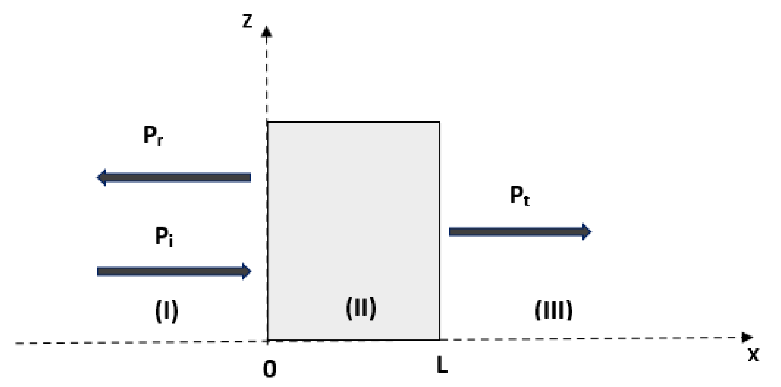
4. The Scattering Operators

In a two-dimensional problem (X-Z), a poroelastic material of thickness L, which is supposed to be homogeneous and isotropic, is saturated by a viscous fluid and found to be disturbed by a high-frequency sound wave that arrives in normal incidence on the left boundary of the material (x = 0); the geometry of the problem is represented in the Figure 1.
A part of the incident wave is reflected in the fluid and the other one is transmitted through the porous medium in the shape of the three waves of Biot: the two compressional waves and a shear wave. By pointing out the fact that the porous medium occupies the region (0 ≤ xL), we can see that the expression of the pressure field in the region (I), where x < 0 , is the sum of the incident p i and the reflected p r fields.
p 1 ( x , t ) = p i t x c 0 + p r t + x c 0 , x < 0 ,
where p 1 ( x , t ) is the total pressure field at the left of the medium. In the limit x > L , the pressure field results from the transmission of the incident wave through the porous material and is given by the following:
p 3 ( x , t ) = p t t x L c 0 , x > L ,
where p t is the pressure of the transmitted wave.
The expressions of the reflected and transmitted pressure fields can be established by integrating the product of the scattering operators (R and T) by the incident wave, which gives the following:
p r ( x , t ) = 0 t R ˜ ( τ ) p i t τ + x c 0 d τ
p t ( x , t ) = 0 t T ˜ ( τ ) p i t τ L c ( x L ) c 0 d τ .
The fact that the lower limit of the integrals of these expressions is zero indicates that it is exactly at t = 0 that the incident wavefront hits the material for the first time.
Accordingly, p 1 ( x , t ) and p 3 ( x , t ) are expressed by the following equations:
p 1 ( x , t ) = 0 t δ τ x c 0 + 0 τ R ˜ τ δ τ τ + x c 0 d τ p i ( t τ ) d τ
p 3 ( x , t ) = 0 t 0 τ T 1 ˜ τ p i ( x , τ τ ) d τ δ t τ L c 1 x L c 0 d τ + 0 t 0 τ T 2 ˜ τ p i ( x , τ τ ) d τ δ t τ L c 2 x L c 0 d τ .
T 1 t and c 1 are the transmission operator and the propagation speed of the fast wave, respectively. Similarly, T 2 t and c 2 are the transmission operator and the propagation speed of the slow wave, respectively.
To simplify the analysis, as previously achieved, we use the Laplace transform, which is more adequate for our problem. We note that, following the definition in (15), P ( x , s ) is the Laplace transform of p ( x , t ) . The pressure fields on both sides of the medium in the Laplace domain are given by the following:
P 1 ( x , s ) = ( e x c 0 s + R ( s ) e x c 0 s ) P ( s ) ,
P 3 ( x , s ) = T ( s ) P ( s ) e x L c 0 s ,
with
T ( s ) = T 1 s e L c 1 s + T 2 s e L c 2 s .
P 1 ( x , s ) and P 3 ( x , s ) are, respectively, the Laplace transform of the field at the left and right of the material; P ( s ) is the Laplace transform of the incident field; and finally, R ( s ) and T ( s ) are the Laplace transforms of the reflection and transmission operators.
The stress–strain equations in the porous medium are given by
σ i j s = P 2 N . u + Q . U δ i j + N ( u i , j + u j , i ) , σ i j f = R . U + Q . u = p f δ i j . ,
where σ i j a are the components of the stress tensor that act on the solid (a = s) or fluid (a = f) phase and ϵ i j = 1 2 ( u i j + u j i ) is the skeletal strain tensor.
Since the pressure and stress fields at the boundaries of the medium are continuous [39], the relations between the pressure field and the stresses in the Laplace domain at the interfaces x = 0 and x = L are given by the following:
σ s ( 0 + , s ) = ( 1 ϕ ) P 1 ( 0 , s ) , σ f ( 0 + , s ) = ϕ P 1 ( 0 , s ) , σ s ˜ ( 0 + , s ) = 0 σ s ( L , s ) = ( 1 ϕ ) P 3 ( L + , s ) , σ f ( L , s ) = ϕ P 3 ( L + , s ) , σ s ˜ ( L , s ) = 0
σ s and σ f are the normal stresses in the skeleton and fluid, respectively, and σ s ˜ is the shear stress in the skeleton; their expressions in the Laplace domain take the following form:
σ x x s ( x , s ) = P 2 N 2 Φ s ( x , s ) x 2 + Q 2 Φ f ( x , s ) x 2 + 2 N 2 Φ s ( x , s ) x 2 , σ x x f ( x , s ) = Q 2 Φ s ( x , s ) x 2 + R 2 Φ f ( x , s ) x 2 , σ s ˜ ( x , s ) = 2 N 2 Φ s ( x , s ) x 2 + 2 Ψ s ˜ ( x , s ) x 2 ,
where Φ s Φ f and Ψ s ˜ are the Laplace transforms of ϕ s , ϕ f , and Ψ s .
Hence, using the boundary conditions in (37), the expressions of the scalar functions Φ 11 ( s )   Φ 12 ( s ) , Φ 21 ( s ) , Φ 22 ( s ) , Ψ 1 ˜ ( s ) and Ψ 1 ˜ ( s ) are calculated in Appendix B.
To determine the reflection and transmission coefficients, we consider the conservation conditions of the flow at the limits of the medium ( x = 0 and x = L ):
V 1 ( 0 + , s ) = ( 1 ϕ ) V s ( L , s ) + ϕ V f ( L , s ) , V 3 ( L , s ) = ( 1 ϕ ) V s ( L , s ) + ϕ V f ( L , s ) .
In those expressions, V 1 ( x , s ) and V 3 ( x , s ) are, respectively, the acoustic velocity fields in the regions x < 0 and x > L , while V s ( x , s ) and V f ( x , s ) are the velocities of the solid and fluid in the porous medium, respectively.
The acoustic velocity fields are obtained by considering the field pressure of the surrounding fluid in (34) and (), and the Euler equation:
ρ f s V i ( x , s ) = P i ( x , s ) x , i = 1 , 2 , 3 .
The expressions of V s and V f are found using the following expressions:
V s ( x , s ) = s ( Φ s + Ψ s ) , V f ( x , s ) = s ( Φ f + Ψ f ) .
Using the boundary conditions in (38) and the expressions for the fluid and solid velocity fields, V s ( x , s ) ), V f ( x , s ) , V 1 ( x , s ) , and V 3 ( x , s ) , we obtain the expressions for the transmission and reflection coefficients in the Laplace domain:
R ( s ) = s 2 F 5 2 ( s ) F 4 2 ( s ) + 1 ( s F 4 ( s ) 1 ) 2 s 2 F 5 2 ( s ) ,
T ( s ) = 2 s F 5 ( s ) ( s F 4 ( s ) 1 ) 2 s 2 F 5 2 ( s ) ,
where
F 4 ( s ) = F 1 ( s ) cosh l λ 1 ( s ) + F 2 ( s ) cosh l λ 2 ( s ) + F 3 ( s ) cosh l λ 3 ( s ) , F 5 ( s ) = F 1 ( s ) + F 2 ( s ) + F 3 ( s ) , F i ( s ) = ρ f c 0 1 + ϕ ( V i ( s ) 1 ) λ 1 ( s ) 2 Ψ i " ( s ) sinh ( l λ i ( s ) ) Ψ " ( s ) , V i ( s ) = A i + B i s , i = 1 , 2 , λ i ( s ) = C i s 2 + D i s 3 2 + G i s , i = 1 , 2 V 3 ( s ) = A 3 + B 3 s , λ 3 ( s ) = C 3 s 2 + D 3 s 3 2 + G 3 s .
The coefficients Ψ 1 " ( s ) Ψ 2 " ( s ) Ψ 3 " ( s ) and Ψ " ( s ) are given by
Ψ 1 " ( s ) = ϕ Z 2 ( s ) ( 1 ϕ ) Z 4 ( s ) , Ψ 2 " ( s ) = ( 1 ϕ ) Z 3 ( s ) ϕ Z 1 ( s ) , Ψ 3 " ( s ) = ( 1 ϕ ) Z 8 ( s ) ϕ Z 9 ( s ) , Ψ " ( s ) = 2 ( Z 1 ( s ) Z 4 ( s ) Z 2 ( s ) Z 3 ( s ) ) .
The coefficients Z i ( s ) are given by
Z 1 ( s ) = ( V 1 Q + P ) λ 1 ( s ) , Z 2 ( s ) = ( V 2 Q + P ) λ 2 ( s ) , Z 3 ( s ) = ( V 1 R + Q ) λ 1 ( s ) , Z 4 = ( V 2 R + Q ) λ 2 ( s ) , Z 5 ( s ) = 2 N λ 1 ( s ) , Z 6 ( s ) = 2 N λ 2 ( s ) , Z 7 = 2 N λ 3 ( s ) , Z 8 ( s ) = Z 6 ( s ) Z 3 ( s ) Z 5 ( s ) Z 4 ( s ) Z 7 ( s ) , Z 9 ( s ) = Z 6 ( s ) Z 1 ( s ) Z 5 ( s ) Z 2 ( s ) Z 7 ( s ) .
The scattering operators are obtained in the Laplace domain. The purpose of our work is to determine these operators in the time domain, but using the inverse Laplace transform to go directly to the time domain is a very difficult task to perform because of the complexity of these operators. For this reason, modifications and simplifications are applied (Appendix A) to the relations in (40) and (), which allows us to find the time equivalent of the reflection and transmission operators:
R ( t ) = r ( t ) + R ( t ) ˜ ,
where
r ( t ) = 1 + U 1 U δ ( t ) + 2 a 1 U 1 π t + a exp ( a 2 t ) E r f c ( a t ) ,
and
R ( t ) ˜ = 4 ( 1 U ) 2 x 1 G 1 ( t , 2 L ) + x 2 G 2 ( t , 2 L ) + x 3 G 3 ( t , 2 L ) + 4 ( 1 U ) 2 P 1 ( t ) G 1 ( t , 2 L ) + P 2 ( t ) G 2 ( t , 2 L ) + P 3 ( t ) G 3 ( t , 2 L ) .
T ( t ) = 4 ( 1 U ) 2 x 1 G 1 ( t , L ) + x 2 G 2 ( t , L ) + x 3 G 3 ( t , L ) 4 ( 1 U ) 2 P 1 ( t ) G 1 ( t , L ) + P 2 ( t ) G 2 ( t , L ) + P 3 ( t ) G 3 ( t , L ) .
The expressions of P i ( t ) and G i ( t , L ) are given by
P i ( t ) = y i 2 a x π t + 2 a 2 ( y i a x i ) t π + a 2 x i ( 3 + 2 a 2 t ) 2 a y i ( 1 + a 2 t ) × exp ( a 2 t ) E r f c ( a t ) , i = 1 , 2 , 3
G i ( t , j L ) = L 1 exp j L λ 1 ( s ) , i = 1 , 2 , 3 , j = 1 , 2
G i ( t ) , i = 1 , 2 , 3 , are the Green functions of compressional (first and second species) and shear waves, respectively; they describe the propagation of each of these waves inside the porous medium, and their expressions are given in Appendix A.
G i ( t ) , i = 1 , 2 , 3 , are the Green functions of the longitudinal (fast and slow) and transverse waves, respectively. They describe the propagation of each of these waves inside the porous medium, and their expressions are given in Appendix A.
Knowing the strong attenuation that the acoustic wave undergoes in a porous media saturated by a viscous fluid makes multiple reflections negligible; thus, we take only the first reflections at the interfaces x = 0 and x = L in the expressions of the operators in (42) and (45).
The first term of the second member of Equation (43) corresponds to the instantaneous reflection of the wave by the first interface x = 0 . The reflected wave does not have time to propagate in the medium, which gives it the advantage of not being dispersive but only attenuated by the term 1 + U 1 U .
The second term of r ( t ) expresses the attenuation and dispersion process since it depends on the fractional derivative operator, which takes into account the viscousfluid–structure interaction effects during the wave propagation. This memory term expresses the phenomenon of relaxation of the wave reflected by the first interface.
The term of the second member of Equation (45) corresponds to the reflection by the second interface x = L . This term depends on the Green function of the longitudinal and transverse waves that describe the propagation and dispersion of these waves inside the porous material just as R ( t ) ˜ the temporal expression of the transmission operator in (45) depends on the Green functions of the three Biot waves, highlighting the contribution of each of these waves to the total transmitted wave.
From the temporal expressions of the scattering operators obtained in (42) and (45), the effect of the shear wave plus the effect of the compressional waves (fast and slow) on the porous medium’s response to an external load can be examined. It is also possible to study the influence of the characteristic parameters of the porous medium on the amplitudes and speed of these waves.

5. Numerical Validation

In order to test the validity of our analytical development and to show the influence that the shear waves can have on the response of bone-type porous materials, we proceed to compare transmitted signals obtained during this study, the shear waves being taken into account, and the transmitted signals, where only the longitudinal waves are observed because the shear waves are very weak in normal incidence; however, whether or not they are taken into account is visible on the longitudinal waveforms, as shown in the following study. The characteristics of the bone samples used in this study were taken from work carried out previously by Fellah [67] and are shown in Table 1.
The transmitted signals are computed by performing the convolution product of the transmission operator given by (45) with the incident signal, as in the relation in ().

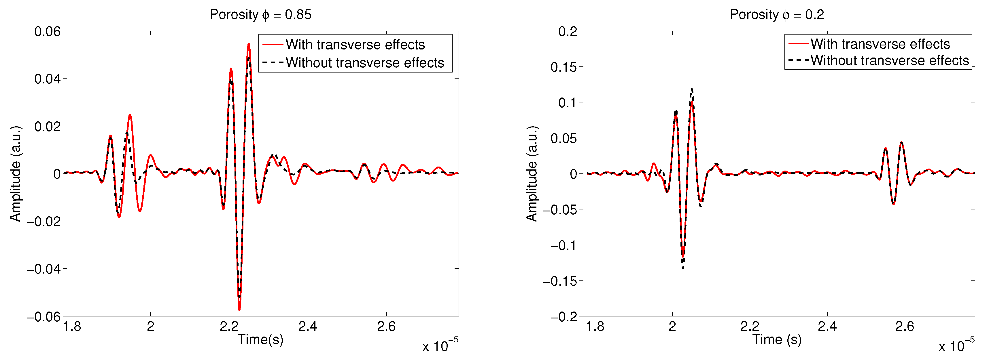
5.1. Porosity Variation

The two waves observed in the numerical simulations (Figure 2) correspond to the slow and fast longitudinal waves. The shear wave is not noticeable because of its low amplitude at normal incidence; however, its effect is visible on the velocities and amplitudes of the longitudinal waves. This is the subject of the following sensitivity study.
The transmitted signals are simulated by taking or not taking into account the transverse wave for two distinct porosities: ϕ = 0.2 and ϕ = 0.85 .  Figure 2 depicts the impact of the shear wave on different values of the porosity. When the porosity value is equal to 0.2, the shear effect is not felt in the slow longitudinal wave, and its amplitude and speed do not change, unlike the amplitude and speed of the fast wave. For the value of the porosity of 0.85, we notice that, whether the shear wave is considered is much more important than in the previous case (when the porosity was equal to 0.2) for the amplitudes of the fast and slow longitudinal waves. We can therefore conclude at this stage that the effect of shear is more visible as the value of porosity is high and at the level of the amplitudes of both longitudinal waves. The velocities of the longitudinal waves do not seem to be affected by whether or not shear is taken into account.

5.2. Tortuosity Variation

Figure 3 represents a comparison of the simulated transmitted signals when only the effect of longitudinal waves is considered (black dotted line) and when the effect of the transverse waves is combined with that of the longitudinal waves (red line) for two different values of the tortuosity α = 1 and α = 1.3 .
Readers can notice that the amplitudes of the two compressional waves (the fast and slow) are different for the two values of tortuosity, even though it is more apparent for α = 1.3 than it is for α = 1 . The velocities of both compressional waves remain unchanged, regardless of whether the effect of the transverse waves is included or not.
Tortuosity is an important parameter to describe the inertial effects, which occur between the fluid and solid parts of a porous material because it provides information on the geometry of the pores of the porous medium, which are rarely straight and have variable sections. Like porosity variations, tortuosity variations cause changes in the fast and slow waves and their velocities.
Comparing the figures for two values of the tortuosity, we notice that an increase in the tortuosity induces an increase in the amplitude of the fast wave and a decrease in the amplitude of the slow-wave. A temporal shift of the two Biot waves occurs (decrease in the velocities), which is more distinct on the slow wave than it is on the fast wave as the tortuosity increases.

5.3. Variation of the Viscous Characteristic Length
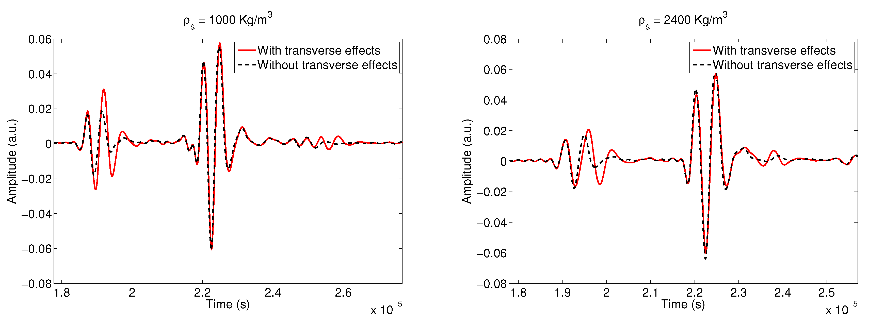
 Λ

The effect of whether transverse waves are considered along with longitudinal waves on the transmitted signals for two different viscous characteristic lengths is illustrated in Figure 4. In the comparison of the simulated transmitted signals, the effect of shear can be observed on the amplitudes of both the fast and slow waves. This effect leads to an increase in the amplitudes of the fast and slow waves regardless of the value of the viscous characteristic length. The speeds of the fast and slow waves remain unchanged in all cases. The comparison between the figures corresponding to two values of the viscous characteristic length provides information on the effect of the viscous characteristic length on the transmitted signals. This parameter was first introduced by Johnson et al. [33] in 1987 and is considered to be a geometrical parameter indicative of small pore sizes; it represents the thickness where viscous effects are important.
Through our comparison, we can see that, by increasing the viscous characteristic length from 5 μ m to 9 μ m, the amplitude of the slow wave increases while the velocities of the slow and fast waves as well as the amplitude of the fast wave remain practically the same.
The viscous characteristic length plays a less important role than the tortuosity, since the variation in its value barely affects the transmitted signals whether the shear wave is considered or not.

5.4. Solid Density ρ s Variation

The difference between the transmitted signals when shear effects are considered and not considered along with longitudinal waves for two distinct values of the solid density ρ s = 1000 kg/m 3 and ρ s = 2400 kg/m 3 is given in Figure 5. Unlike for the previous case of the effect of the viscous characteristic length, we notice that the only significant difference is for the amplitudes of the fast waves that increase when the shear waves are considered for both values of the solid density; the slow waves are practically the same for both signals in Figure 5. It is worth mentioning that, for a high value of the density ρ s = 2400 kg/m 3 , the fast wave with shear taken into account arrives faster than the one with shear not taken into account, which means that its speed is greater without than with shear taken into account, which is not observed for the slow wave.
We can also notice from these figures that the fast waves (amplitude and speed) are sensitive to the variation of the solid density; indeed, a decrease in the amplitudes of the fast waves as well as a decrease in their speed appear when the solid density goes from 1000 (kg/m 3 ) to 2400 (kg/m 3 ).

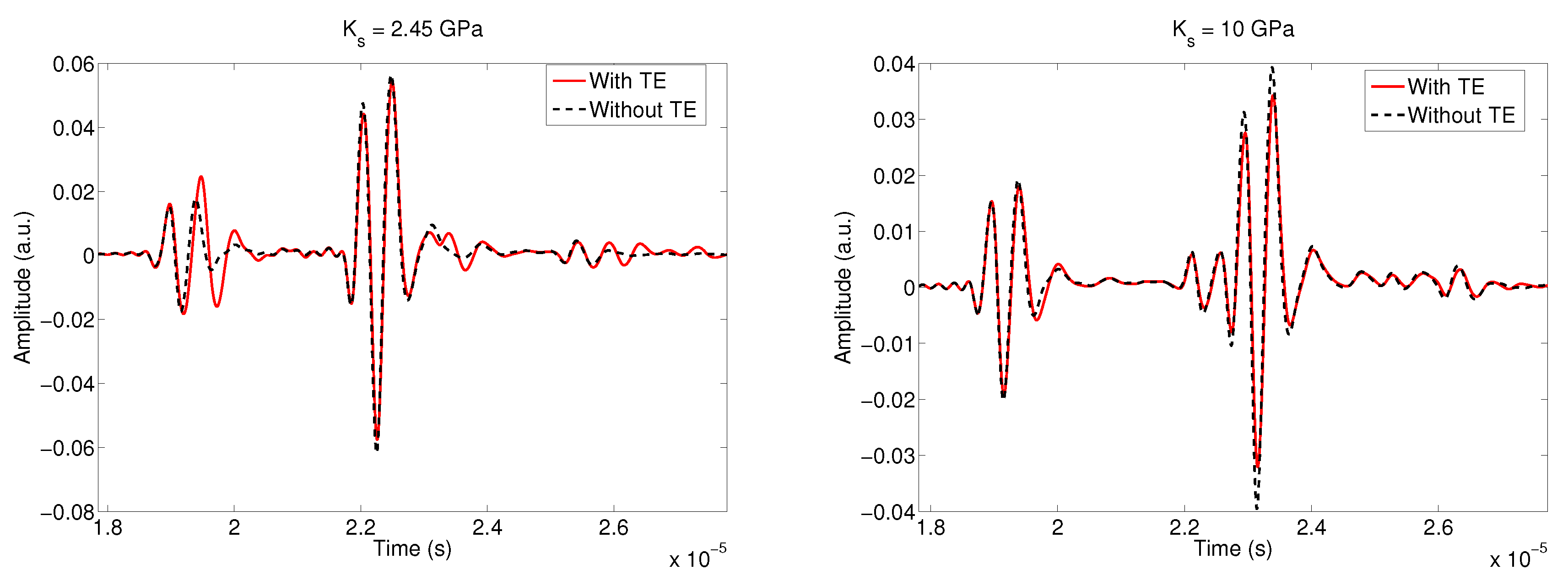
5.5. Bulk Modulus of the Elastic Solid K s Variation

The simulated transmitted signals with and without considering the effect of transverse waves in addition to longitudinal waves are compared in Figure 6 for two values of the bulk modulus of the elastic solid K s . We notice that the effect of the shear wave is visible mainly on the amplitude of the fast wave for the value of K s = 2.45 GPa, and the amplitude of the slow wave varies but in a lesser way. For the value of K s = 10 GPa, it is the amplitude of the slow wave that is most sensitive to the incorporation of shear in the model, with the change in the amplitude of the fast wave being, however, smaller for this value of K s . Shear affects the amplitudes of the fast and slow waves differently depending on the values of K s .
The speed of the fast wave also seems to be sensitive to the shear; in fact, when decreasing the value of K s , the fast wave arrives delayed when the shear is not taken into account. In other words, taking into account the shear increases the speed of the fast wave, which makes it arrive faster in comparison with the fast wave obtained without shear. This phenomenon is not observable for the speed of the fast wave when K s = 10 GPa or for the speeds of the slow waves, regardless of the value of K s .

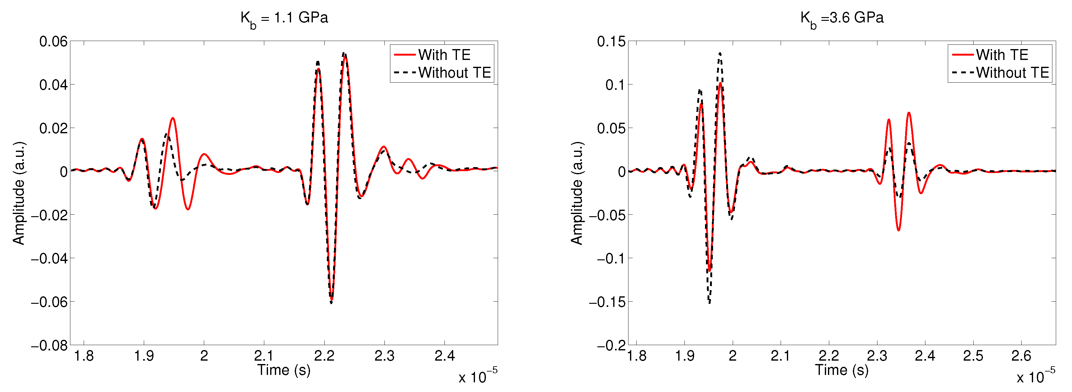
5.6. Bulk Modulus of the Porous Skeletal Frame K b Variation

The sensitivity study of the bulk modulus of the porous skeletal frame K b taking or not taking into account the shear shows quite interesting results compared with the previous cases (see Figure 7). For example, we notice as an example that, for the high value of K b = 3.6 GPa, the amplitudes of the slow and fast waves are very affected by whether shear is considered. The amplitude of the slow wave in this case can be doubled when the shear is taken into account, while the amplitude of the slow wave decreases sharply. For the value of K b = 1.1 GPa, the variation in the slow wave amplitude is very small while that of the fast wave is much larger. We also notice generally that the velocities of the waves do not practically change with the taking into account of the shear, except for that of the fast wave for K b = 1.1 GPa, where we see that taking shear into account of the shear decreases the velocity of the fast wave, which slows down compared with the case where the shear is taken into account.

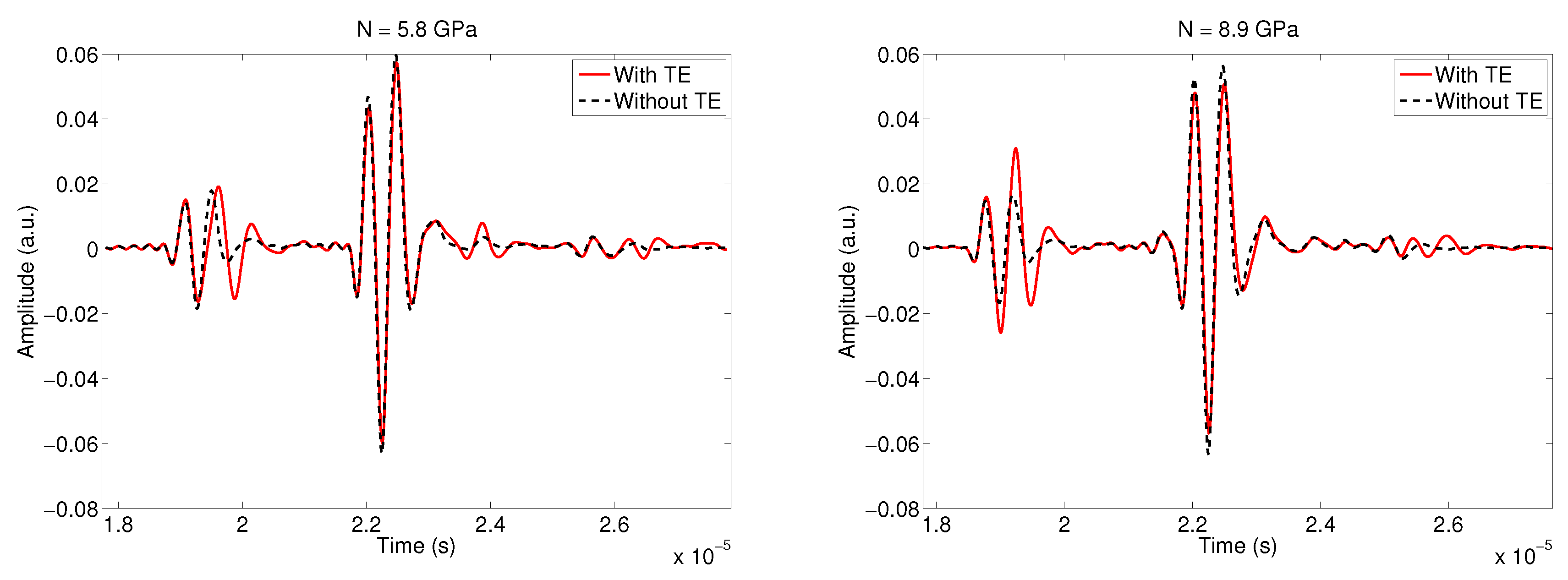
5.7. The Shear Modulus N Variation

The simulated transmitted signals including and excluding the effect of the shear wave in addition to the longitudinal waves for two values of the shear modulus are shown in Figure 8. The comparison between the two signals for each value of N allows us to say that the inclusion of the shear wave in the model affects the fast wave more than the slow wave and more particularly for large values of N ( N = 8.9 GPa). However, the effect of shear is more visible on the speed of the fast wave for low values of N ( N = 5.8 GPa). However, the slow wave velocities remain unchanged whether shear is considered or not.

6. Discussion and Conclusions

This study allows us to examine the influence of the shear wave in the modeling of ultrasound propagation in porous media. This effect is studied by comparing the transmitted waveforms by varying each physical parameter of the porous material (porosity, tortuosity, viscous characteristic length, density of the solid, bulk modulus of the elastic solid, bulk modulus of the porous skeletal frame, and shear modulus). The amplitudes and velocities of the transmitted longitudinal waves (slow and fast) are observed and compared in order to see the impact of taking into account the shear wave in the model. In our previous work [19,62], we did not take into account the shear wave at normal incidence, but recent studies [62,67] have shown that the shear wave must be taken into account because of the viscous exchanges between fluid and structure. At normal incidence, the shear wave is not as visible as the fast and slow longitudinal waves because its amplitude is very low; however, its effect is felt in the amplitudes and speeds of longitudinal waves, and this effect varies depending on the values of the physical parameters of the porous medium, as shown in this study.
The originality of our approach is that it makes it possible not only to model in the time domain acoustic propagation in a porous medium using fractional calculus but also to obtain analytical solutions to the response (reflection and transmission operators) of the porous medium to an acoustic excitation (incident wave). This analytical solution in the time domain expressed by the Green functions of longitudinal (fast and slow) and transverse waves using fractional calculation is the strong point (original) of our work. Indeed, the the existing studies do not provide analytical solutions but only propose numerical solutions.
The study of the sensitivity of the physical parameters of the longitudinal waves by taking or not taking into account the shear wave in the model allows us to see and quantify the importance of the shear wave in the modeling and its impact on the longitudinal waves. It appears that the variation in the the values of some parameters such as the bulk modulus of the porous skeletal frame reflects a significant change in the amplitude of the fast and slow longitudinal waves. The velocity of the fast wave is also modified, contrary to that of the fast wave, which is unchanged, and thus independent of whether shear is taken into account. The variation in other parameters (such as porosity, tortuosity, viscous characteristic length, solid density, and shear modulus) modifies the amplitude of the fast wave more than that of the slow wave. Practically for all the parameters, their variation has no impact on the speed of the slow wave, only on that of the fast wave.
The results of this study clearly show that the inclusion of the shear wave in the model has a considerable impact on the amplitude of the slow and fast waves as well as on the speed of the fast wave. The fractional calculus have proven to be very useful in obtaining the analytical solutions in the time domain. We can then conclude that the shear wave at normal incidence should no longer be ignored as it was the case in the previous studies and that it is necessary to consider the shear effects, as this will have consequences for the acoustic and mechanical characterization of porous materials by solving the inverse problems using experimental data of transient waves.

Author Contributions

Writing—original draft preparation, D.B. (Djihane Benmorsli), D.B. (Djema Belgroune), Z.E.A.F., M.F., E.O., N.O.O. and C.D.; analysis, analytical calculations, and processing of results, D.B. (Djihane Benmorsli), D.B. (Djema Belgroune), Z.E.A.F., M.F., E.O. and C.D.; writing—review and editing, D.B. (Djihane Benmorsli), D.B. (Djema Belgroune), Z.E.A.F., M.F., E.O. and C.D.; resources, D.B. (Djihane Benmorsli), D.B. (Djema Belgroune), Z.E.A.F., M.F., E.O. and C.D. All authors have read and agreed to the published version of the manuscript.

Funding

This research received no external funding.

Institutional Review Board Statement

Not applicable.

Informed Consent Statement

Not applicable.

Data Availability Statement

Not applicable.

Conflicts of Interest

The authors declare no conflict of interest.

Appendix A. The Eigenvalues and Eigenvectors of the Matrix M

The matrix M is given in the Laplace domain by the following:
M = ( R ρ 11 Q ρ 12 ) s 2 + A s 3 2 ( R + Q ) ( R ρ 12 Q ρ 22 ) s 2 A s 3 2 ( R + Q ) ( P ρ 12 Q ρ 11 ) s 2 A s 3 2 ( P + Q ) ( P ρ 22 Q ρ 12 ) s 2 + A s 3 2 ( P + Q ) ,
with
R Q Q P = P Q Q R 1 = R P R Q 2 Q P R Q 2 Q P R Q 2 P P R Q 2 ,
and
A = 2 ϕ α ρ f Λ η ρ f 1 2 .
The eigenvalues of the matrix M are written as follows:
λ 1 , 2 ( s ) = t r ( M ) ± t r ( M ) 2 4 det ( M ) 2 2 ,
where T r a ( M ) and D e t ( M ) are, respectively, the trace and determinant of this same matrix:
T r a ( M ) = ( R ρ 11 2 Q ρ 12 + P ρ 22 ) s 2 + A s 3 2 ( R + 2 Q + P ) , D e t ( M ) = ( P R Q 2 ) ρ 11 ρ 12 ρ 12 2 s 4 + A s 7 2 ( ρ 11 + ρ 22 2 ρ 12 ) .
Posing
τ 1 = R ρ 11 2 Q ρ 12 + P ρ 22 , τ 2 = A ( R + 2 Q + P ) , τ 3 = ( P R Q 2 ) ρ 11 ρ 12 ρ 12 2 , τ 4 = ( P R Q 2 ) ( ρ 11 + ρ 22 2 ρ 12 ) A ,
and
C i = 1 2 τ 1 + ( 1 ) i ( τ 1 2 4 τ 3 , D i = 1 2 τ 2 + ( 1 ) i τ 1 τ 2 2 τ 4 ( τ 1 2 4 τ 3 , G i = ( 1 ) i 1 4 τ 2 2 ( τ 1 2 4 τ 3 ( τ 1 τ 2 2 τ 4 ) 2 2 ( τ 1 2 4 τ 3 ) 3 2 ,
we obtain the expressions of the eigenvalues:
λ i ( s ) = C i s 2 + D i s 3 2 + G i s , i = 1 , 2 .
The expressions of the components V 1 , 2 of the eigenvectors are given by
V 1 , 2 ( s ) = λ 1 , 2 ( s ) ( R ρ 11 Q ρ 12 ) s 2 + A s 3 2 ( R + Q ) ( R ρ 12 Q ρ 22 ) s 2 A s 3 2 ( R + Q ) .
By posing
τ 5 = ( R ρ 11 Q ρ 12 ) , τ 6 = A ( R + Q ) , τ 7 = ( R ρ 12 Q ρ 22 ) ,
A i = τ 1 2 τ 5 + ( 1 ) i ( τ 1 2 4 τ 3 2 τ 7 , B i = 1 4 τ 7 2 τ 2 2 τ 6 + ( 1 ) i ( τ 1 τ 2 2 τ 4 ) ( τ 1 2 4 τ 3 ) 3 2 2 τ 7 + τ 1 2 τ 5 ( τ 1 2 4 τ 3 ) 1 2 2 τ 6 , i = 1 , 2
we obtain
V i ( s ) = A i + B i s , i = 1 , 2 .

Appendix B. Scalar Functions

The components of the stress tensor σ i j s that act on the solid ( a = s ) or fluid ( a = f ) phase are given by
σ i j s = P 2 N . u + Q . U δ i j + N ( u i , j + u j , i ) , σ i j f = R . U + Q . u = p f δ i j .
The stress–strain relationship for the fluid in the Laplace domain is in the following form:
σ ˜ x x f ( x , s ) = R . U + Q . u ,
with
u ( x , s ) = Φ s ( x , s ) , U ( x , s ) = Φ f ( x , s ) ,
σ x x f ( x , s ) = R 2 Φ s ( x , s ) x 2 + Q 2 Φ f ( x , s ) x 2 ,
where
Φ s ( x , s ) = Φ 1 ( x , s ) + Φ 2 ( x , s ) , Φ f ( x , s ) = V 1 ( s ) Φ 1 ( x , s ) + V 2 ( s ) Φ 2 ( x , s ) ,
and we find
σ x x f ( x , s ) = ( V 1 ( s ) R + Q ) 2 Φ 1 ( x , s ) x 2 + ( V 2 ( s ) R + Q ) 2 Φ 2 ( x , s ) x 2 .
By replacing Φ 1 ( x , s ) and Φ 2 ( x , s ) by their expressions in (19) and (20), we find
σ x x f ( x , s ) = Z 3 ( s ) ( Φ 11 + Φ 12 ) cosh ( x λ 1 ( s ) ) Z 3 ( Φ 11 Φ 12 ) sinh ( x λ 1 ) + Z 4 ( Φ 21 + Φ 22 ) cosh ( x λ 2 ) Z 4 ( Φ 21 Φ 22 ) sinh ( x λ 2 )
with:
Z 3 ( s ) = ( V 1 R + Q ) λ 1 ( s ) , Z 4 ( s ) = ( V 2 R + Q ) λ 2 ( s ) ,
The stress–strain relation for the solid in the Laplace domain is in the following form:
σ x x s ( x , s ) = P 2 N . u ( x , s ) + Q . U ( x , s ) + 2 N u ( x , s ) x ,
where the solid displacement vectors are given by
u ( x , s ) = Φ s ( x , s ) , U ( x , s ) = Φ f ( x , s ) .
The normal component of the stress tensor acting on the solid part becomes the following:
σ x x s ( x , s ) = P 2 N . u ( x , s ) + Q . U ( x , s ) + 2 N u ( x , s ) x , σ x x s ( x , s ) = P 2 Φ s ( x , s ) x 2 + Q 2 Φ f ( x , s ) x 2 .
Considering the expressions for Φ 1 ( x , s ) and Φ 2 ( x , s ) , we obtain the following:
σ x x s ( x , s ) = Z 1 ( s ) ( Φ 11 + Φ 12 ) cosh ( x λ 1 ( s ) ) Z 1 ( s ) ( Φ 11 Φ 12 ) sinh ( x λ 1 ( s ) ) + Z 2 ( s ) ( Φ 21 + Φ 22 ) cosh ( x λ 2 ( s ) ) Z 2 ( s ) ( Φ 21 Φ 22 ) sinh ( x λ 2 ( s ) ) ,
with
Z 1 ( s ) = ( V 1 ( s ) Q + P ) λ 1 ( s ) , Z 2 ( s ) = ( V 2 ( s ) Q + P ) λ 2 ( s ) .
For shear wave, the stress–strain relationship is written as follows:
σ s ˜ ( x , s ) = N ( u i , j + u j , i ) σ s ˜ ( x , s ) = 2 N u ( x , s ) x ,
Using the fact that the displacement vector of the solid is
u = Φ s + Ψ s ,
the shear stress becomes
τ x x ( x , s ) = Z 5 ( s ) ( Φ 11 + Φ 12 ) cosh ( x λ 1 ( s ) ) Z 5 ( s ) ( Φ 11 Φ 12 ) sinh ( x λ 1 ) + Z 6 ( s ) ( Φ 21 + Φ 22 ) cosh ( x λ 2 ( s ) ) Z 6 ( s ) ( Φ 21 Φ 22 ) sinh ( x λ 2 ( s ) ) + Z 7 ( s ) ( Ψ 1 + Ψ 2 ) cosh ( x χ ( s ) ) Z 7 ( s ) ( Ψ 1 Ψ 2 ) sinh ( x χ ( s ) ) ,
with
Z 5 = 2 N λ 1 , Z 6 = 2 N λ 2 , Z 6 = 2 N χ .
The continuity conditions for solid and fluid stresses at x = 0 and x = L are as follows:
σ x x s ( 0 + , s ) = ( 1 ϕ ) P 1 ( 0 , s ) , σ x x f ( 0 + , s ) = ϕ P 1 ( 0 , s ) , τ x x ( 0 + , s ) = 0 .
σ x x s ( L , s ) = ( 1 ϕ ) P 3 ( L + , s ) , σ x x f ( L , s ) = ϕ P 3 ( L + , s ) , τ x x ( L , s ) = 0 .
By using the expressions of the constraints and those of the pressure fields in (34) and (), we obtain
Φ 11 ( s ) = P ( s ) Ψ 1 " Ψ " ( 1 + R ( s ) 1 + cosh ( l λ 1 ( s ) ) sinh ( l λ 1 ( s ) ) T ( s ) sinh ( l λ 1 ( s ) ) , Φ 12 ( s ) = P ( s ) Ψ 1 " Ψ " ( 1 + R ( s ) 1 cosh ( l λ 1 ( s ) ) sinh ( l λ 1 ( s ) ) + T ( s ) sinh ( l λ 1 ( s ) ) , Φ 21 ( s ) = P ( s ) Ψ 2 " Ψ " ( 1 + R ( s ) 1 + cosh ( l λ 2 ( s ) ) sinh ( l λ 2 ( s ) ) T ( s ) sinh ( l λ 2 ( s ) ) , Φ 11 ( s ) = P ( s ) Ψ 2 " Ψ " ( 1 + R ( s ) 1 cosh ( l λ 2 ( s ) ) sinh ( l λ 2 ( s ) ) + T ( s ) sinh ( l λ 2 ( s ) ) , Ψ 1 ( s ) = P ( s ) Ψ 3 " Ψ " ( 1 + R ( s ) 1 + cosh ( l χ ( s ) ) sinh ( l χ ( s ) ) T ( s ) sinh ( l χ ( s ) ) , Ψ 2 ( s ) = P ( s ) Ψ 3 " Ψ " ( 1 + R ( s ) 1 cosh ( l χ ( s ) ) sinh ( l χ ( s ) ) + T ( s ) sinh ( l χ ( s ) ) ,
with
Ψ 1 " ( s ) = ϕ Z 2 ( s ) ( 1 ϕ ) Z 4 ( s ) , Ψ 2 " ( s ) = ( 1 ϕ ) Z 3 ( s ) ϕ Z 1 ( s ) , Ψ 3 " ( s ) = ( 1 ϕ ) Z 8 ( s ) ϕ Z 9 ( s ) , Z 8 ( s ) = Z 5 ( s ) Z 4 ( s ) Z 6 ( s ) Z 3 ( s ) Z 7 ( s ) , Z 8 ( s ) = Z 6 ( s ) Z 1 ( s ) Z 5 ( s ) Z 2 ( s ) Z 7 ( s ) , Ψ " ( s ) = 2 ( Z 1 ( s ) Z 4 ( s ) Z 2 ( s ) Z 3 ( s ) ) .

Appendix C. The Scattering Operators in the Time Domain

The expressions for the scattering operators in the Laplace domain are given by the following:
R ( s ) = s 2 F 5 2 ( s ) F 4 2 ( s ) + 1 ( s F 4 ( s ) 1 ) 2 s 2 F 5 2 ( s ) ,
T ( s ) = 2 s F 5 ( s ) ( s F 4 ( s ) 1 ) 2 s 2 F 5 2 ( s ) .
These expressions can be decomposed into simple elements:
R ( s ) = 1 + 1 1 s ( F 4 ( s ) F 5 ( s ) + 1 1 s ( F 4 ( s ) + F 5 ( s ) ,
T ( s ) = 1 1 s ( F 4 ( s ) F 5 ( s ) 1 1 s ( F 4 ( s ) + F 5 ( s ) .
Using the expressions of F 4 ( s ) and F 5 ( s ) given by (42), the calculus of ( F 4 ( s ) + F 5 ( s ) ) as well as that of ( F 4 ( s ) F 5 ( s ) ) gives the following:
F 4 ( s ) + F 5 ( s ) = 2 ρ f c 0 1 + ϕ ( V 1 ( s ) 1 ) λ 1 ( s ) Ψ 1 " ( s ) Ψ " ( s ) coth l 2 λ 1 ( s ) + 1 + ϕ ( V 2 ( s ) 1 ) λ 2 ( s ) Ψ 2 " ( s ) Ψ " ( s ) coth l 2 λ 2 ( s ) + 1 + ϕ ( V 3 ( s ) 1 ) λ 3 ( s ) Ψ 3 " ( s ) Ψ " ( s ) coth l 2 λ 3 ( s ) ,
F 4 ( s ) F 5 ( s ) = 2 ρ f c 0 1 + ϕ ( V 1 ( s ) 1 ) λ 1 ( s ) Ψ 1 " ( s ) Ψ " ( s ) tanh l 2 λ 1 ( s ) + 1 + ϕ ( V 2 ( s ) 1 ) λ 2 ( s ) Ψ 2 " ( s ) Ψ " ( s ) tanh l 2 λ 2 ( s ) + 1 + ϕ ( V 3 ( s ) 1 ) λ 3 ( s ) Ψ 3 " ( s ) Ψ " ( s ) tanh l 2 λ 3 ( s ) .
Posing
X ( s ) = 2 ρ f c 0 1 + ϕ ( V 1 ( s ) 1 ) λ 1 ( s ) Ψ 1 " ( s ) Ψ " ( s ) , Y ( s ) = 2 ρ f c 0 1 + ϕ ( V 2 ( s ) 1 ) λ 2 ( s ) Ψ 2 " ( s ) Ψ " ( s ) , Z ( s ) = 2 ρ f c 0 1 + ϕ ( V 3 ( s ) 1 ) λ 3 ( s ) Ψ 3 " ( s ) Ψ " ( s ) ,
and
tanh l 2 λ i ( s ) = 1 2 e l λ i ( s ) 1 + e l λ i ( s ) , coth l 2 λ i ( s ) = 1 + 2 e l λ i ( s ) 1 e l λ i ( s ) ,
we obtain
R ( s ) = 1 + 1 1 X ( s ) Y ( s ) Z ( s ) + 2 X ( s ) W 1 ( s ) 1 + W 1 ( s ) + 2 Y ( s ) W 2 ( s ) 1 + W 2 ( s ) + 2 Z ( s ) W 3 ( s ) 1 + W 3 ( s ) + 1 1 X ( s ) Y ( s ) Z ( s ) 2 X ( s ) W 1 ( s ) 1 W 1 ( s ) 2 Y ( s ) W 2 ( s ) 1 W 2 ( s ) 2 Z ( s ) W 3 ( s ) 1 W 3 ( s ) .
T ( s ) = 1 1 X ( s ) Y ( s ) Z ( s ) + 2 X ( s ) W 1 ( s ) 1 + W 1 ( s ) + 2 Y ( s ) W 2 ( s ) 1 + W 2 ( s ) + 2 Z ( s ) W 3 ( s ) 1 + W 3 ( s ) 1 1 X ( s ) Y ( s ) Z ( s ) 2 X ( s ) W 1 ( s ) 1 W 1 ( s ) 2 Y ( s ) W 2 ( s ) 1 W 2 ( s ) 2 Z ( s ) W 3 ( s ) 1 W 3 ( s ) .
where
W i ( s ) = e l λ i ( s ) , i = 1 , 2 , 3 .
e l λ i ( s ) are assumed to be very small for large values of s because of the high-frequency condition assumed in our study, which allows us to use the following development:
R ( s ) = 1 + 1 1 X ( s ) Y ( s ) Z ( s ) n 0 2 n 1 X ( s ) Y ( s ) Z ( s ) n X ( s ) W 1 ( s ) 1 W 1 ( s ) + Y ( s ) W 2 ( s ) 1 W 2 ( s ) + Z ( s ) W 3 ( s ) 1 W 3 ( s ) n + 1 n X ( s ) W 1 ( s ) 1 + W 1 ( s ) + Y ( s ) W 2 ( s ) 1 + W 2 ( s ) + Z ( s ) W 3 ( s ) 1 + W 3 ( s ) n , T ( s ) = 1 1 X ( s ) Y ( s ) Z ( s ) n 0 2 n 1 X ( s ) Y ( s ) Z ( s ) n X ( s ) W 1 ( s ) 1 W 1 ( s ) + Y ( s ) W 2 ( s ) 1 W 2 ( s ) + Z ( s ) W 3 ( s ) 1 W 3 ( s ) n + 1 n X ( s ) W 1 ( s ) 1 + W 1 ( s ) + Y ( s ) W 2 ( s ) 1 + W 2 ( s ) + Z ( s ) W 3 ( s ) 1 + W 3 ( s ) n .
By considering only the small powers of W i ( s ) ,we obtain the following approximations:
R ( s ) = 1 + 2 ( 1 X ( s ) Y ( s ) Z ( s ) ) + 4 X ( s ) W 1 2 ( s ) ( 1 X ( s ) Y ( s ) Z ( s ) ) 2 1 W 1 2 ( s ) + 4 Y ( s ) W 2 2 ( s ) ( 1 X ( s ) Y ( s ) Z ( s ) ) 2 1 W 2 2 ( s ) + 4 Z ( s ) W 3 2 ( s ) 1 X ( s ) Y ( s ) Z ( s ) 2 1 W 3 2 ( s ) . T ( s ) = 4 X ( s ) W 1 ( s ) 1 X ( s ) Y ( s ) Z ( s ) 2 1 W 1 2 ( s ) 4 Y ( s ) W 2 ( s ) 1 X ( s ) Y ( s ) Z ( s ) 2 1 W 2 2 ( s ) 4 Z ( s ) W 3 ( s ) 1 X ( s ) Y ( s ) Z ( s ) 2 1 W 3 2 ( s ) .
For large values of s, we obtain the expressions of the reflection and transmission operators in the Laplace domain:
R ( s ) = 1 + 2 ( 1 X ( s ) Y ( s ) Z ( s ) ) + 4 X ( s ) W 1 2 ( s ) ( 1 X ( s ) Y ( s ) Z ( s ) ) 2 + 4 Y ( s ) W 2 2 ( s ) ( 1 X ( s ) Y ( s ) Z ( s ) ) 2 + 4 Z ( s ) W 3 2 ( s ) 1 X ( s ) Y ( s ) Z ( s ) 2 . T ( s ) = 4 X ( s ) W 1 ( s ) ( 1 X ( s ) Y ( s ) Z ( s ) ) 2 4 Y ( s ) W 2 ( s ) ( 1 X ( s ) Y ( s ) Z ( s ) ) 2 4 Z ( s ) W 3 ( s ) 1 X ( s ) Y ( s ) Z ( s ) 2 .
To obtain the Laplace inverse transform for these operators, it would be easier to explicitly define X ( s ) , Y ( s ) and Z ( s ) . Knowing that
λ 1 ( s ) Ψ 1 " ( s ) Ψ " ( s ) = ϕ ( P + Q ) Q + V 2 s ( ϕ ( P + Q ) R ) 2 Q 2 P R ( V 1 s V 2 s ) 1 λ 1 ( s ) , λ 2 ( s ) Ψ 2 " ( s ) Ψ " ( s ) = ϕ ( P + Q ) Q + V 1 s ( ϕ ( P + Q ) R ) 2 Q 2 P R ( V 2 s V 1 s ) 1 λ 2 ( s ) , λ 3 ( s ) Ψ 3 " ( s ) Ψ " ( s ) = ϕ ( P + Q ) R 2 Q 2 P R 1 λ 3 ( s ) ,
we find
X ( s ) ρ f c 0 = 1 + ϕ ( V 1 s 1 ) ϕ ( P + Q ) Q + V 2 s ( ϕ ( P + Q ) R ) Q 2 P R ( V 1 s V 2 s ) s λ 1 ( s ) .
By replacing V i s with their expressions,
X ( s ) ρ f c 0 = 1 + ϕ ( A 1 1 ) + ϕ B 1 s ϕ ( P + Q ) Q + A 2 ( ϕ ( P + Q ) R ) + B 1 s ϕ ( P + Q ) R Q 2 P R ( A 1 A 2 + B 1 B 2 s ) s λ 1 ( s ) .
Using the high-frequency approximation,
s λ 1 ( s ) = 1 C 1 1 1 2 D 1 C 1 1 s ,
we obtain
X ( s ) ρ f c 0 = 1 C 1 Q 2 P R ( A 1 A 2 ) α 1 γ 2 + 1 s ϕ γ 2 B 1 + α 1 β 2 α 1 γ 2 B 1 B 2 A 1 A 2 + 1 2 D 1 C 1 .
The same steps for Y ( s ) and Z ( s ) lead us to the following relations,
Y ( s ) ρ f c 0 = 1 C 2 Q 2 P R ( A 1 A 2 ) α 2 γ 1 + 1 s ϕ γ 2 B 2 + α 2 β 1 α 2 γ 1 B 2 B 1 A 2 A 1 + 1 2 D 2 C 2 , Z ( s ) ρ f c 0 = 1 C 3 Q 2 P R α 3 β 3 + 1 s B 3 β 3 ϕ 1 2 D 3 C 3 α 3 β 3 ,
with the following notations:
α 1 = 1 + ϕ ( A 1 1 ) , α 2 = 1 + ϕ ( A 2 1 ) , α 3 = 1 + ϕ ( A 3 1 ) , β 1 = B 1 ϕ ( P + Q ) R , β 2 = B 2 ϕ ( P + Q ) R , β 3 = ϕ ( Q + R ) R , γ 1 = ϕ ( P + Q ) Q + A 1 ( ϕ ( P + Q ) R ) , γ 2 = ϕ ( P + Q ) Q + A 2 ( ϕ ( P + Q ) R ) ,
and by posing
X = x 1 + y 1 s , Y = x 2 + y 2 s , Z = x 3 + y 3 s ,
where
x 1 = α 1 γ 2 ρ f c 0 C 1 Q 2 P R ( A 1 A 2 ) , x 1 = α 2 γ 1 ρ f c 0 C 2 Q 2 P R ( A 1 A 2 ) , x 3 = α 3 β 3 ρ f c 0 C 3 Q 2 P R , y 1 = ρ f c 0 C 1 Q 2 P R ( A 1 A 2 ) ϕ γ 2 B 2 + α 2 β 1 α 2 γ 1 B 2 B 1 A 2 A 1 + 1 2 D 2 C 2 , y 2 = ρ f c 0 C 2 Q 2 P R ( A 1 A 2 ) ϕ γ 2 B 2 + α 2 β 1 α 2 γ 1 B 2 B 1 A 2 A 1 + 1 2 D 2 C 2 , y 3 = ρ f c 0 C 3 Q 2 P R B 3 β 3 ϕ 1 2 D 3 C 3 α 3 β 3 .
Then, by putting
U = x 1 + x 2 + x 3 , V = y 1 + y 2 + y 3 ,
we obtain
1 1 X Y Z = 1 1 U V s = 1 1 U 1 a s + a ,
with
a = V ( U 1 ) .
This gives us
X ( s ) ( 1 X ( s ) Y ( s ) Z ( s ) ) 2 = 1 ( 1 U ) 2 x 1 2 a x 1 s + a + a 2 x 1 ( s + a ) 2 + y 1 s 2 a y 1 s ( s + a ) + a 2 y 1 s ( s + a ) 2
Y ( s ) ( 1 X ( s ) Y ( s ) Z ( s ) ) 2 = 1 ( 1 U ) 2 x 2 2 a x 1 s + a + a 2 x 2 ( s + a ) 2 + y 2 s 2 a y 2 s ( s + a ) + a 2 y 2 s ( s + a ) 2
Z ( s ) ( 1 X ( s ) Y ( s ) Z ( s ) ) 2 = 1 ( 1 U ) 2 x 3 2 a x 3 s + a + a 2 x 3 ( s + a ) 2 + y 3 s 2 a y 3 s ( s + a ) + a 2 y 3 s ( s + a ) 2 .
Using the inverse Laplace transforms,
L 1 1 s + a = 1 π t a exp ( a 2 t ) E r f c ( a t ) , L 1 1 ( s + a ) 2 = 2 a t π + ( 1 + 2 a 2 t ) exp ( a 2 t ) E r f c ( a t ) , L 1 1 s = 1 π t , L 1 1 s ( s + a ) = exp ( a 2 t ) E r f c ( a t ) , L 1 1 s ( s + a ) 2 = 2 a t π 2 a t exp ( a 2 t ) E r f c ( a t ) ,
we find the reflection and transmission operators in the time domain:
R ( t ) = r ( t ) + R ( t ) , ˜
where
r ( t ) = 1 + U 1 U δ ( t ) + 2 a 1 U 1 π t + a exp ( a 2 t ) E r f c ( a t ) ,
and
R ( t ) ˜ = 4 ( 1 U ) 2 x 1 G 1 ( t , 2 L ) + x 2 G 2 ( t , 2 L ) + x 3 G 3 ( t , 2 L ) + 4 ( 1 U ) 2 P 1 ( t ) G 1 ( t , 2 L ) + P 2 ( t ) G 2 ( t , 2 L ) + P 3 ( t ) G 3 ( t , 2 L ) .
T ( t ) = 4 ( 1 U ) 2 x 1 G 1 ( t , L ) + x 2 G 2 ( t , L ) + x 3 G 3 ( t , L ) 4 ( 1 U ) 2 P 1 ( t ) G 1 ( t , L ) + P 2 ( t ) G 2 ( t , L ) + P 3 ( t ) G 3 ( t , L ) ,
with
P i ( t ) = y i 2 a x π t + 2 a 2 ( y i a x i ) t π + a 2 x i ( 3 + 2 a 2 t ) 2 a y i ( 1 + a 2 t ) exp ( a 2 t ) E r f c ( a t ) , i = 1 , 2 , 3 ,
and
G i ( t , L ) = L 1 exp j L λ 1 ( s ) , i = 1 , 2 , 3 , j = 1 , 2 .

Appendix D. Green Functions of Longitudinal and Transverse Waves

The following relations are used for the Green functions G i ( t , K ) of the porous material for the fast wave i = 1 , the slow i = 2 , and the rotational i = 3 waves.
e K λ i ( s ) = e C i k s 2 + b i s s + e i s
b i = D i C i , e i = G i C i , i = ( b i 2 4 e i )
G i ( t , K ) = L 1 ( e K λ i ( z ) ) = 0 if 0 t K c i = Ξ i ( t ) + i 0 t k c i h i ( t , ζ ) d ζ if t K c i , i = 1 , 2 , 3 with
Ξ i ( t ) = b i 4 π K C i ( t K C i ) 2 / 3 exp b i 2 K 2 C i 16 ( t K C i ,
where h i τ , ζ has the following form,
h i τ , ζ = 1 4 π 3 / 2 1 τ ζ 2 K 2 c i 1 ζ 3 / 2 1 1 exp X i μ , τ , ζ 2 × X i μ , τ , ζ 1 × μ d μ 1 μ 2 a
and where
X i μ , τ , ζ = i μ τ ζ 2 K 2 C i + b i τ ζ 2 2 / 8 ζ .

References

  1. Osterhoff, G.; Morgan, E.F.; Shefelbine, S.J.; Karim, L.; McNamara, L.M.; Augat, P. Bone mechanical properties and changes with osteoporosis. Injury 2016, 47, S11–S20. [Google Scholar] [CrossRef]
  2. Cummings, S.R.; Browner, W.; Black, D.M.; Nevitt, M.C.; Browner, W.; Genant, H.K.; Cauley, J.; Ensrud, K.; Scott, J.; Vogt, T.M. Bone density at various sites for prediction of hip fractures. Lancet 1993, 341, 72–75. [Google Scholar] [CrossRef]
  3. Hui, S.L.; Slemenda, C.W.; Johnston, C. Baseline Measurement of Bone Mass Predicts Fracture in White Women. Ann. Intern. Med. 1989, 111, 355–361. [Google Scholar] [CrossRef] [PubMed]
  4. Stegman, M.; Recker, R.R.; Davies, K.; Ryan, R.; Heaney, R. Fracture risk as determined by prospective and retrospective study designs. Osteoporos. Int. 1992, 2, 290–297. [Google Scholar] [CrossRef]
  5. Wang, E.; Carcione, J.M.; Cavallini, F. Generalized Thermo-poroelasticity Equations and Wave Simulation. Surv. Geophys. 2021, 42, 133–157. [Google Scholar] [CrossRef]
  6. Abbas, I.; Hobiny, A. The thermomechanical response of a poroelastic medium with two thermal relaxation times. Multidiscip. Model. Mater. Struct. 2021, 17, 493–506. [Google Scholar] [CrossRef]
  7. Saeed, T.; Abbas, I.; Marin, M. A GL Model on Thermo-Elastic Interaction in a Poroelastic Material Using Finite Element Method. Symmetry 2020, 12, 488. [Google Scholar] [CrossRef]
  8. Saeed, T. A Study on Thermoelastic Interaction in a Poroelastic Medium with and without Energy Dissipation. Mathematics 2020, 8, 1286. [Google Scholar] [CrossRef]
  9. Alzahrani, F.; Abbas, I.A. Generalized Thermoelastic Interactions in a Poroelastic Material Without Energy Dissipations. Int. J. Thermophys. 2020, 41, 95. [Google Scholar] [CrossRef]
  10. Yousefian, O.; White, R.D.; Karbalaeisadegh, Y.; Banks, H.T.; Muller, M. The effect of pore size and density on ultrasonic attenuation in porous structures with mono-disperse random pore distribution: A two dimensional in-silico Study. J. Acoust. Soc. Am. 2018, 144, 709–719. [Google Scholar] [CrossRef]
  11. Fry, F.J.; Barger, J.E. Acoustical properties of the humain skull. J. Acoust. Soc. Am. 1978, 63, 1576–1590. [Google Scholar] [CrossRef]
  12. Ashman, R.B.; Corin, J.D.; Turner, C.H. Elastic properties of cancellous bone: Measurement by an ultrasonic technique. J. Biomech. 1987, 20, 979–989. [Google Scholar] [CrossRef]
  13. Ashman, R.B.; Rho, J.Y. Elastic modulus of trabecular bone material. J. Biomech. 1988, 21, 177–181. [Google Scholar] [CrossRef]
  14. Hosokawa, A.; Otani, T. Ultrasonic wave propagation in bovine cancellous bone. J. Acoust. Soc. Am. 1997, 101, 558–562. [Google Scholar] [CrossRef]
  15. Hosokawa, A.; Otani, T. Acoustic anisotropy in bovine cancellous bone. J. Acoust. Soc. Am. 1998, 103, 2718–2722. [Google Scholar] [CrossRef]
  16. Haire, T.J.; Langton, C.M. Biot theory: A review of its application on ultrasound propagation through cancellous bone. Bone 1999, 24, 291–295. [Google Scholar] [CrossRef]
  17. Cardoso, L.; Teboul, F.; Sedel, L.; Meunier, A.; Oddou, C. In vitro acoustic waves propagation in human and bovine cancellous bone. J. Bone Miner. Res. 2003, 18, 1803–1812. [Google Scholar] [CrossRef]
  18. Cardoso, L.; Cowin, S.C. Fabric dependence of quasi-waves in anisotropic porous media. J. Acoust. Soc. Am. 2011, 129, 3302–3316. [Google Scholar] [CrossRef]
  19. Fellah, Z.E.A.; Chapelon, J.Y.; Berger, S.; Lauriks, W.; Depollier, C. Ultrasonic wave propagation in human cancellous bone: Application of Biot theory. J. Acoust. Soc. Am. 2004, 116, 61–73. [Google Scholar] [CrossRef]
  20. Sebaa, N.; Fellah, Z.E.A.; Fellah, M.; Ogam, E.; Wirgin, A.; Mitri, F.G.; Depollier, C.; Lauriks, W. Ultrasonic characterization of human cancellous bone using the Biot theory: Inverse problem. J. Acoust. Soc. Am. 2006, 120, 1816–1824. [Google Scholar] [CrossRef]
  21. Marutyan, K.R.; Holland, M.R.; Miller, J.G. Anomalous negative dispersion in bone can result from the interference of fast and slow waves. J. Acoust. Soc. Am. 2006, 120, EL55–EL61. [Google Scholar] [CrossRef]
  22. Hughes, E.R.; Leighton, T.G.; White, P.R.; Petley, G.W. Investigation of an anisotropic tortuosity in a Biot model of ultrasonic propagation in cancellous bone. J. Acoust. Soc. Am. 2006, 121, 568–574. [Google Scholar] [CrossRef]
  23. Pakula, M.; Padilla, F.; Laugier, P.; Kaczmarek, M. Application of Biot’s theory to ultrasonic characterization of human cancellous bones: Determination of structural, material, and mechanical properties. J. Acoust. Soc. Am. 2008, 123, 2415–2423. [Google Scholar] [CrossRef]
  24. Anderson, C.C.; Marutyan, K.R.; Holland, M.R.; Wear, K.A.; Miller, J.G. Interference between wave modes may contribute to the apparent negative dispersion observed in cancellous bone. J. Acoust. Soc. Am. 2008, 124, 1781–1789. [Google Scholar] [CrossRef]
  25. Mizuno, K.; Matsukawa, M.; Otani, T.; Laugier, P.; Padilla, F. Propagation of two longitudinal waves in human cancellous bone: An in vitro study. J. Acoust. Soc. Am. 2009, 125, 3460–3466. [Google Scholar] [CrossRef]
  26. Wear, K.A. Cancellous bone analysis with modified least squares Prony’s method and chirp filter: Phantom experiments and simulation. J. Acoust. Soc. Am. 2010, 128, 2191–2203. [Google Scholar] [CrossRef]
  27. Nelson, A.M.; Hoffman, J.J.; Anderson, C.C.; Holland, M.R.; Nagatani, Y.; Mizuno, K.; Matsukawa, M.; Miller, J.G. Determination attenuation properties of interfering fast and slow ultrasonic waves in cancellous bone. J. Acoust. Soc. Am. 2011, 130, 2233–2239. [Google Scholar] [CrossRef]
  28. McKelvie, M.L. Ultrasonic Propagation in Cancellous Bone. Ph.D. Thesis, University of Hull, Hull, UK, 1988. [Google Scholar]
  29. Williams, J.L. Ultrasonic wave propagation in cancellous bone and cortical bone: Prediction of some experimental results by Biot’s theory. J. Acoust. Soc. Am. 1992, 91, 1106–1112. [Google Scholar] [CrossRef]
  30. Lauriks, W.; Thoen, J.; Asbroeck, I.V.; Lowet, G.; Vanderperre, G. Propagation of ultrasonic pulses through trabecular bone. J. Phys. Paris Colloq. 1994, 4, 1255–1258. [Google Scholar] [CrossRef]
  31. Mckelvie, M.L.; Palmer, S.B. The interaction of ultrasound with cancellous bone. Phys. Med. Biol. 1991, 10, 1331–1340. [Google Scholar] [CrossRef] [PubMed]
  32. Lakes, R.; Yoon, H.S.; Katz, J.L. Slow compressional wave propagation in wet human and bovine cortical bone. Science 1983, 220, 513–515. [Google Scholar] [CrossRef] [PubMed]
  33. Johnson, D.L.; Koplik, J.; Dashen, R. Theory of dynamic permeability and tortuosity in fluid-saturated porous media. J. Fluid Mech. 1987, 176, 379–402. [Google Scholar] [CrossRef]
  34. Buchanan, J.L.; Gilbert, R.P.; Ou, M.J. Transfer functions for a onedimensional fluid-poroelastic system subject to an ultrasonic pulse. Nonlinear Anal. Real World Appl. 2012, 13, 1030–1043. [Google Scholar] [CrossRef]
  35. Buchanan, J.L.; Gilbert, R.P.; Ou, M.Y. Recovery of the parameters of cancellous bone by inversion of effective velocities, and transmission and reflection coefficients. Inverse Probl. 2011, 27, 125006. [Google Scholar] [CrossRef]
  36. Nguyen, V.H.; Naili, S.; Sansalone, V. A closed-form solution for in vitro transient ultrasonic wave propagation in cancellous bone. Mech. Res. Commun. 2010, 37, 377–383. [Google Scholar] [CrossRef]
  37. Jocker, J.; Smeulders, D. Ultrasonic measurements on poroelastic slabs: Determination of reflection and transmission coefficients and processing for Biot input parameters. Ultrasonics 2009, 49, 319–330. [Google Scholar] [CrossRef]
  38. Derible, S. Acoustical measurement of the bulk characteristics of a water saturated porous plate obeying Biot’s theory. Acta Acust. Acust. 2004, 90, 85–90. [Google Scholar]
  39. Wu, K.; Xue, Q.; Adler, L. Reflection and transmission of elastic waves from a fluid-saturated porous solid boundary. J. Acoust. Soc. Am. 1990, 87, 2349–2358. [Google Scholar] [CrossRef]
  40. Santos, J.E.; Corbero, J.M.; Ravazzoli, C.L.; Hensley, J.L. Reflection and transmission coefficients in fluid-saturated porous medium. J. Acoust. Soc. Am. 1992, 91, 1911–1923. [Google Scholar] [CrossRef]
  41. Johnson, D.L.; Plona, T.J.; Kojima, H. Probing porous media with first and second sound. II. Acoustic properties of water-saturated porous media. J. Appl. Phys. 1994, 76, 115–125. [Google Scholar] [CrossRef]
  42. Belhocine, F.; Derible, S.; Franklin, H. Transition term method for the analysis of the reflected and the transmitted acoustic signals from watersaturated porous plates. J. Acoust. Soc. Am. 2007, 122, 1518–1526. [Google Scholar] [CrossRef]
  43. Fellah, Z.E.A.; Depollier, C. Transient wave propagation in rigid porous media: A time domain approach. J. Acoust. Soc. Am. 2000, 107, 683–688. [Google Scholar] [CrossRef]
  44. Fellah, Z.E.A.; Wirgin, A.; Fellah, M.; Sebaa, N.; Depollier, C.; Lauriks, W. A time-domain model of transient acoustic wave propagation in double-layered porous media. J. Acoust. Soc. Am. 2005, 118, 661–670. [Google Scholar] [CrossRef]
  45. Umnova, O.; Turo, D. Time domain formulation of the equivalent fluid model for rigid porous media. J. Acoust. Soc. Am. 2009, 125, 1860–1863. [Google Scholar] [CrossRef]
  46. Szabo, T.L. Time domain wave equations for lossy media obeying a frequency power law. J. Acoust. Soc. Am. 1994, 96, 491–500. [Google Scholar] [CrossRef]
  47. Caviglia, G.; Morro, A. A closed-form solution for reflection and transmission of transient waves in multilayers. J. Acoust. Soc. Am. 2004, 116, 643–654. [Google Scholar] [CrossRef]
  48. Norton, G.V.; Novarini, J.C. Including dispersion and attenuation directly in the time domain for wave propagation in isotropic media. J. Acoust. Soc. Am. 2003, 113, 3024–3031. [Google Scholar] [CrossRef]
  49. Fellah, Z.E.A.; Fellah, M.; Lauriks, W.; Depollier, C. Direct and inverse scattering of transient acoustic waves by a slab of rigid porous material. J. Acoust. Soc. Am. 2003, 113, 61–71. [Google Scholar] [CrossRef]
  50. Moura, A. Causal analysis of transient viscoelastic wave propagation. J. Acoust. Soc. Am. 2006, 119, 751–755. [Google Scholar] [CrossRef]
  51. Wilson, D.K.; Ostashev, V.E.; Collier, S.L. Time domain equations for sound propagation in rigid-frame porous media. J. Acoust. Soc. Am. 2004, 116, 1889–1892. [Google Scholar] [CrossRef]
  52. Chen, W.; Holm, S. Modified Szabo’s wave equation models for lossy media obeying frequency power law. J. Acoust. Soc. Am. 2003, 114, 2570–2574. [Google Scholar] [CrossRef] [PubMed] [Green Version]
  53. Miller, K.S.; Ross, B. An Introduction to the Fractional Calculus and Fractional Differential Equations; John Willey & Sons, Inc.: New York, NY, USA, 1993. [Google Scholar]
  54. Oldham, K.B.; Spanier, J. The Fractional Calculus; Academic Press: New York, NY, USA, 1974. [Google Scholar]
  55. Podlubny, I. Fractional Differential Equations; Serie: Mathematics in Science and Engineering no 198; Academic Press: San Diego, CA, USA, 1999. [Google Scholar]
  56. Samko, S.G.; Kilbas, A.A.; Marichev, O.I. Fractional Integrals and Derivatives Theory and Applications; Gordon and Breach Publishers: Amsterdam, The Netherlands, 1993. [Google Scholar]
  57. Caputo, M. Linear models of dissipation whose Q is almost frequency independant. Ann. Geofis. 1966, 19, 383–393. [Google Scholar]
  58. Caputo, M. Linear models of dissipation whose Q is almost frequency independant, Part II. Geophys. J. R. Astron. Soc. 1967, 13, 529–539. [Google Scholar] [CrossRef]
  59. Caputo, M.; Mainardi, F. Linear models of dissipation in anelastic solids. Riv. Nuovo Cimento (Ser. II) 1971, 1, 161–198. [Google Scholar] [CrossRef]
  60. Bagley, R.L.; Torvik, P.J. On the fractional calculus model of viscoelastic behavior. J. Rheol. 1983, 30, 133–155. [Google Scholar] [CrossRef]
  61. Matignon, D. Représentations en Variables d’état de Modèles de Guides d’ondes avec Dérivation Fractionnaire. Ph.D. Thesis, L’Universite Paris XI, Orsay, France, 1994. [Google Scholar]
  62. Fellah, M.; Fellah, Z.E.A.; Mitri, F.; Ogam, E.; Depollier, C. Transient ultrasound propagation in porous media using Biot theory and fractional calculus: Application to human cancellous bone. J. Acoust. Soc. Am. 2013, 133, 1867–1881. [Google Scholar] [CrossRef]
  63. Fellah, M.; Fellah, Z.E.A.; Ongwen, N.; Ogam, E.; Depollier, C. Acoustics of fractal porous material and fractional calculus. Mathematics 2021, 9, 1774. [Google Scholar] [CrossRef]
  64. Fellah, Z.E.A.; Fellah, M.; Roncen, R.; Ongwen, N.O.; Ogam, E.; Depollier, C. Transient Propagation of Spherical Waves in Porous Material: Application of Fractional Calculus. Symmetry 2022, 14, 233. [Google Scholar] [CrossRef]
  65. Fellah, Z.E.A.; Depollier, C.; Fellah, M. Direct and inverse scattering problem in porous material having a rigid frame by fractional calculus based method. J. Sound. Vib. 2001, 244, 3659. [Google Scholar] [CrossRef]
  66. Hodaei, M.; Maghoul, P.; Popplewell, N. An overview of the acoustic studies of bone-like porous materials, and the effect of transverse acoustic waves. Int. Eng. Sci. 2020, 147, 103189. [Google Scholar] [CrossRef]
  67. Ogam, E.; Fellah, Z.E.A.; Ogam, G.; Ongwen, N.O.; Oduor, A.O. Investigation of long acoustic waveguides for the very low frequency characterization of monolayer and stratified air-saturated poroelastic materials. Appl. Acoust. 2021, 182, 108200. [Google Scholar] [CrossRef]
Figure 1. Geometry of the problem.
Symmetry 14 01971 g001
Figure 2. Comparison between simulated transmitted signals by considering or not considering the transverse effects for two values of the porosity: ϕ = 0.85 and ϕ = 0.2 .
Symmetry 14 01971 g002
Figure 3. Comparison between simulated transmitted signals by considering or not considering the transverse effects for two values of tortuosity α = 1 and α = 1.3 .
Symmetry 14 01971 g003
Figure 4. Comparison Please add a space between number and unit. between simulated transmitted signals by considering or not considering the transverse effects for two values of the viscous characteristic length Λ = 5 μ m and Λ = 9 μ m.
Symmetry 14 01971 g004
Figure 5. Comparison between simulated transmitted signals by considering or not considering the transverse effects for two values of the solid density ρ s = 1000 kg/m 3 and ρ s = 2400 kg/m 3 .
Symmetry 14 01971 g005
Figure 6. Comparison between simulated transmitted signals by considering or not considering the transverse effects (TE) for two values of the bulk modulus of the porous skeletal frame K s = 2.45 (GPa) and K s = 10 (GPa).
Symmetry 14 01971 g006
Figure 7. Comparison between simulated transmitted signals by considering or not considering the transverse effects (TE) for two values of the bulk modulus of the porous skeletal frame K b = 1.1 (GPa) and K b = 3.6 (GPa).
Symmetry 14 01971 g007
Figure 8. Comparison between simulated transmitted signals by considering or not the transverse effects (TE) for two values of the bulk modulus of the porous skeletal frame N = 5.8 (GPa) and N = 8.9 (GPa).
Symmetry 14 01971 g008
Table 1. Biot’s model parameters of cancellous bone sample (S1).
ParametersL
(mm)
ϕ α Λ
( μ m)
ρ s
Kg/m 3
K s
(GPa)
K b
(GPa)
N
(GPa)
Bone (S1)0.70.851.3819602.4516.7
Publisher’s Note: MDPI stays neutral with regard to jurisdictional claims in published maps and institutional affiliations.

