Abstract
In this article, a new, attractive method is used to solve fractional neutral pantograph equations (FNPEs). The proposed method, the ARA-Residual Power Series Method (ARA-RPSM), is a combination of the ARA transform and the residual power series method and is implemented to construct series solutions for dispersive fractional differential equations. The convergence analysis of the new method is proven and shown theoretically. To validate the simplicity and applicability of this method, we introduce some examples. For measuring the accuracy of the method, we make a comparison with other methods, such as the Runge–Kutta, Chebyshev polynomial, and variational iterative methods. Finally, the numerical results are demonstrated graphically.
1. Introduction
Fractional calculus is an area of applied mathematics that deals with integrals and derivatives of fractional orders. Over the last decades, it has turned out that many phenomena in physics, chemistry, engineering, and other fields of science can be expressed accurately by models using mathematical tools through fractional orders. For example, fractional derivatives have been used to describe chemical processes, mathematical biology, and many other problems in physics and engineering. More specific information about differential integral equations and fractional calculus can be found in [1,2,3,4,5,6,7,8,9,10,11,12].
Mostly, nonlinear fractional differential equations do not have exact solutions; so many numerical and analytical methods have been introduced and implemented to obtain their approximate solutions. For example, the Adomian decomposition method (ADM) [13] was applied to solve nonlinear fractional diffusion and wave equations [14,15], and the homotopy perturbation method (HPM) was constructed in [16] and was used to study dissipative nonplanar solitons in an electronegative complex plasma [17], etc. [18,19,20,21,22,23]. Nowadays the residual power series method (RPSM) is used to construct power series solutions of differential equations without linearization, discretization, or perturbation [24,25,26].
Recently, a new integral transform called the ARA transform was implemented successfully to solve some ordinary and partial differential equations [27]. Moreover, an attractive formula for the ARA transform of the Caputo fractional derivatives was obtained in [28] and used to create series solutions for some families of fractional differential equations.
Conversely, some authors combined two powerful methods to obtain new methods to solve fractional differential equations; Mahmood et al. [29] used the Laplace–Adomian decomposition method (LADM), a combination of the Laplace transform and the ADM; Kumar et al. [30] introduced the homotopy perturbation transform method (HPTM) and combined the Laplace transform with the HPM; Eriqat et al. [31] constructed the Laplace-residual power series method (LRPSM), combining the Laplace transform with the RPSM, and so on [32,33,34].
Fractional delay differential equations appear in many applications, such as long transmission lines, automatic control, biology, and economy [35]. The fractional pantograph equation (FPE) is one of the fractional delay differential equations that plays a vital role in explaining diverse phenomena [36], so it has attracted the attention of many researchers. Balachandran and Kiruthika [34] studied the existence of the solutions of nonlinear FPEs. Rahimkhani, Ordokhani, and Babolian [37] utilized the generalized fractional-order Bernoulli wavelet to obtain the numerical solution of FPEs, whereas Eriqat et al. [31] introduced accurate and numerical series solutions to the FNPEs by using the LRPSM. However, only a few articles are dedicated to the approximate solution of FNPEs.
In this paper, we consider the FNPE subject at the initial condition
where , is the Caputo fractional derivative of order α and f(t) has a fractional power series expansion.
Throughout this work, we present an efficient analytical technique to construct series solutions of fractional differential equations. The new method named the “ARA-Residual Power Series Method” (ARA-RPSM) is based on combining the ARA transform and the RPSM into a new vision. To illustrate the efficiency of this method, it is applied to the FNPEs to construct the so-called ARA-RPS solution.
2. Definitions and Theorems
This section consists of two parts. In the first one, we introduce some basic definitions of fractional operators and the ARA transform with some properties that are essential in our work.
In the second part, we introduce some new results related to the ARA transform, and the fractional derivatives are introduced and proven.
2.1. Preliminaries
Definition 1.
[9] The Riemann–Liouville fractional integral of the function of order
is defined by
Definition 2.
[9] The Caputo fractional derivative of the function of order
is defined by
Definition 3.
[27] The ARA transform of order of the continuous function
on the interval
is defined by
Theorem 1.
[27] (The sufficient condition for the existence of the ARA transform). If the function is piecewise continuous in every finite interval
and satisfies
then the ARA transform exists for all
.
In the following arguments, we present some properties of the ARA transform [27,28] that are needed in our work.
Let and be two continuous functions on the interval in which the ARA transform exists. Then
- where and β are nonzero constants.
- where is the Laplace transform of .
2.2. New Results Related to the ARA Transform
In the following, we establish new results that are needed to construct the ARA-RPS solutions of fractional differential equations.
Theorem 2.
Letbe a continuous function on the interval
in which the ARA transform exists. Then
Proof of Theorem 2.
Property (2) implies
The proof is completed by showing that
Property (3) implies
So,
According to L’Hopital’s rule, □
Based on Theorem 2 and using Property (6) of the ARA transform, we reach the following result:
Corollary 1.
If
is a continuous function on the interval
in which the ARA transform exists, then
In the following arguments, we present some results about the ARA transform for the fractional derivatives .
Lemma 1.
[28] The ARA transform of the Caputo fractional derivative of order , of the function
is given by
Lemma 2.
Suppose that
is a continuous function on the interval
in which the ARA transform exists and let
, then
- where
Proof Lemma 2.
The proof of part (i) can be found in [28] based on Property (2).
To prove (ii), Lemma 1, Property (4) and Property (7) yield that
The desired result is obtained by Property (6).
The proof of (iii) comes directly from (ii) and Property (9). □
Theorem 3.
Letbe a continuous function on the interval
in which the ARA transform exists. Then
Proof Theorem 3.
We will use the principle of mathematical induction to obtain the result. For , the formula
is true based on part (ii) of Lemma 2.
Assume that the following formula is true for :
We need to prove that the formula is true for , and Equations (4) and (5) and part (i) of Lemma 2 imply that
Therefore,
The proof is completed. □
3. Fractional Power Series
Suppose that the fractional power series representation of the function at has the form [9]
If and are continuous on for , then the coefficients in the equation has the form
In the following theorem, we present a new fractional Taylor’s expansion using the ARA transform, which forms a base for constructing the ARA-RPS solutions of the FNPEs.
Theorem 4.
Letg(t) be a continuous function on every finite intervalin which the ARA transform exists and has the fractional power series representation
Then
Proof Theorem 4.
Assume that the function has the fractional power series represented in Equation (6).
Firstly, if we multiply both sides of Equation (6) by and take the limit as , then
By Corollary 1, we obtain
So, Equation (6) becomes
Similarly, we multiply Equation (7) by and take the limit as to obtain as follows:
Thus,
Putting in Theorem 3, we have
Lemma 2, part (i) with implies that
According to Corollary 1 and Property (3), we obtain
Hence, can be written as
To find , multiply both sides of Equation (8) by and take the limit as
Thus,
Again, Theorem 3 with will lead to
Now, Lemma 2, part (i) with implies that
Use Corollary 1 and Property (3) to obtain
By similar arguments, we can predict the obvious pattern of as follows:
.□
Remark 1.
- i.
- If the ARA transform of order two for the function has the series representationthen the kth truncated series of (9) is defined as follows:
The following two results come directly from Property (6) and Property (8), respectively.
- ii.
- If the ARA transform of order two for the function g(t) has the series representationthen the ARA transform of order one for the function g(t) has the series representationand the kth truncated series is defined as follows:
- iii.
- The inverse of the ARA transform of order two for the fractional power series given in Theorem 4 is
Based on the relation between and given in Property (6) and the properties of Taylor’s series, the following theorem includes the convergence conditions of the expansion represented in Theorem 4 for .
Theorem 5.
Let
be a continuous function on every finite interval
in which the ARA transform exists. Assume that
has the following series representation:
where
If
on
, then the remainder
satisfies the following inequality:
Proof Theorem 5.
Suppose that exists on for from the definition of the reminder,
By multiplying both sides of Equation (11) by and using part (i) of Lemma 2, we obtain
Hence,
It follows that
□
4. Constructing the ARA-RPS Solution of the Fractional Neutral Pantograph Equation
In this section, we apply the ARA-RPSM to establish the solution of the FNPEs. The procedure of the presented method can be summarized as follows:
Step (1): Apply the ARA transform of order two to the given functional equation.
Step (2): Use the series expansion given in Theorem 4 to represent the solution of the new functional equation in the new space. To determine the coefficients of this expansion, we use similar arguments to the residual power series with a new analysis and new computations.
Step (3): Apply the inverse ARA transform of order two on the solution obtained in Step (2), and so, we obtain a solution in the original space.
To construct an analytical solution of Equation (1), we apply the ARA transform of order two on both sides of Equation (1)
By using part (ii) of Lemma 2 and the initial condition (2), we obtain
Thus, the so-called ARA-FNPE in the new space can be written as
In the second step, according to Theorem 4 and part (ii) of Remark 1, we assume that and in Equation (13) have the following representations:
Consider the kth truncated series of Equations (14) and (15), respectively,
By multiplying both sides of Equation (17) by , then taking the limit as , we obtain
Corollary 1 and Equation (2) yield that
so, Equations (16) and (17) can be written respectively as
Now, we define the so-called ARA residual function for Equation (13)
and the kth ARA residual function is
It is clear that , and for each
Since , then , and so
In order to find the first unknown coefficient in Equation (18) and Equation (19), we substitute the first truncated series of and into the first ARA residual function to obtain
Substituting and in (21), we have
By multiplying both sides of (22) by and taking the limit as , we obtain
Corollary 1 and the facts in Equation (20) yield
and so
Thus, the second truncated series of and are
and
To find h2, we substitute and in the second ARA residual function , to obtain
after simple computations, can be written as
By multiplying both sides of Equation (24) by and taking the limit as , we have:
By using the facts in Equation (20), has the following form:
Equation (23) implies that
So, Equation (25) is equivalent to
According to part (ii) of Lemma 2, becomes
Again, part (i) of Lemma 2 with will give
Then utilizing Corollary 1 and Property (3) to obtain
For , the third ARA residual function can be written as
By multiplying both sides of Equation (26) by and taking the limit as , we obtain
The facts in Equation (20) and Lemma 2 lead after simple computations to the following form of :
The reader can predict an obvious pattern for the unknown coefficients of the series in Equation (14). Hence, the formula of can be written recurrently as
Now, we are able to write the kth approximate solution of Equation (12) as follows:
Finally, the last step of the ARA-RPSM is applying the inverse ARA transform of order two to both sides of Equation (28) to obtain the solution of the FNPE in Equations (1) and (2). Thus, the kth approximate solution of the FNPE in the original space is given by
5. Some Numerical Examples
Through this section, we introduce two interesting examples to illustrate the simplicity, efficiency, and accuracy of the ARA-RPSM.
In this section, it is good to mention that we use Mathematica 12 software to obtain the numerical results.
Example 1.
Consider the following linear NFPE:
with the initial condition
Solution.
To apply the proposed method, we compare Equations (29) and (30) with Equations (1) and (22) to obtain
Thus, according to the formula of obtained in Equation (27), we have
By putting in Equation (31), with simple computations, we obtain
To find out , we should determine the value of for , in Equation (32).
According to Equation (32), the values of can be easily obtained as
Back to Equation (28), the approximate solution of the ARA transform of order two for the solution of Equation (29) is presented in the form
By applying the inverse ARA transform of order two, to both sides of Equation (33), we obtain , which is the exact solution of Equations and (30) obtained in [38].
Example 2.
Consider the following linear NFPE
with the initial condition
Solution.
To apply the proposed method, we compare Equations (34) and (35) with Equations (1) and (2) to obtain
Thus, according to the formula of obtained in Equation (27), we have
To find out , we should determine the value of for , in Equation (36). For simplicity, in calculating the terms , we use the first six terms of the expansion of :
and so,
Thus, the values of for , can be easily obtained as:
Back to Equation (28), the 6th approximate solution of the ARA transform of order two for the solution of Equation (34) is presented in the form
Hence, by applying the inverse ARA transform of order two, on both sides of Equation (37), we obtain the 6th approximate solution of Equation (34)
The 6th approximate solution of Equation (34) when will be
It is good to mention that the first sixth terms of the solution are the same in comparison of the first six terms in the series representation of the accurate solution when .
Table 1 shows the absolute errors with respect to with the 6th and 16th approximate ARA-RPS solution of the FNPEs in Equations (24) and (35).

Table 1.
The absolute errors at α = 1 in different methods for Example 2.
We compare the obtained results by some methods, such as the two-stage order-one Runge–Kutta method and the variational iterative and the Chebyshev polynomial methods [33,38,39].
It can be concluded, according to Table 2, that the proposed method has less computational errors than the other mentioned methods, and the convergent of the ARA-RPS solution is a faster approach to the exact solution.
Table 2.
The residual errors at different α of the 6th approximate of ARA-RPS solution for Example 2.
To introduce more comparisons according to the approximate ARA-RPS solution obtained in (38), we obtain the residual error of the 6th approximate ARA-RPS solution at diverse values of t to show the exactness and effectiveness of the proposed method.
Figure 1 represents the graph of the first sixth terms of the approximate ARA-RPS solution of Example 2 for diverse values of The effectiveness of the proposed method is obvious in the following figure, that is, with different values of , we have the graph of the ARA-RPS solution coincide with the exact solution when .
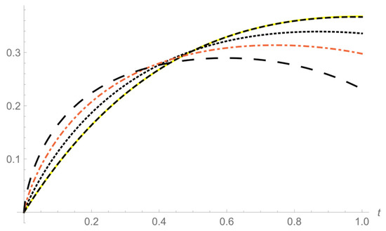
Figure 1.
The behavior of the sixth approximate solution of Equations (34) and (35) for different values of α. Solid line: exact solution at α = 1, dashed line: g6(t) at α = 1, dotted line: g6(t) at α = 0.9, dash. dotted line: g6(t) at α = 0.8, large dash. line: g6(t) at α = 0.7.
6. Conclusions
In the history of mathematics, there are several methods for solving differential equations, that have many applications in different fields of sciences and engineering. Recently, fractional differential equations have appeared, and many techniques have been developed to solve them. In this study, a combination of the ARA transform and the residual power series is implemented to solve fractional equations and other symmetric equations.
The efficiency of the method was shown by presenting two numerical examples and comparing the obtained results with other methods.
As a future work, we attend to extend the use of the ARA-RPSM to solve autonomous n-dimensional fractional nonlinear systems and to construct an equivalent method to solve partial fractional differential equations.
Author Contributions
Data curation, R.S., A.B. and A.Q.; Formal analysis, A.B., R.S. and A.Q.; Investigation, A.B., R.S. and A.Q.; Methodology, A.B., R.S. and A.Q.; Project administration, A.Q., R.S. and A.B.; Resources, A.B., R.S. and A.Q.; Writing—Original draft, A.Q., R.S. and A.B.; Writing—Review and editing, A.B., R.S. and A.Q. All authors have read and agreed to the published version of the manuscript.
Funding
This research is funded by the Deanship of Research at Zarqa University, Jordan.
Institutional Review Board Statement
Not applicable.
Informed Consent Statement
Not applicable.
Data Availability Statement
Not applicable.
Acknowledgments
The authors express their gratitude to the dear referees, who wish to remain anonymous, and the editor for their helpful suggestions, which improved the final version of this paper.
Conflicts of Interest
The authors declare no conflict of interest.
References
- Qazza, A.; Hatamleh, R.; Alodat, N. About the Solution Stability of Volterra Integral Equation with Random Kernel. Far East J. Math. Sci. 2016, 100, 671–680. [Google Scholar] [CrossRef]
- Pedrayes, J.F.; Melero, M.G.; Norniella, J.G.; Cabanas, M.F.; Orcajo, G.A.; González, A.S. Supercapacitors in Constant-Power Applications: Mathematical Analysis for the Calculation of Temperature. Appl. Sci. 2021, 11, 10153. [Google Scholar] [CrossRef]
- Qazza, A.; Hatamleh, R. The existence of a solution for semi-linear abstract differential equations with infinite B chains of the characteristic sheaf. Int. J. Appl. Math. 2018, 31, 611–620. [Google Scholar] [CrossRef]
- Arqub, O.A.; Al-Smadi, M.; Gdairi, R.A.; Alhodaly, M.; Hayat, T. Implementation of reproducing kernel Hilbert algorithm for pointwise numerical solvability of fractional Burgers’ model in time-dependent variable domain regarding constraint boundary condition of Robin. Results Phys. 2021, 24, 104210. [Google Scholar] [CrossRef]
- Ahmad, I.; Shah, K.; Rahman, G.U.; Baleanu, D. Stability analysis for a nonlinear coupled system of fractional hybrid delay differential equations. Math. Methods Appl. Sci. 2020, 43, 8669–8682. [Google Scholar] [CrossRef]
- Yang, X.; Qiu, Y.; Zhang, M.; Zhang, L.; Li, H. Facile Fabrication of Polyaniline/Graphene Composite Fibers as Electrodes for Fiber-Shaped Supercapacitors. Appl. Sci. 2021, 11, 8690. [Google Scholar] [CrossRef]
- Abu-Gdairi, R.; Hasan, S.; Al-Omari, S.; Al-Smadi, M.; Momani, S. Attractive Multistep Reproducing Kernel Approach for Solving Stiffness Differential Systems of Ordinary Differential Equations and Some Error Analysis. CMES 2021. in editing. [Google Scholar]
- Oldham, K.; Spanier, J. The Fractional Calculus: Theory and Applications of Differentiation and Integration to Arbitrary Order; Academic Press: New York, NY, USA, 1974. [Google Scholar]
- Podlubny, I. Fractional Differential Equations; Academic Press: San Diego, CA, USA, 1999. [Google Scholar]
- Mainardi, F. Fractional Calculus and Waves in Linear Viscoelasticity; Imperial College Press: London, UK, 2010. [Google Scholar]
- Almeida, R.; Tavares, D.; Torres, D. The Variable-Order Fractional Calculus of Variations; Springer: Cham, Switzerland, 2019. [Google Scholar]
- Miller, K.; Ross, B. An Introduction to the Fractional Calculus and Fractional Differential Equations; Wiley: New York, NY, USA, 1993. [Google Scholar]
- Adomian, G. Solving Frontier Problems of Physics: The Decomposition Method; Kluwer Academic Publisher: Boston, MA, USA, 1994. [Google Scholar]
- Jafari, H.; Daftardar–Gejji, V. Solving linear and nonlinear fractional diffusion and wave equations by Adomian decomposition. Appl. Math. Comput. 2006, 180, 488–497. [Google Scholar] [CrossRef]
- Saadeh, R. Numerical solutions of fractional convection-diffusion equation using finite-difference and finite-volume schemes. J. Math. Comput. Sci. 2021, 11, 7872–7891. [Google Scholar]
- He, J.H. Homotopy perturbation technique. Comput. Methods Appl. Mech. Eng. 1999, 178, 257–262. [Google Scholar] [CrossRef]
- Kashkari, B.S.; El–Tantawy, S.A.; Salas, A.H.; El-Sherif, L.S. Homotopy perturbation method for studying dissipative nonplanar solitons in an electronegative complex plasma. Chaos Solitons Fractals 2020, 130, 109457. [Google Scholar] [CrossRef]
- Saadeh, R. Numerical algorithm to solve a coupled system of fractional order using a novel reproducing kernel method. Alex. Eng. J. 2021, 60, 4583–4591. [Google Scholar] [CrossRef]
- Khandaqji, M.; Burqan, A. Results on sequential conformable fractional derivatives with applications. J. Comput. Anal. Appl. 2021, 29, 1115–1125. [Google Scholar]
- Abu-Gdairi, R.; Al-Smadi, M.; Gumah, G. An Expansion Iterative Technique for Handling Fractional Differential Equations Using Fractional Power Series Scheme. J. Math. Stat. 2015, 11, 29–38. [Google Scholar] [CrossRef]
- Khaminsou, B.; Sudsutad, W.; Thaiprayoon, C.; Alzabut, J.; Pleumpreedaporn, S. Analysis of Impulsive Boundary Value Pantograph Problems via Caputo Proportional Fractional Derivative under Mittag–Leffler Functions. Fractal Fract. 2021, 5, 251. [Google Scholar] [CrossRef]
- Burqan, A.; El-Ajou, A.; Saadeh, R.; Al-Smadi, M. A new efficient technique using Laplace transforms and smooth expansions to construct a series solutionsto the time-fractional Navier-Stokes equations. Alex. Eng. J. 2021, in press. [Google Scholar]
- Abbas, M.I.; Ragusa, M.A. On the Hybrid Fractional Differential Equations with Fractional Proportional Derivatives of a Function with Respect to a Certain Function. Symmetry 2021, 13, 264. [Google Scholar] [CrossRef]
- El-Ajou, A.; Oqielat, M.; Al-Zhour, Z.; Momani, S. A class of linear non-homogenous higher order matrix fractional differential equations: Analytical solutions and new technique. Fract. Calc. Appl. Anal. 2020, 23, 356–377. [Google Scholar] [CrossRef]
- Shqair, M.; El-Ajou, A.; Nairat, M. Analytical solution for multi-energy groups of neutron diffusion equations by a residual power series method. Mathematics 2019, 7, 633. [Google Scholar] [CrossRef]
- Ahmad, M.; Asjad, M.; Singh, J. Application of novel fractional derivative to heat and mass transfer analysis for the slippage flow of viscous fluid with single-wall carbon nanotube subject to Newtonian heating. Math. Meth. Appl Sci. 2021, 1–16. [Google Scholar] [CrossRef]
- Saadeh, R.; Qazza, A.; Burqan, A. A New Integral Transform: ARA Transform and Its Properties and Applications. Symmetry 2020, 12, 925. [Google Scholar] [CrossRef]
- Qazza, A.; Burqan, A.; Saadeh, R. A New Attractive Method in Solving Families of Fractional Differential Equations by a New Transform. Mathematics 2021, 9, 3039. [Google Scholar] [CrossRef]
- Mahmood, S.; Shah, R.; Khan, H.; Arif, M. Laplace Adomian decomposition method for multi-dimensional time fractional model of Navier-Stokes equation. Symmetry 2019, 11, 149. [Google Scholar] [CrossRef]
- Kumar, D.; Singh, J.; Kumar, S. A fractional model of Navier-Stokes equation arising in unsteady flow of a viscous fluid. J. Assoc. Arab Univ. Basic Appl. Sci. 2015, 17, 14–19. [Google Scholar] [CrossRef]
- Eriqat, T.; El-Ajou, A.; Moa’ath, N.O.; Al-Zhour, Z.; Momani, S. A new attractive analytic approach for solutions of linear and nonlinear neutral fractional pantograph equations. Chaos Solitons Fractals 2020, 138, 109957. [Google Scholar] [CrossRef]
- Magin, R.L. Fractional calculus models of complex dynamics in biological tissues. Comput. Math. Appl. 2010, 59, 1586–1593. [Google Scholar] [CrossRef]
- Sedaghat, S.; Ordokhani, Y.; Dehghan, M. Numerical solution of the delay differential equations of pantograph type via Chebyshev polynomials. Commun. Nonlinear Sci. Numer. Simul. 2012, 17, 4815–4830. [Google Scholar] [CrossRef]
- Balachandran, K.; Kiruthika, S. Existence of solutions of nonlinear fractional pantograph equations. Acta Math. Sci. 2013, 33, 712–720. [Google Scholar] [CrossRef]
- Bellen, A.; Zennaro, M. Numerical Methods for Delay Differential Equations. In Numerical Mathematics and Scientific Computation; The Clarendon Press: Oxford, UK; University Press: New York, NY, USA, 2003. [Google Scholar]
- Chen, X.; Wang, L. The variational iteration method for solving a neutral functional-differential equation with proportional delays. Comput. Math. Appl. 2010, 59, 2696–2702. [Google Scholar] [CrossRef]
- Rahimkhani, P.; Ordokhani, Y.; Babolian, E. Numerical solution of fractional pantograph differential equations by using generalized fractional-order Bernoulli wavelet. J. Comput. Appl. Math. 2017, 309, 493–510. [Google Scholar] [CrossRef]
- Hashemi, M.S.; Atangana, A.; Hajikhah, S. Solving fractional pantograph delay equations by an effective computational method. Math. Comput. Simul. 2020, 177, 295–305. [Google Scholar] [CrossRef]
- Ghasemi, M.; Fardi, M.; Ghaziani, R.K. Numerical solution of nonlinear delay differential equations of fractional order in reproducing kernel Hilbert space. Appl. Math. Comput. 2015, 268, 815–831. [Google Scholar] [CrossRef]
Publisher’s Note: MDPI stays neutral with regard to jurisdictional claims in published maps and institutional affiliations. |
© 2021 by the authors. Licensee MDPI, Basel, Switzerland. This article is an open access article distributed under the terms and conditions of the Creative Commons Attribution (CC BY) license (https://creativecommons.org/licenses/by/4.0/).