Worst-Case Higher Moment Coherent Risk Based on Optimal Transport with Application to Distributionally Robust Portfolio Optimization

Abstract

The tail risk management is of great significance in the investment process. As an extension of the asymmetric tail risk measure—Conditional Value at Risk (CVaR), higher moment coherent risk (HMCR) is compatible with the higher moment information (skewness and kurtosis) of probability distribution of the asset returns as well as capturing distributional asymmetry. In order to overcome the difficulties arising from the asymmetry and ambiguity of the underlying distribution, we propose the Wasserstein distributionally robust mean-HMCR portfolio optimization model based on the kernel smoothing method and optimal transport, where the ambiguity set is defined as a Wasserstein “ball” around the empirical distribution in the weighted kernel density estimation (KDE) distribution function family. Leveraging Fenchel’s duality theory, we obtain the computationally tractable DCP (difference-of-convex programming) reformulations and show that the ambiguity version preserves the asymmetry of the HMCR measure. Primary empirical test results for portfolio selection demonstrate the efficiency of the proposed model.

1. Introduction

Portfolio selection is a typical optimization problem under parameter uncertainty when facing uncertain asset returns. Unlike a deterministic optimization problem, the objective function in a decision model facing uncertainty is subjective and contingent on the preference of the investor. Indeed, investment preference concerning uncertainty can be associated with risk and ambiguity (see [1]). Following the seminal work by [2], the difference between the concepts of risk and ambiguity (Knightian uncertainty) in decision theory is that the former exposure to uncertain outcomes whose probability distribution is known, and the latter exposure to uncertainty about the probability distribution of the outcomes. Following the seminal work by [3], the portfolio selection is a bi-criteria optimization problem trading-off between returns and risk, that is, maximizing the expected portfolio return while, at the same time, minimizing some risk measure of portfolio loss. The assumption of distributional symmetry, however, is limiting in portfolio optimization, in which distributions are often known to be asymmetric. Thus, the downside risk measure that reflects asymmetric risk preferences is more suitable than variance that considers both upside and downside risk symmetrically in [3]. In this paper we focus on the following asymmetric tail risk measure—higher-moment coherent risk (HMCR) measures proposed by [4] (see [5] for more details of risk measure).

Definition 1

(HMCR). For any given confidence level $\gamma \in [0,1)$ and order $p\ge 1$, the HMCR measures of random loss X

$${\mathrm{HMCR}}_{\gamma }^p\left(X\right):=\underset{\alpha \in \mathbb{R}}{inf}\left\{\alpha +{(1-\gamma )}^{-1}{\parallel {[X-\alpha ]}_{+}\parallel }_p\right\},$$

(1)

where ${\left[x\right]}_{+}:=max\{x,0\}$ and ${\parallel X\parallel }_p:={\left(\mathbb{E}\left[{\left|X\right|}^p\right]\right)}^{1/p}$.

In particular, the popular Conditional Value-at-Risk (CVaR) corresponds to ${\mathrm{HMCR}}_{\gamma }^1$ (see [6]), and ${\mathrm{HMCR}}_{\gamma }^2$ is called the second-moment coherent risk (SMCR) measure. The following properties of the family of HMCR measures motivates us to choose it as the risk measure for portfolio selection: (i) In the sense of the coherent risk measure proposed by [7], HMCR measures are coherent and capture the distributional asymmetry. Furthermore, HMCR measures are compatible with second-order stochastic dominance (see [4]); (ii) As distinguished from the other known risk measures involving the information of the higher moments, for example, lower partial moment (see [8]) and the coherent measure of semi-${\mathcal{L}}_p$ type (see  [9]), the location of “tail cutoff” in the HMCR measures is determined by the optimal solution of the stochastic programming problem (1), meanwhile, is adjustable by the confidence level $\gamma$. (iii) The risk-aversion stochastic programming problem with HMCR measures can readily be handled by the well-developed methods of conic programming as the p-order cone within the positive orthant can be approximated by linear inequalities (see [4]).

Let the random asset returns $\mathit{\xi }\in {\mathbb{R}}^n$ be defined on a probability space ($\Omega ,\mathcal{F},\mathbb{P}$), where $\Omega$ is a compact sample space for $\mathit{\xi }$, $\mathcal{F}$ is a $\sigma$-algebra of $\Omega$, and $\mathbb{P}$ is a probability measure on $\mathcal{F}$. Let the portfolio decision be $\mathit{w}\in \mathcal{W}\subseteq {\mathbb{R}}^n$, where $\mathcal{W}$ represents a convex set of feasible decisions. For the given confidence level $\gamma \in [0,1)$ and the investor’s risk-aversion coefficient $\rho >0$, we consider the mean-HMCR portfolio optimization model of the following form:

$$\underset{\mathit{w}\in \mathcal{W},\alpha \in \mathbb{R}}{min}\left\{F(\mathit{w},\alpha ):=\rho \alpha +{\mathbb{E}}_P\left[-{\mathit{w}}^{\mathsf{T}}\mathit{\xi }\right]+\frac{\rho }{1-\gamma }{\left({\mathbb{E}}_P\left[{[-{\mathit{w}}^{\mathsf{T}}\mathit{\xi }-\alpha ]}_{+}^p\right]\right)}^{1/p}\right\},$$

(2)

where $\mathcal{W}=\{\mathit{w}:\mathit{w}\ge 0,{\mathbf{1}}^{\mathsf{T}}\mathit{w}=1\}$ and $\mathbf{1}$ denotes the vector of ones and P is the probability distribution of $\mathit{\xi }$. However, in real world the true probability distribution of $\mathit{\xi }$ is often unavailable, and is difficult to forecast precisely (see [10]), which results in poor out-of-sample performance when resorting to the sample average approximation (SAA) approach (see for example [11]). Thus, it makes sense to seek a robust portfolio immune to the uncertainty of distribution of the asset returns. Many powerful modeling paradigms have been proposed for optimization when facing uncertainty in the past decades (see for example [12,13,14]). The paradigm of distributionally robust optimization (DRO) considers an ambiguity set (a family of probability distributions with limited and known distributional information) and evaluates the performance of a decision-maker by its worst-case expected performance under any distribution residing in the ambiguity set, which may be traced to [15].

The key issue of DRO is how to construct an ambiguity set such that the bi-layer uncertain DRO model can be reformulated as a computationally tractable single-layer deterministic convex optimization problem. The popular methods of constructing an ambiguity set basically focus on the moment-based ambiguity set, which is constructed by certain moment information (see, for example, [16,17,18,19,20,21,22]), and the metric-based one, which is defined as a “ball” in the sense of a certain probability metric such as the Prohorov metric (see [23]), the goodness-of-fit (see [24]), likelihood function (see [25]), $\varphi$-divergence (see, for example,  [26,27,28,29,30]), Kullback–Leibler (KL) divergence (see, for example, [31,32]) and so forth. In particular, due to the outstanding properties of Wasserstein distance, defined as follows, Wasserstein distance is attracting a growing interest in DRO recently (see, for example, [33,34,35,36,37]).

Definition 2

(Wasserstein distance). For any $r\ge 1$, r-Wasserstein distance between two probability distributions Q and $Q^{\prime }$ on ${\mathbb{R}}^n$ is defined as:

$$W_r(Q,Q^{\prime })={\left(\underset{\pi \in \Pi (Q,Q^{\prime })}{inf}{\int }_{{\mathbb{R}}^n\times {\mathbb{R}}^n}{\parallel \mathit{\xi }-{\mathit{\xi }}^{\prime }\parallel }^r\pi (d\mathit{\xi },d{\mathit{\xi }}^{\prime })\right)}^{1/r},$$

(3)

where $\parallel ·\parallel$ is a norm on ${\mathbb{R}}^n$, while $\Pi (Q,Q^{\prime })$ denotes the set of all joint probability distributions of $\mathit{\xi }\in {\mathbb{R}}^n$ and ${\mathit{\xi }}^{\prime }\in {\mathbb{R}}^n$ with marginals Q and $Q^{\prime }$, respectively.

For example, ref. [33] study distributionally robust optimization problems with the Wasserstein ambiguity set centering at the empirical distribution and the objective of the inner maximization is an expectation of certain loss function, under certain mild assumptions, derive a finite convex programming problem. In this paper, we focus on the distributionally robust version of (2), that is, the following risk-aversion distributionally robust portfolio optimization model with the form:

$$\underset{\mathit{w}\in \mathcal{W},\alpha \in \mathbb{R}}{min}\underset{P\in \mathcal{P}}{max}\left\{F(\mathit{w},\alpha ;P):=\rho \alpha +{\mathbb{E}}_P\left[-{\mathit{w}}^{\mathsf{T}}\mathit{\xi }\right]+\frac{\rho }{1-\gamma }{\left({\mathbb{E}}_P\left[{[-{\mathit{w}}^{\mathsf{T}}\mathit{\xi }-\alpha ]}_{+}^p\right]\right)}^{1/p}\right\},$$

(4)

where the ambiguity set $\mathcal{P}$ is defined as a ball in the space of probability distribution by using Wasserstein distance, which is centered at the discrete empirical probability distribution. It is worth noting that, in contrast to the expected (risk-neutral) performance of certain loss function in the objective of the general DRO model (see, for example, [33,34,35,36,37]), the objective of (4) involve the risk-aversion performance—mean-HMCR, which is a nonlinear functional with respect to the probability distribution P. The nonliearity of the objective of the inner infinite-dimensional maximization optimization problem gives rise to a challenge, that is, it is difficult to solve the resulting semi-infinite optimization problem obtained by duality theory. Hence, to the best of our knowledge, it is difficult to derive the tractable reformulation of (4). From a statistical point of views, the mixture model in construction of ambiguity set can be treated as a parametric estimation model as the component distributions usually are predetermined (see [38,39]). However, in practice, the component distributions are unknown and can be obtained by historical simulation or expert predication, which motivates us to construct the Wasserstein ambiguity set by a nonparametric method in a data-driven setting in order to derive the computationally tractable reforumulation of (4).

The key contributions of our paper may be summarized as follows:

• To overcome the difficulties arise from the asymmetry and ambiguity of the underlying distribution, we propose a Wasserstein distributionally robust portfolio model based on kernel smoothing method and mean-HMCR, where the ambiguity set is a Wasserstein “ball” in the finite-dimensional probability distribution space spanned by the weighted KDE;
• Leveraging Optimal Transport theory, we define KDE–Wasserstein distance by incorporating KDE into Wasserstein distance and prove it enjoys a metric property;
• Leveraging Fenchel’s duality theory to obtain a finite-dimensional dual problem of the inner maximization problem, we overcome the difficulty arise from the nonliear functional with respect to probability distribution associated with HMCR, and derive the computationally tractability result of the Wasserstein distributionally robust portfolio model based on KDE and mean-HMCR.
• We extend $\varphi$-divergence ambiguity set in [40] to Wasserstein ambiguity set by integrating the weight KDE with Optimal Transport theory (see [41]), and we discover that the tractable reformulations of our model involve some difference-of-convex programming (DCP) constraints different from those of [40], which deeply reflects the insights arise from incorporating KDE into Wasserstein distance by optimal transport.

The remainder of this paper is organized as follows. Section 2 formally introduces the Wasserstein distributionally robust portfolio optimization based on KDE and mean-HMCR model, and obtains the computationally tractable reformulation of the corresponding DRO model by Fenchel’s duality theory. Section 3 presents numerical experiment of some empirical studies and sensitivity analysis on model parameters and Section 4 concludes.

2. Wasserstein Distributionally Robust Portfolio Optimization Based on KDE and Mean-HMCR

In this section, we propose a Wasserstein distributionally robust portfolio optimization model based on KDE and mean-HMCR, starting from giving an overview of traditional KDE and its variant—the weighted KDE, introducing the definition of KDE-Wasserstein distance by Optimal Transport theory (see [41]), and proposing new KDE-Wasserstein ambiguity set. Then the tractable reformulation of the corresponding DRO model is derived by Fenchel’s duality theory.

The kernel smoothing method has been a popular tool for the nonparametric estimation of the probability density function (PDF) $p(·)$ when the samples $X^1,\dots ,X^T$, which is typically assumed to be drawn independent and identically distributed (i.i.d.) from $p(·)$, are available. A kernel density estimator for a univariate PDF $p\left(x\right)$ is:

$$\widehat{p}\left(x\right):=\frac{1}{Th}\sum _{i=1}^{T}K\left(\frac{x-X^i}{h}\right)=\frac{1}{T}\sum _{i=1}^T{K}_h\left(x-X^i\right),$$

(5)

where the kernel function $K(·)$ plays the role of determining the shape of the “bumps” centred at each data point. The smoothing bandwidth $h>0$ controls the smoothness of the “bumps” and depends on the sample size T. Three popular assumptions on the kernel function $K(·)$ and the bandwidth $h=h\left(T\right)$ are listed as follows (see [42] for more details of KDE).

Assumption 1.

$K(·)\ge 0$ is bounded, $\int K\left(x\right)dx=1$.

Assumption 2.

$K(-x)=K\left(x\right)$ and $\int x^{p}K\left(x\right)dx<\infty ,p\ge 1$.

Assumption 3.

$h\left(T\right)\to 0$ and $Th\left(T\right)\to \infty$ as $T\to \infty$.

Although the Epanechnikov kernel is the optimal kernel function in the sense of the asymptotic mean integrated square error (MISE) with respect to $K(·)$, it has been known that MISE is quite insensitive to the shape of the kernel function (for example, Rectangular, Biweight, Triangular and Gaussian kernel functions). Thus, in practice, one generally chooses the Gaussian kernel for density estimation due to its smoothness. However, the selection of bandwidth h is of crucial importance for the high-performance density estimator. When the Gaussian kernel $K(·)$ is available and the estimated $p(·)$ is a Gaussian density with variance ${\sigma }^2$, then $h_{opt}=1.06\sigma T^{-1/5}$ would be the optimal bandwidth in MISE sense. See [42,43] for comprehensive reviews of the KDE.

Traditional KDE (5) is subject to bias that can mask structure by flattening peaks and filling in troughs in the density (see [44]), which contributes to the modifications to (5) that enjoy reduced bias while at the same time retaining the simple structure of (5). See, for example, the employment of high order kernels [45], variable bandwidth methodologies [46] and data sharpening [47]. An alternative reduced bias method can be obtained by replacing the local weights $T^{-1}$ in (5) with the global weights, $\mathit{\lambda }=({\lambda }_1,\dots ,{\lambda }_T)\in \Lambda$ and $\Lambda :=\{\mathit{\lambda }\in {\mathbb{R}}^T:{\mathbf{1}}^{\mathsf{T}}\mathit{\lambda }=1,\mathit{\lambda }\ge 0\}$, that is, the variant of KDE—the weighted KDE with the form:

$${\widehat{p}}_{\mathit{\lambda }}\left(x\right):=\sum _{i=1}^T{\lambda }_i{K}_h\left(x-X^i\right).$$

(6)

The rationality of the weighted KDE (6) is that the relative importance of different values of $X^i$ can be reflected by the “global” weights $\mathit{\lambda }$. Moreover, in some statistical applications, the weighted KDE (6) is readily integrated with additional information about $p(·)$ by the estimation equation (see [48,49,50] for more details of the weighted KDE). From a DRO point of view, it is important to incorporate the extra distributional information into the ambiguity set constructed by (6) such that the corresponding DRO model is less conservative. Hence the more flexible (6) motivates us to propose a new KDE-Wasserstein ambiguity set (9) by the Optimal Transport (see [41]). We define the following KDE-Wasserstein distance by integrating Wasserstein distance in (3) with the weighted KDE in (6).

Definition 3

(KDE-Wasserstein distance). For the given sample set $\{X^1,\dots ,X^T\}$, the KDE-Wasserstein distance between univariate distribution ${\widehat{p}}_{\mathit{\lambda }}$ and ${\widehat{p}}_{\mathit{\lambda }}$ in (6) is defined as follows.

$$d\left({\widehat{p}}_{\mathit{\lambda }},{\widehat{p}}_{\mathit{\lambda }}\right):=d_K\left(\mathit{\lambda },{\mathit{\lambda }}^{\prime }\right)={\left(\underset{\Pi \ge 0,}{min}\left\{\sum _{i=1}^T\sum _{j=1}^T{c}_{ij}^K{\pi }_{ij}|\sum _{j=1}^T{\pi }_{ij}={\lambda }_i,\forall i,\sum _{i=1}^T{\pi }_{ij}={\lambda }_j^{\prime },\forall j\right\}\right)}^{1/2},$$

(7)

where the transport cost $c_{ij}^K$ is taken to be the square of 2-Wasserstein distance in (3) between the i-th component $K^{\left(i\right)}(·)$ and the j-th component $K^{\left(j\right)}(·)$, that is, $c_{ij}^K:=W_2^2\left(K^{\left(i\right)}\left(x\right),K^{\left(j\right)}\left(x\right)\right)$ and $K^{\left(i\right)}\left(\mathit{x}\right):=K_h\left(x-X^i\right)$. In particular, for Gaussian kernel function $\varphi \left(x\right)=\left(1/\sqrt{2\pi }\right)e^{-x^2/2}$, the transport cost $c_{ij}^K$ in (7) admits a closed expression:

$$c_{ij}^{\varphi }={\left(X^i-X^j\right)}^2,i,j=1,\dots ,T.$$

(8)

Let $\mathcal{K}\left(\mathbb{R}\right)$ be the finite dimensional probability distribution function space spanned by (6).

Proposition 1.

Under Assumptions 1–3, $d\left(·,·\right)$ in (7) is a metric on $\mathcal{K}\left(\mathbb{R}\right)$.

Proof. 

It is easy to verify that $d\left({\widehat{p}}_{\mathit{\lambda }},{\widehat{p}}_{{\mathit{\lambda }}^{\prime }}\right)\ge 0$ for all ${\widehat{p}}_{\mathit{\lambda }},{\widehat{p}}_{{\mathit{\lambda }}^{\prime }}\in \mathcal{K}\left(\mathbb{R}\right)$ and $d\left({\widehat{p}}_{\mathit{\lambda }},{\widehat{p}}_{{\mathit{\lambda }}^{\prime }}\right)=0$ if and only if ${\widehat{p}}_{\mathit{\lambda }}={\widehat{p}}_{\mathit{\mu }}$. We prove the triangular inequality $d\left({\widehat{p}}_{\mathit{\lambda }},{\widehat{p}}_{{\mathit{\lambda }}^{\prime }}\right)\le d\left({\widehat{p}}_{\mathit{\lambda }},{\widehat{p}}_{\mathit{\mu }}\right)+d\left({\widehat{p}}_{\mathit{\mu }},{\widehat{p}}_{{\mathit{\lambda }}^{\prime }}\right)$ for all ${\widehat{p}}_{\mathit{\lambda }},{\widehat{p}}_{\mathit{\mu }},{\widehat{p}}_{{\mathit{\lambda }}^{\prime }}\in \mathcal{K}\left(\mathbb{R}\right)$. Let ${\Pi }^{\mathit{\lambda }\mathit{\mu }}$ (${\Pi }^{\mathit{\mu }{\mathit{\lambda }}^{\prime }}$) be the solution of problem (7) with marginals ${\widehat{p}}_{\mathit{\lambda }},{\widehat{p}}_{\mathit{\mu }}$ (${\widehat{p}}_{\mathit{\mu }},{\widehat{p}}_{{\mathit{\lambda }}^{\prime }}$) and define ${\Pi }^{\mathit{\lambda }{\mathit{\lambda }}^{\prime }}$ by ${\pi }_{i,k}^{\mathit{\lambda }{\mathit{\lambda }}^{\prime }}:={\sum }_{j=1}^T\frac{{\pi }_{ij}^{\mathit{\lambda }\mathit{\mu }}{\pi }_{jk}^{\mathit{\mu }{\mathit{\lambda }}^{\prime }}}{{\mu }_j}.$ For given $i=1,\dots ,T$, we have

$$\sum _{k=1}^T{\pi }_{i,k}^{\mathit{\lambda }{\mathit{\lambda }}^{\prime }}=\sum _{k=1}^T\left(\sum _{j=1}^T\frac{{\pi }_{ij}^{\mathit{\lambda }\mathit{\mu }}{\pi }_{jk}^{\mathit{\mu }{\mathit{\lambda }}^{\prime }}}{{\mu }_j}\right)=\sum _{j=1}^T\frac{{\pi }_{ij}^{\mathit{\lambda }\mathit{\mu }}\left({\sum }_{k=1}^T{\pi }_{jk}^{\mathit{\mu }{\mathit{\lambda }}^{\prime }}\right)}{{\mu }_j}=\sum _{j=1}^T{\pi }_{i,j}^{\mathit{\lambda }{\mathit{\lambda }}^{\prime }}={\lambda }_i.$$

Similarly, for given $k=1,\dots ,T$, we have ${\sum }_{i=1}^T{\pi }_{i,k}^{\mathit{\lambda }{\mathit{\lambda }}^{\prime }}={\mathit{\lambda }}_k^{\prime }.$ Thus, ${\Pi }^{\mathit{\lambda }{\mathit{\lambda }}^{\prime }}$ is a joint probability distribution between $\mathit{\lambda }$ and ${\mathit{\lambda }}^{\prime }$. Therefore,

$$\begin{array}{cc}\hfill d\left({\widehat{p}}_{\mathit{\lambda }},{\widehat{p}}_{{\mathit{\lambda }}^{\prime }}\right)& \le {\left(\sum _{i,k}{\pi }_{ik}^{\mathit{\lambda }{\mathit{\lambda }}^{\prime }}{\left(W_2\left(K^{\left(i\right)},K^{\left(k\right)}\right)\right)}^2\right)}^{1/2}\hfill \\ & ={\left(\sum _{i,j,k}\frac{{\pi }_{ij}^{\mathit{\lambda }\mathit{\mu }}{\pi }_{jk}^{\mathit{\mu }{\mathit{\lambda }}^{\prime }}}{{\mu }_j}{\left(W_2\left(K^{\left(i\right)},K^{\left(k\right)}\right)\right)}^2\right)}^{1/2}\hfill \\ & \le {\left(\sum _{i,j,k}\frac{{\pi }_{ij}^{\mathit{\lambda }\mathit{\mu }}{\pi }_{jk}^{\mathit{\mu }{\mathit{\lambda }}^{\prime }}}{{\mu }_j}{\left(W_2\left(K^{\left(i\right)},K^{\left(j\right)}\right)+W_2\left(K^{\left(j\right)},K^{\left(k\right)}\right)\right)}^2\right)}^{1/2}\hfill \\ & \le {\left(\sum _{i,j,k}\frac{{\pi }_{ij}^{\mathit{\lambda }\mathit{\mu }}{\pi }_{jk}^{\mathit{\mu }{\mathit{\lambda }}^{\prime }}}{{\mu }_j}{\left(W_2\left(K^{\left(i\right)},K^{\left(j\right)}\right)\right)}^2\right)}^{1/2}+{\left(\sum _{i,j,k}\frac{{\pi }_{ij}^{\mathit{\lambda }\mathit{\mu }}{\pi }_{jk}^{\mathit{\mu }{\mathit{\lambda }}^{\prime }}}{{\mu }_j}{\left(W_2\left(K^{\left(j\right)},K^{\left(k\right)}\right)\right)}^2\right)}^{1/2}\hfill \\ & ={\left(\sum _{i,j}{\pi }_{ij}^{\mathit{\lambda }\mathit{\mu }}{\left(W_2\left(K^{\left(i\right)},K^{\left(j\right)}\right)\right)}^2\right)}^{1/2}+{\left(\sum _{j,k}{\pi }_{jk}^{\mathit{\mu }{\mathit{\lambda }}^{\prime }}{\left(W_2\left(K^{\left(j\right)},K^{\left(k\right)}\right)\right)}^2\right)}^{1/2}\hfill \\ & =d\left({\widehat{p}}_{\mathit{\lambda }},{\widehat{p}}_{\mathit{\mu }}\right)+d\left({\widehat{p}}_{\mathit{\mu }},{\widehat{p}}_{{\mathit{\lambda }}^{\prime }}\right),\hfill \end{array}$$

where the second inequality holds due to the fact $W_2(·,·)$ is a metric, and the third inequality holds from the Minkowski inequality. □

By KDE–Wasserstein distance (7), the KDE-Wasserstein ambiguity set of the univariate random variable X associated with the samples $X^1,\dots ,X^T$ is obtained.

Definition 4

(KDE-Wasserstein ambiguity set). For the given sample set $\{X^1,\dots ,X^T\}$, the KDE-Wasserstein ambiguity set of X is defined as follows.

$${\mathcal{P}}_{d_K}^{\tau }:=\left\{{\widehat{p}}_{\mathit{\lambda }}=\sum _{i=1}^T{\lambda }_i{K}_h\left(x-X^i\right)|\mathit{\lambda }\in {\Lambda }_{d_K}^{\tau }\right\},$$

(9)

where ${\Lambda }_{d_K}^{\tau }:=\left\{\mathit{\lambda }\right|\mathit{\lambda }\in \Lambda ,d_K(\mathit{\lambda },{\mathit{\lambda }}^0)\le \tau \}$ and ${\mathit{\lambda }}^0:=(1/T)\mathbf{1}$. The radius of the ambiguity set $\tau \ge 0$ controls the degree of the distributional uncertainty.

Due to the two facts: (i) from a statistical point of view, the multivariate KDE for the continuous PDF of the asset returns gives rise to “curse of dimensionality” (see, for example, [42]); (ii) from an optimization point of view, the closed formulation associated with HMCR measure in the objective function of problem (2) can not be obtained by using the multivariate weighted KDE since the multiple integration of positive function with respect to the multivariate weighted KDE is hard to be calculated, we estimate the univariate PDF of the random portfolio loss by using the univariate weighted KDE (6) rather than estimating multivariate PDF of the random asset returns by using the multivariate weighted KDE. For the given sample set $\{{\mathit{\xi }}^1,\dots ,{\mathit{\xi }}^T\}$ of random asset returns $\mathit{\xi }\in \Omega$, which is typically assumed to be drawn i.i.d. from the probability function P of $\mathit{\xi }$, the corresponding sample set of the portfolio loss $\{-{\mathit{w}}^{\mathsf{T}}{\mathit{\xi }}^1,\dots ,-{\mathit{w}}^{\mathsf{T}}{\mathit{\xi }}^T\}$ is obtained. For any fixed portfolio decision $\mathit{w}\in \mathcal{W}$, the KDE-Wasserstein ambiguity set of the portfolio loss $-{\mathit{w}}^{\mathsf{T}}\mathit{\xi }$ can be derived

$${\mathcal{P}}_{d_K}^{\tau }=\left\{{\widehat{p}}_{\mathit{\lambda }}=\sum _{i=1}^T{\lambda }_i{K}_h\left(x+{\mathit{w}}^{\mathsf{T}}{\mathit{\xi }}^i\right)|\mathit{\lambda }\in {\Lambda }_{d_K}^{\tau }\right\},$$

(10)

where ${\Lambda }_{d_K}^{\tau }=\left\{\mathit{\lambda }\right|\mathit{\lambda }\in \Lambda ,d_K(\mathit{\lambda },{\mathit{\lambda }}^0)\le \tau \}$ and ${\mathit{\lambda }}^0=(1/T){\mathbf{1}}^{\mathsf{T}}$. When Gaussian kernel function $\varphi \left(x\right)=\left(1/\sqrt{2\pi }\right)e^{-x^2/2}$ is available, the transport cost $c_{ij}^K$ in (10) admits a closed expression by (8):

$$c_{ij}^{\varphi }=c_{ij}^{\varphi }\left(\mathit{w}\right)={\left({\mathit{w}}^{\mathsf{T}}{\mathit{\xi }}^i-{\mathit{w}}^{\mathsf{T}}{\mathit{\xi }}^j\right)}^2,i,j=1,\dots ,T.$$

(11)

By replacing the Wasserstein ambiguity set $\mathcal{P}$ in (4) with the KDE-Wasserstein ambiguity set ${\mathcal{P}}_{d_K}^{\tau }$ in (10), we propose the Wasserstein distributionally robust portfolio optimization model based on KDE and mean-HMCR.

$$\underset{\mathit{w}\in \mathcal{W},\alpha \in \mathbb{R}}{min}\underset{P\in {\mathcal{P}}_{d_K}^{\tau }}{max}\left\{F(\mathit{w},\alpha ;P)=\rho \alpha +{\mathbb{E}}_P\left[-{\mathit{w}}^{\mathsf{T}}\mathit{\xi }\right]+\frac{\rho }{1-\gamma }{\left({\mathbb{E}}_P\left[{[-{\mathit{w}}^{\mathsf{T}}\mathit{\xi }-\alpha ]}_{+}^p\right]\right)}^{1/p},\right\},$$

(12)

where the confidence level $\gamma \in [0,1)$, risk coefficient $\rho >0$, kernel function $K(·)$, bandwidth $h>0$, the weights $\mathit{\lambda }\in \Lambda$ and $p\ge 1$ are given. It follows from (10) that the objective function of (12) admits a closed expression. Hence problem (12) is equivalent to:

$$\underset{\mathit{w}\in \mathcal{W},\alpha \in \mathbb{R}}{min}\underset{\mathit{\lambda }\in {\Lambda }_{d_K}^{\tau }}{max}\left\{{\widehat{F}}_K(\mathit{w},\alpha ;\mathit{\lambda })=\rho \alpha -\sum _{i=1}^T{\lambda }_i{\mathit{w}}^{\mathsf{T}}{\mathit{\xi }}^i+\frac{\rho }{1-\gamma }{\left(\sum _{i=1}^T{\lambda }_i{\Phi }_p^p(-{\mathit{w}}^{\mathsf{T}}{\mathit{\xi }}^i-\alpha ,h)\right)}^{1/p}\right\},$$

(13)

where ${\Phi }_p(x,h)=\left({\phi }_{p}h\right)\left(x\right):=h{\phi }_p\left(h^{-1}x\right)$, ${\phi }_p\left(x\right)={\left(G_p\left(x\right)\right)}^{1/p}$, $G_p\left(x\right)={\int }_{-\infty }^x{(x-t)}^{p}K\left(t\right)dt$ for $p\ge 1$, $\left({\phi }_{p}h\right)\left(x\right)$ is called a perspective function or an operation of right multiplication (see [51] (pp. 34–35)). ${\Phi }_p(x,h)$ is jointly convex satisfying $\nabla {\Phi }_p(x,h)\ge 0$, and ${\left[x\right]}_{+}$ is the recession function $\left({\phi }_p{0}_{+}\right)\left(x\right)$ of ${\phi }_p\left(x\right)$ (see [51] (pp. 66–67)), ${\Phi }_p(x,h)={\left[x\right]}_{+}+o\left(h\right)$ for $x\ne 0$ and ${\Phi }_p(0,h)=O\left(h\right)$ (see [40]).

We prove the tractability result of the Wasserstein distributionally robust portfolio optimization based on the KDE and mean-${\mathrm{HMCR}}_{\gamma }^p$ model (12), starting from giving the following Lemma 1 in [30]. The relative interior of a set $\mathcal{U}$ and $\{\mathit{x}\in {\mathbb{R}}^N,\mathit{x}>0\}$ are denoted by $\mathrm{ri}\left(\mathcal{U}\right)$ and ${\mathbb{R}}_{++}^N$, respectively.

Lemma 1.

([30] (Theorem 1)) Let $f:{\mathbb{R}}^M\times {\mathbb{R}}_{+}^N\mapsto \mathbb{R}$ be a function such that $f(\mathit{w},·)$ is closed and concave for each $\mathit{w}\in {\mathbb{R}}^M$. Consider a constraint of the form:

$$f(\mathit{w},\mathit{p})\le \beta ,\forall \mathit{p}\in \mathcal{U},$$

(14)

where $\mathcal{U}$ is such that:

$$\mathrm{ri}\left(\mathcal{U}\right)\cap {\mathbb{R}}_{++}^N\ne ⌀,$$

Constraint (14) holds for any given $\mathit{w}$ if and only if:

$$\exists \mathit{v}\in {\mathbb{R}}^N:{\delta }^{\ast }\left(\mathit{v}\right|\mathcal{U})-f_{\ast }(\mathit{w},\mathit{v})\le \beta ,$$

where ${\delta }^{\ast }\left(\mathit{v}\right|\mathcal{U}):=\underset{\mathit{p}\in \mathcal{U}}{sup}{\mathit{v}}^{\mathsf{T}}\mathit{p}$, which is the support function of $\mathcal{U}$, and $f_{\ast }(\mathit{w},\mathit{v}):=$$\underset{\mathit{p}\ge 0}{inf}\left\{{\mathit{v}}^{\mathsf{T}}\mathit{p}-f(\mathit{w},\mathit{p})\right\}$, which is the concave conjugate function of $f(\mathit{w},\mathit{p})$ with respect to its second argument.

We then prove the tractable reformulation of the Wasserstein distributionally robust portfolio optimization based on KDE and mean-${\mathrm{HMCR}}_{\gamma }^p$ model (12) with given ${\mathit{\xi }}^i,i=1,\dots ,T$, $\gamma \in [0,1)$, $\rho >0$, $h>0$, $p>1$ and $\tau >0$.

Theorem 1.

Problem (12) is equivalent to the following optimization problem:

$$\begin{array}{cc}min& {\tau }^2\zeta +\eta +{\mathit{\beta }}^{\mathsf{T}}{\mathit{\lambda }}^0+\rho \alpha -{\left(\frac{\rho }{p(1-\gamma )}\right)}^{\frac{p}{p-1}}(1-p)y\hfill \\ \mathrm{s}.\mathrm{t}.& \frac{{\left({\Phi }_p(-{\mathit{w}}^{\mathsf{T}}{\mathit{\xi }}^i-\alpha ,h)\right)}^p}{y^{p-1}}-{\mathit{w}}^{\mathsf{T}}{\mathit{\xi }}^i-c_{ij}^K\left(\mathit{w}\right)\zeta \le \eta +{\beta }_j,i,j=1,\dots ,T,\hfill \\ & \mathit{w}\in \mathcal{W},\alpha \in \mathbb{R},\eta \in \mathbb{R},\zeta \in {\mathbb{R}}_{+},y\in {\mathbb{R}}_{+},\mathit{\beta }\in {\mathbb{R}}^T.\hfill \end{array}$$

(15)

Furthermore, (15) is formulated as:

$$\underset{\mathit{w}\in \mathcal{W},\alpha \in \mathbb{R},\zeta \in {\mathbb{R}}_{+},y\in {\mathbb{R}}_{+}}{min}\left\{{\tau }^2\zeta +\frac{1}{T}\sum _{j=1}^T{f}_j^K(\mathit{w},\alpha ,\zeta ,y)+\rho \alpha -{\left(\frac{\rho }{p(1-\gamma )}\right)}^{\frac{p}{p-1}}(1-p)y\right\},$$

(16)

where $f_j^K(\mathit{w},\alpha ,\zeta ,y)=\underset{i=1,\dots ,T}{max}\left\{\frac{{\left({\Phi }_p(-{\mathit{w}}^{\mathsf{T}}{\mathit{\xi }}^i-\alpha ,h)\right)}^p}{y^{p-1}}-{\mathit{w}}^{\mathsf{T}}{\mathit{\xi }}^i-c_{ij}^K\left(\mathit{w}\right)\zeta \right\}$.

In particular, when Gaussian kernel function $\varphi \left(x\right)=(1/\sqrt{2\pi })e^{-x^2/2}$ is available, problem (16) is equivalent to the following DCP problem:

$$\underset{\mathit{w}\in \mathcal{W},\alpha \in \mathbb{R},\zeta \in {\mathbb{R}}_{+},y\in {\mathbb{R}}_{+}}{min}\left\{\frac{{\tau }^2}{\zeta }+\frac{1}{T}\sum _{j=1}^T{f}_j^{\varphi }(\mathit{w},\alpha ,\zeta ,y)+\rho \alpha -{\left(\frac{\rho }{p(1-\gamma )}\right)}^{\frac{p}{p-1}}(1-p)y\right\},$$

(17)

where $f_j^{\varphi }(\mathit{w},\alpha ,\zeta ,y)=\underset{i=1,\dots ,T}{max}\left\{\frac{{\left({\Phi }_p(-{\mathit{w}}^{\mathsf{T}}{\mathit{\xi }}^i-\alpha ,h)\right)}^p}{y^{p-1}}-{\mathit{w}}^{\mathsf{T}}{\mathit{\xi }}^i-\frac{c_{ij}^{\varphi }\left(\mathit{w}\right)}{\zeta }\right\}$ and $c_{ij}^{\varphi }\left(\mathit{w}\right)={({\mathit{w}}^{\mathsf{T}}{\mathit{\xi }}^i-{\mathit{w}}^{\mathsf{T}}{\mathit{\xi }}^j)}^2$.

Proof. 

By (13) and introducing the epigraph variable $\nu \in \mathbb{R}$, we have that problem (12) is equivalent to:

$$\begin{array}{ccc}\underset{\mathit{w}\in \mathcal{W},\alpha \in \mathbb{R},\nu \in \mathbb{R}}{min}& \nu ,\hfill & \\ \mathrm{s}.\mathrm{t}.& {\widehat{F}}_K(\mathit{w},\alpha ;\mathit{\lambda })\le \nu ,\hfill & \hfill \forall \mathit{\lambda }\in {\Lambda }_{d_K}^{\tau }.\end{array}$$

(18)

According to Lemma 1, for any given $\mathit{w}$, $\alpha$ and $\nu$, the constraint in (18) holds if and only if:

$$\exists \mathit{v}\in {\mathbb{R}}^T:{\delta }^{\ast }\left(\mathit{v}\right|{\Lambda }_{\varphi }^{\tau })-{\left({\widehat{F}}_K\right)}_{\ast }(\mathit{w},\alpha ;\mathit{v})\le \nu .$$

(19)

In order to obtain the computationally tractable reformulation of problem (12), we need to derive the closed expressions of the support function of the uncertainty set ${\Lambda }_{d_K}^{\tau }$ in (9) and the concave conjugate function of ${\widehat{F}}_K(\mathit{w},\alpha ;·)$ in (19).

On the one hand, let ${\tilde{\Lambda }}_{d_K}^{\tau }$ be the extended version of ${\Lambda }_{d_K}^{\tau }$,

$${\tilde{\Lambda }}_{d_K}^{\tau }:=\{\tilde{\mathit{\lambda }}|\tilde{\mathit{\lambda }}\ge 0,{\mathbf{1}}^{\mathsf{T}}\mathit{\lambda }=1,\sum _{i,j}{c}_{ij}^K\left(\mathit{w}\right){\pi }_{ij}\le {\tau }^2,\sum _j{\pi }_{ij}-{\lambda }_i=0,i=1,\dots ,T,\sum _i{\pi }_{ij}={\lambda }_j^0,j=1,\dots ,T\},$$

where $\tilde{\mathit{\lambda }}:={\left({\mathit{\lambda }}^{\mathsf{T}},{\pi }_{11},{\pi }_{12},\dots ,{\pi }_{1T},\cdots ,{\pi }_{T1},{\pi }_{T2},\dots ,{\pi }_{TT}\right)}^{\mathsf{T}}\in {\mathbb{R}}^{T(1+T)}$. From the duality theorem of linear programming problem, we have:

$$\begin{array}{cc}\hfill {\delta }^{\ast }\left(\mathit{v}|{\tilde{\Lambda }}_{d_K}^{\tau }\right)& =\left\{\underset{\mathit{\lambda }\ge 0,\Pi \ge 0}{max}{\mathit{v}}^{\mathsf{T}}\mathit{\lambda }\left|\begin{array}{cc}\hfill & {\mathbf{1}}^{\mathsf{T}}\mathit{\lambda }=1,\hfill \\ \hfill & \sum _{i=1}^T\sum _{j=1}^T{c}_{ij}^K\left(\mathit{w}\right){\pi }_{ij}\le {\tau }^2,\hfill \\ \hfill & \sum _{j=1}^T{\pi }_{ij}-{\lambda }_i=0,i=1,\dots ,T,\hfill \\ \hfill & \sum _{i=1}^T{\pi }_{ij}={\lambda }_j^0,j=1,\dots ,T,\hfill \end{array}\right.\right\}\hfill \\ \hfill & =\left\{min\eta +{\tau }^2\zeta +{\mathit{\beta }}^{\mathsf{T}}{\mathit{\lambda }}^0\left|\begin{array}{cc}\hfill & \eta -{\theta }_i\ge v_i,i=1,\dots ,T,\hfill \\ \hfill & c_{ij}^K\left(\mathit{w}\right)\zeta +{\theta }_i+{\beta }_j\ge 0,i,j=1,\dots ,T,\hfill \\ \hfill & \eta \in \mathbb{R},\zeta \ge 0,\mathit{\theta }\in {\mathbb{R}}^T,\mathit{\beta }\in {\mathbb{R}}^T.\hfill \end{array}\right.\right\}\hfill \end{array}$$

(20)

On the other hand, it is obvious to derive that the concave conjugate function of $f\left(x\right)=\frac{x^p}{p},x\ge 0,0<p<1$, has closed formulation $f_{\ast }\left(y\right)=\frac{y^q}{q},y\ge 0$, where $1/p+1/q=1$ (see [52]). From [51] (Theorem 16.3) we have the concave conjugate function of ${\widehat{F}}_K(\mathit{w},\alpha ;·)$ in (19):

$$\begin{array}{cc}\hfill {\left({\widehat{F}}_K\right)}_{\ast }(\mathit{w},\alpha ;\mathit{v})=& \underset{z\ge 0}{sup}\left\{-\rho \alpha +{\left(\frac{\rho }{p(1-\gamma )}\right)}^{\frac{p}{p-1}}(1-p)z^{\frac{1}{1-p}}:\right.\hfill \\ \hfill & \left.z\left(\begin{array}{c}{\left({\Phi }_p\left(-{\mathit{w}}^{\mathsf{T}}{\mathit{\xi }}^1-\alpha ,h\right)\right)}^p\\ ⋮\\ {\left({\Phi }_p\left(-{\mathit{w}}^{\mathsf{T}}{\mathit{\xi }}^T-\alpha ,h\right)\right)}^p\end{array}\right)=\left(\begin{array}{c}{v}_1+{\mathit{w}}^{\mathsf{T}}{\mathit{\xi }}^1\\ ⋮\\ v_T+{\mathit{w}}^{\mathsf{T}}{\mathit{\xi }}^T\end{array}\right).\right\}\hfill \end{array}$$

(21)

Replacing $1/z$ in (21) with analysis variable s gives rise to:

$$\begin{array}{cc}\hfill {\left({\widehat{F}}_K\right)}_{\ast }(\mathit{w},\alpha ;\mathit{v})=& \underset{s\ge 0}{sup}\left\{-\rho \alpha +{\left(\frac{\rho }{p(1-\gamma )}\right)}^{\frac{p}{p-1}}(1-p)s^{\frac{1}{p-1}}:\right.\hfill \\ \hfill & \left.s^{-1}{\left({\Phi }_p\left(-{\mathit{w}}^{\mathsf{T}}{\mathit{\xi }}^i-\alpha ,h\right)\right)}^p=v_i+{\mathit{w}}^{\mathsf{T}}{\mathit{\xi }}^i,i=1,\dots ,T.\right\}\hfill \end{array}$$

Furthermore, we have

$$\begin{array}{cc}\hfill {\left({\widehat{F}}_K\right)}_{\ast }(\mathit{w},\alpha ;\mathit{v})=& \underset{s\ge 0}{sup}\left\{-\rho \alpha +{\left(\frac{\rho }{p(1-\gamma )}\right)}^{\frac{p}{p-1}}(1-p)s^{\frac{1}{p-1}}:\right.\hfill \\ \hfill & \left.s^{-1}{\left({\Phi }_p\left(-{\mathit{w}}^{\mathsf{T}}{\mathit{\xi }}^i-\alpha ,h\right)\right)}^p\le v_i+{\mathit{w}}^{\mathsf{T}}{\mathit{\xi }}^i,i=1,\dots ,T.\right\}\hfill \\ \hfill =& \underset{y\ge 0}{sup}\left\{-\rho \alpha +{\left(\frac{\rho }{p(1-\gamma )}\right)}^{\frac{p}{p-1}}(1-p)y:\right.\hfill \\ \hfill & \left.\frac{{\left({\Phi }_p\left(-{\mathit{w}}^{\mathsf{T}}{\mathit{\xi }}^i-\alpha ,h\right)\right)}^p}{y^{p-1}}\le v_i+{\mathit{w}}^{\mathsf{T}}{\mathit{\xi }}^i,i=1,\dots ,T,\right\}\hfill \end{array}$$

where the first equality holds due to the fact that the functions of s in the objective and the left-hand side of the constraints are all decreasing with respect to s, and the second equality holds by replacing $s^{\frac{1}{p-1}}$ with y. Combining (20) with (18), it follows from Lemma 1 that:

$$\left\{\begin{array}{c}\eta +{\tau }^2\zeta +{\mathit{\beta }}^{\mathsf{T}}{\mathit{\lambda }}^0+\rho \alpha -{\left(\frac{\rho }{p(1-\gamma )}\right)}^{\frac{p}{p-1}}(1-p)y\le \nu ,\hfill \\ \frac{{\left({\Phi }_p(-{\mathit{w}}^{\mathsf{T}}{\mathit{\xi }}^i-\alpha ,h)\right)}^p}{y^{p-1}}-{\mathit{w}}^{\mathsf{T}}{\mathit{\xi }}^i\le v_i,i=1,\dots ,T,\hfill \\ \eta -{\theta }_i\ge v_i,i=1,\dots ,T,\hfill \\ c_{ij}^K\left(\mathit{w}\right)\zeta +{\theta }_i+{\beta }_j\ge 0,i,j=1,\dots ,T,\hfill \\ \mathit{w}\in \mathcal{W},\alpha \in \mathbb{R},\nu \in \mathbb{R},\eta \in \mathbb{R},\zeta \in {\mathbb{R}}_{+},y\in {\mathbb{R}}_{+},\mathit{\theta }\in {\mathbb{R}}^T,\mathit{\beta }\in {\mathbb{R}}^T,\mathit{v}\in {\mathbb{R}}^T.\hfill \end{array}\right.$$

(22)

It is easy to verify that the second group of constraints in (22) are jointly convex on $\mathit{w},\alpha ,y,v_i,i=1,\dots ,T$, which can be solved by geometric programming (see [53]). Eliminating $\mathit{v}$ from (22) , we get:

$$\left\{\begin{array}{c}\eta +{\tau }^2\zeta +{\mathit{\beta }}^{\mathsf{T}}{\mathit{\lambda }}^0+\rho \alpha -{\left(\frac{\rho }{p(1-\gamma )}\right)}^{\frac{p}{p-1}}(1-p)y\le \nu ,\hfill \\ \frac{{\left({\Phi }_p(-{\mathit{w}}^{\mathsf{T}}{\mathit{\xi }}^i-\alpha ,h)\right)}^p}{y^{p-1}}-{\mathit{w}}^{\mathsf{T}}{\mathit{\xi }}^i\le \eta -{\theta }_i,i=1,\dots ,T,\hfill \\ c_{ij}^K\left(\mathit{w}\right)\zeta +{\beta }_j\ge -{\theta }_i,i,j=1,\dots ,T,\hfill \\ \mathit{w}\in \mathcal{W},\alpha \in \mathbb{R},\eta \in \mathbb{R},\zeta \in {\mathbb{R}}_{+},y\in {\mathbb{R}}_{+},\mathit{\theta }\in {\mathbb{R}}^T,\mathit{\beta }\in {\mathbb{R}}^T,\mathit{v}\in {\mathbb{R}}^T.\hfill \end{array}\right.$$

(23)

Furthermore, eliminating $\mathit{\theta }$ from (23), we get:

$$\left\{\begin{array}{c}\eta +{\tau }^2\zeta +{\mathit{\beta }}^{\mathsf{T}}{\mathit{\lambda }}^0+\rho \alpha -{\left(\frac{\rho }{p(1-\gamma )}\right)}^{\frac{p}{p-1}}(1-p)y\le \nu ,\hfill \\ \frac{{\left({\Phi }_p(-{\mathit{w}}^{\mathsf{T}}{\mathit{\xi }}^i-\alpha ,h)\right)}^p}{y^{p-1}}-{\mathit{w}}^{\mathsf{T}}{\mathit{\xi }}^i-c_{ij}^K\left(\mathit{w}\right)\zeta \le \eta +{\beta }_j,i,j=1,\dots ,T,\hfill \\ \mathit{w}\in \mathcal{W},\alpha \in \mathbb{R},\nu \in \mathbb{R},\eta \in \mathbb{R},\zeta \in {\mathbb{R}}_{+},y\in {\mathbb{R}}_{+},\mathit{\theta }\in {\mathbb{R}}^T,\mathit{\beta }\in {\mathbb{R}}^T,\mathit{v}\in {\mathbb{R}}^T,\hfill \end{array}\right.$$

(24)

which leads to the tractable reformulation (15) of problem (12).

Denote $\underset{i=1,\dots ,T}{max}\left\{\frac{{\left({\Phi }_p(-{\mathit{w}}^{\mathsf{T}}{\mathit{\xi }}^i-\alpha ,h)\right)}^p}{y^{p-1}}-{\mathit{w}}^{\mathsf{T}}{\mathit{\xi }}^i-c_{ij}^K\left(\mathit{w}\right)\zeta \right\}$ by $f_j^K(\mathit{w},\alpha ,\zeta ,y),j=1,\dots ,T$, and eliminating $\eta ,\mathit{\beta }$ from (24), we have:

$$\left\{\begin{array}{c}{\tau }^2\zeta +\frac{1}{T}\sum _{j=1}^T{f}_j^K(\mathit{w},\alpha ,\zeta ,y)+\rho \alpha -{\left(\frac{\rho }{p(1-\gamma )}\right)}^{\frac{p}{p-1}}(1-p)y\le \nu ,\hfill \\ \mathit{w}\in \mathcal{W},\alpha \in \mathbb{R},\nu \in \mathbb{R},\zeta \in {\mathbb{R}}_{+},y\in {\mathbb{R}}_{+},\hfill \end{array}\right.$$

(25)

which is the more concise version (16) than (15). When Gaussian kernel function $\varphi \left(x\right)=(1/\sqrt{2\pi })e^{-x^2/2}$ is available, it follows from (11) that $c_{ij}^{\varphi }\left(\mathit{w}\right)={\left({\mathit{w}}^{\mathsf{T}}{\mathit{\xi }}^i-{\mathit{w}}^{\mathsf{T}}{\mathit{\xi }}^j\right)}^2$. Then by the change of variable ${\zeta }^{\prime }=1/\zeta ,\zeta \in {\mathbb{R}}_{+}$ in (15), problem (15) is reformulated as a DCP problem (17) since the quadratic-over-linear function $\frac{{({\mathit{w}}^{\mathsf{T}}{\mathit{\xi }}^i-{\mathit{w}}^{\mathsf{T}}{\mathit{\xi }}^j)}^2}{\zeta }$ is jointly convex (see [54,55]), which gives rise to the difference of convex functions between $\frac{{\left({\Phi }_p(-{\mathit{w}}^{\mathsf{T}}{\mathit{\xi }}^i-\alpha ,h)\right)}^p}{y^{p-1}}-{\mathit{w}}^{\mathsf{T}}{\mathit{\xi }}^i$ and $\frac{{({\mathit{w}}^{\mathsf{T}}{\mathit{\xi }}^i-{\mathit{w}}^{\mathsf{T}}{\mathit{\xi }}^j)}^2}{\zeta }$ for $f_j^K(\mathit{w},\alpha ,\zeta ,y),j=1,\dots ,T$. Thus, the conclusion holds. □

Corollary 1.

For Gaussian kernel $\varphi (·)$ and $p=t/s$, where $t,s\in {\mathbb{Z}}_{+},t\ge s$, problem (17) can be reformulated as the following DCP problem with the geometric mean cone constraints.

$$\begin{array}{cc}min& {\tau }^2/\zeta +\eta +\rho \alpha +{\mathit{\beta }}^{\mathsf{T}}{\mathit{\lambda }}^0+{\left(\frac{\rho }{p(1-\gamma )}\right)}^{\frac{p}{p-1}}(p-1)y\hfill \\ \mathrm{s}.\mathrm{t}.& ((\underset{t-s}{\underbrace{y,\dots ,y}},\underset{s}{\underbrace{{\mathit{w}}^{\mathsf{T}}{\mathit{\xi }}^i-c_{ij}^{\varphi }(\mathit{w})/\zeta +\eta +{\beta }_j,\dots ,{\mathit{w}}^{\mathsf{T}}{\mathit{\xi }}^i-c_{ij}^{\varphi }(\mathit{w})/\zeta +\eta +{\beta }_j}}),z_i)\in C_{\mathrm{GE}}^t,i,j=1,\dots ,T,\hfill \\ & {\Phi }_p\left(-{\mathit{w}}^{\mathsf{T}}{\mathit{\xi }}^i-\alpha ,h\right)\le z_i,i=1,\dots ,T,\hfill \\ & \mathit{w}\in \mathcal{W},\alpha \in \mathbb{R},\zeta \in {\mathbb{R}}_{+},y\in {\mathbb{R}}_{+},\eta \in \mathbb{R},\mathit{\beta }\in {\mathbb{R}}^T,\mathit{z}\in {\mathbb{R}}^T,\hfill \end{array}$$

(26)

where $C_{\mathrm{GE}}^t=\{(\mathit{x},y)\in {\mathbb{R}}_{+}^t\times {\mathbb{R}}_{+}:{\left({\prod }_{i=1}^t{x}_i\right)}^{1/t}\ge y\}$ is the t-dimensional geometric mean cone (see [56]).

Proof. 

For Gaussian kernel $\varphi (·)$ and $p=t/s$, where $t,s\in {\mathbb{Z}}_{+},t\ge s$, the first group of constraints in problem (15) can be reformulated as:

$$\left\{\begin{array}{c}{z}_i^t\le y^{t-s}{({\mathit{w}}^{\mathsf{T}}{\mathit{\xi }}^i-c_{ij}^{\varphi }\left(\mathit{w}\right)/\zeta +\eta +{\beta }_j)}^s,i=1,\dots ,T,\hfill \\ {\Phi }_p\left(-{\mathit{w}}^{\mathsf{T}}{\mathit{\xi }}^i-\alpha ,h\right)\le z_i,i=1,\dots ,T,\hfill \\ \mathit{w}\in \mathcal{W},\alpha \in \mathbb{R},\zeta \in {\mathbb{R}}_{+},y\in {\mathbb{R}}_{+},\eta \in \mathbb{R},\mathit{\beta }\in {\mathbb{R}}^T,\mathit{z}\in {\mathbb{R}}^T.\hfill \end{array}\right.$$

Thus, the conclusion holds. □

According to Corollary 1, the tractable reformulations of problem (26) with $p=1,2,3$ are listed as follows.

Example 1.

For $p=1$, problem (26) can be reformulated as the following DCP problem.

$$\begin{array}{cc}min& {\tau }^2/\zeta +\eta +\rho \alpha +{\mathit{\beta }}^{\mathsf{T}}{\mathit{\lambda }}^0\hfill \\ \mathrm{s}.\mathrm{t}.& \frac{\rho }{1-\gamma }{\Phi }_1\left(-{\mathit{w}}^{\mathsf{T}}{\mathit{\xi }}^i-\alpha ,h\right)-{\mathit{w}}^{\mathsf{T}}{\mathit{\xi }}^i-c_{ij}^{\varphi }\left(\mathit{w}\right)/\zeta -\eta \le {\beta }_j,i,j=1,\dots ,T,\hfill \\ & \mathit{w}\in \mathcal{W},\alpha \in \mathbb{R},\eta \in \mathbb{R},\zeta \in {\mathbb{R}}_{+},\mathit{\beta }\in {\mathbb{R}}^T,\hfill \end{array}$$

(27)

where $c_{ij}^{\varphi }\left(\mathit{w}\right)={({\mathit{w}}^{\mathsf{T}}{\mathit{\xi }}^i-{\mathit{w}}^{\mathsf{T}}{\mathit{\xi }}^j)}^2$.

Example 2.

For $p=2$, problem (26) is equivalent to the following smooth optimization problem with the second-order conic constraints.

$$\begin{array}{cc}min& {\tau }^2\zeta +\eta +\rho \alpha +{\mathit{\beta }}^{\mathsf{T}}{\mathit{\lambda }}^0+\frac{1}{4}{\left(\frac{\rho }{1-\gamma }\right)}^{2}y\hfill \\ \mathrm{s}.\mathrm{t}.& \left(z_i,\frac{{\mathit{w}}^{\mathsf{T}}{\mathit{\xi }}^i-c_{ij}^{\varphi }\left(\mathit{w}\right)\zeta +\eta +{\beta }_j-y}{2},\frac{{\mathit{w}}^{\mathsf{T}}{\mathit{\xi }}^i-c_{ij}^{\varphi }\left(\mathit{w}\right)\zeta +\eta +{\beta }_j+y}{2}\right)\in C_{\mathrm{SOC}}^2,i,j=1,\dots ,T,\hfill \\ & {\Phi }_2\left(-{\mathit{w}}^{\mathsf{T}}{\mathit{\xi }}^i-\alpha ,h\right)\le z_i,i=1,\dots ,T,\hfill \\ & {\mathit{w}}^{\mathsf{T}}{\mathit{\xi }}^i-c_{ij}^{\varphi }\left(\mathit{w}\right)\zeta +\eta +{\beta }_j\ge 0,i,j=1,\dots ,T,\hfill \\ & \mathit{w}\in \mathcal{W},\alpha \in \mathbb{R},\zeta \in {\mathbb{R}}_{+},y\in {\mathbb{R}}_{+},\eta \in \mathbb{R},\mathit{\beta }\in {\mathbb{R}}^T,\mathit{z}\in {\mathbb{R}}^T,\hfill \end{array}$$

(28)

where $c_{ij}^{\varphi }\left(\mathit{w}\right)={({\mathit{w}}^{\mathsf{T}}{\mathit{\xi }}^i-{\mathit{w}}^{\mathsf{T}}{\mathit{\xi }}^j)}^2$ and $C_{\mathrm{SOC}}^2=\{(\mathit{x},y)\in {\mathbb{R}}^2\times {\mathbb{R}:\parallel \mathit{x}\parallel }_2\le y\}$ is the 2-dimensional second-order cone (see [57]).

Example 3.

For $p=3$, problem (26) is equivalent to the following smooth optimization problem with the geometric mean conic constraints.

$$\begin{array}{cc}min& {\tau }^2\zeta +\eta +\rho \alpha +{\mathit{\beta }}^{\mathsf{T}}{\mathit{\lambda }}^0+2{\left(\frac{1}{3}\right)}^{\frac{3}{2}}{\left(\frac{\rho }{1-\gamma }\right)}^{\frac{3}{2}}y\hfill \\ \mathrm{s}.\mathrm{t}.& ((y,y,{\mathit{w}}^{\mathsf{T}}{\mathit{\xi }}^i-c_{ij}^{\varphi }\left(\mathit{w}\right)\zeta +\eta +{\beta }_j),z_i)\in C_{\mathrm{GE}}^3,i,j=1,\dots ,T,\hfill \\ & {\Phi }_3\left(-{\mathit{w}}^{\mathsf{T}}{\mathit{\xi }}^i-\alpha ,h\right)\le z_i,i=1,\dots ,T,\hfill \\ & \mathit{w}\in \mathcal{W},\alpha \in \mathbb{R},\zeta \in {\mathbb{R}}_{+},y\in {\mathbb{R}}_{+},\eta \in \mathbb{R},\mathit{\beta }\in {\mathbb{R}}^T,\mathit{z}\in {\mathbb{R}}^T,\hfill \end{array}$$

(29)

where $c_{ij}^{\varphi }\left(\mathit{w}\right)={({\mathit{w}}^{\mathsf{T}}{\mathit{\xi }}^i-{\mathit{w}}^{\mathsf{T}}{\mathit{\xi }}^j)}^2$ and $C_{\mathrm{GE}}^3=\{(\mathit{x},y)\in {\mathbb{R}}_{+}^3\times {\mathbb{R}}_{+}:{\left(x_1{x}_2{x}_3\right)}^{1/3}\ge y\}$ is the 3-dimensional geometric mean cone (see [56]).

Remark 1.

When $\tau =0$, problem (12) is equivalent to

$$\underset{\mathit{w}\in \mathcal{W},\alpha \in \mathbb{R}}{min}\left\{{\widehat{F}}_K(\mathit{w},\alpha ;{\mathit{\lambda }}^0)=\rho \alpha -\frac{1}{T}\sum _{i=1}^T{\mathit{w}}^{\mathsf{T}}{\mathit{\xi }}^i+\frac{\rho }{(1-\gamma )T^{1/p}}{\left(\sum _{i=1}^T{\Phi }_p^p(-{\mathit{w}}^{\mathsf{T}}{\mathit{\xi }}^i-\alpha ,h)\right)}^{1/p}\right\},$$

which is called the nominal portfolio optimization problem based on KDE and mean-HMCR. Furthermore, when $\tau =0$ and $h=0$, then problem (12) is equivalent to the following SAA version of problem (2) (see [11]):

$$\underset{\mathit{w}\in \mathcal{W},\alpha \in \mathbb{R}}{min}\left\{{\tilde{F}}_T(\mathit{w},\alpha ):=\rho \alpha -\frac{1}{T}\sum _{i=1}^T{\mathit{w}}^{\mathsf{T}}{\mathit{\xi }}^i+\frac{\rho }{(1-\gamma )T^{1/p}}{\left(\sum _{i=1}^T{[-{\mathit{w}}^{\mathsf{T}}{\mathit{\xi }}^i-\alpha ]}_{+}^p\right)}^{1/p}\right\}.$$

(30)

Remark 2.

It is known from the statistics perspective that the bandwidth selection is a key issue for kernel density estimation. The Rule-of-Thumb bandwidth $h=1.06\widehat{\sigma }{T}^{-1/5}$, where $\widehat{\sigma }$ is the sample standard deviation, is a popular method (see [58,59] for more details of bandwidth selection). Note that the PDF of the portfolio loss is estimated by the weighted KDE in (6). Then, the corresponding Rule-of-Thumb bandwidth admits a closed expression with the form:

$$h=h\left(\mathit{w}\right)=c\parallel MR\mathit{w}\parallel ,$$

(31)

where $c=1.06T^{-1/5}/\sqrt{T-1}$, $M=I-(1/T)\mathbf{1}{\mathbf{1}}^{\mathsf{T}}\in {\mathbb{R}}^{T\times T}$ (I is the identity matrix) and $R={[{\mathit{\xi }}^1,\dots ,{\mathit{\xi }}^T]}^{\mathsf{T}}$ (see [40]).

3. Numerical Studies

We conduct numerical experiments on the portfolio selection problem in order to demonstrate the effectiveness of the Wasserstein distributionally robust portfolio optimization model based on KDE and mean-${\mathrm{HMCR}}_{\gamma }^p$ (12) (denoted “${\mathrm{WRKH}}^p,p=1,2,3$”) with $\varphi \left(x\right)=(1/\sqrt{2\pi })e^{-x^2/2}$ and $h=c\parallel MR\mathit{w}\parallel$ listed as follows.

• The Wasserstein distributionally robust portfolio optimization model based on KDE and mean-${\mathrm{HMCR}}_{\gamma }^1$ (denoted “${\mathrm{WRKH}}^1$”)

  $$\begin{array}{c}\underset{\mathit{w}\in \mathcal{W},\alpha \in \mathbb{R},\zeta \in {\mathbb{R}}_{+}}{min}\left\{{\tau }^2\zeta +\rho \alpha +\right.\hfill \\ \hfill \left.\frac{1}{T}\sum _{j=1}^T\underset{i=1,\dots ,T}{max}\left\{\frac{\rho }{1-\gamma }{\Phi }_1\left(-{\mathit{w}}^{\mathsf{T}}{\mathit{\xi }}^i-\alpha ,c\parallel MR\mathit{w}\parallel \right)-{\mathit{w}}^{\mathsf{T}}{\mathit{\xi }}^i-{({\mathit{w}}^{\mathsf{T}}{\mathit{\xi }}^i-{\mathit{w}}^{\mathsf{T}}{\mathit{\xi }}^j)}^2\zeta \right\}\right\}.\end{array}$$

  (32)
• The Wasserstein distributionally robust portfolio optimization model based on KDE and mean-${\mathrm{HMCR}}_{\gamma }^2$”)

  $$\begin{array}{c}\underset{\mathit{w}\in \mathcal{W},\alpha \in \mathbb{R},\zeta \in {\mathbb{R}}_{+},y\in {\mathbb{R}}_{+}}{min}\left\{{\tau }^2\zeta +\rho \alpha +\frac{1}{4}{\left(\frac{\rho }{1-\gamma }\right)}^{2}y+\right.\hfill \\ \hfill \left.\frac{1}{T}\sum _{j=1}^T\underset{i=1,\dots ,T}{max}\left\{\frac{{\Phi }_2^2(-{\mathit{w}}^{\mathsf{T}}{\mathit{\xi }}^i-\alpha ,c\parallel MR\mathit{w}\parallel )}{y}-{\mathit{w}}^{\mathsf{T}}{\mathit{\xi }}^i-{({\mathit{w}}^{\mathsf{T}}{\mathit{\xi }}^i-{\mathit{w}}^{\mathsf{T}}{\mathit{\xi }}^j)}^2\zeta \right\}\right\}.\end{array}$$

  (33)
• The Wasserstein distributionally robust portfolio optimization model based on KDE and mean-${\mathrm{HMCR}}_{\gamma }^3$”):

  $$\begin{array}{c}\underset{\mathit{w}\in \mathcal{W},\alpha \in \mathbb{R},\zeta \in {\mathbb{R}}_{+},y\in {\mathbb{R}}_{+}}{min}\left\{{\tau }^2\zeta +\rho \alpha +2{\left(\frac{1}{3}\right)}^{\frac{3}{2}}{\left(\frac{\rho }{1-\gamma }\right)}^{\frac{3}{2}}y+\right.\hfill \\ \hfill \left.\frac{1}{T}\sum _{j=1}^T\underset{i=1,\dots ,T}{max}\left\{\frac{{\Phi }_3^3(-{\mathit{w}}^{\mathsf{T}}{\mathit{\xi }}^i-\alpha ,c\parallel MR\mathit{w}\parallel )}{y^2}-{\mathit{w}}^{\mathsf{T}}{\mathit{\xi }}^i-{({\mathit{w}}^{\mathsf{T}}{\mathit{\xi }}^i-{\mathit{w}}^{\mathsf{T}}{\mathit{\xi }}^j)}^2\zeta \right\}\right\}.\end{array}$$

  (34)

Our numerical experiments consist of two parts: (i) rolling horizon analysis of “${\mathrm{WRKH}}^p,p=1,2,3$” compared with the SAA based mean-${\mathrm{HMCR}}_{\gamma }^p,p=1,2,3$ portfolio optimization model (30) (denoted “${\mathrm{SAAH}}^p,p=1,2,3$”) and (ii) sensitivity analysis of “${\mathrm{WRKH}}^p,p=1,2,3$” on $\tau$ and $\rho$. To ensure the reproducibility of the numerical experiment, the popular academic benchmarks called Fama and French (FF) datasets are used, which is public and is readily available to anyone (accessed on 15 October 2021 and http://mba.tuck.dartmouth.edu/pages/faculty/ken.french/data_library.html). We use four datasets—FF6, FF30, FF48 and FF100—that contain 750 daily returns that span from 9 October 2018 to 30 September 2021. All results were produced on a PC (Inter®Core™i5-4590, 3.30GHz, 4.00GB), using “fmincon” in MATLAB R2014b.

3.1. Rolling Horizon Analysis

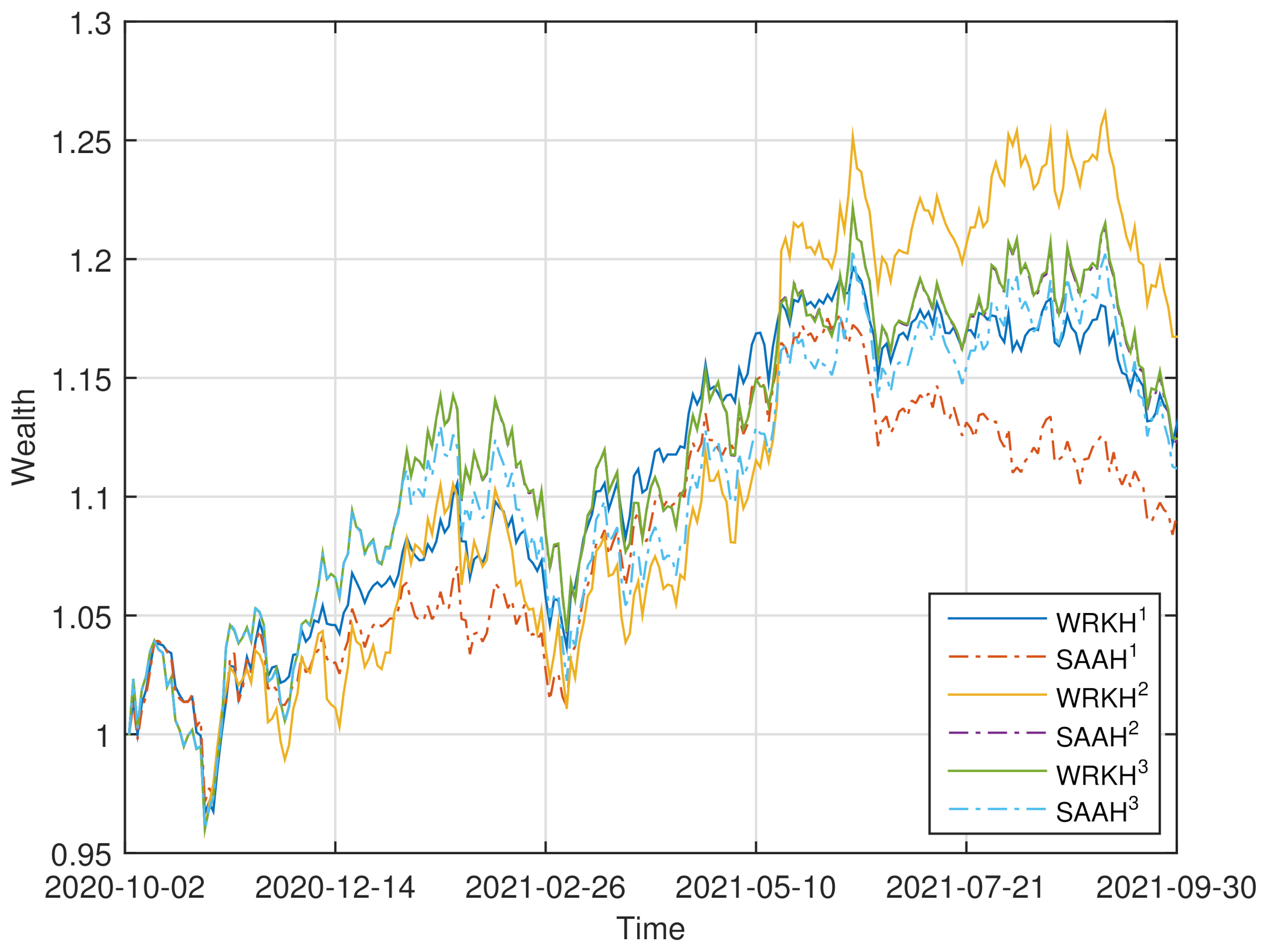
To demonstrate the effectiveness of “${\mathrm{WRKH}}^p,p=1,2,3$”, we conduct the rolling horizon experiment in a setting similar to that of [60]. The historical data of the asset returns in the previous T days is used to obtain the optimal portfolio weights by solving problem (32)–(34) and problems (30) with $p=1,2,3$. We then use the portfolio weights to compute the current portfolio returns by using the current asset returns. This process is continued by adding the returns data for the next period in the dataset and dropping the earliest returns data, until the end of the dataset is reached (see [40,60]). Comparisons with “${\mathrm{SAAH}}^p,p=1,2,3$” are also given by rolling horizon analysis. We set $T=500$, $\gamma =0.95$, ${\mathit{\lambda }}^0=(1/T)\mathbf{1}$, $\rho =10$ and $\tau =0.01$. For four datasets, the corresponding evolutions of the accumulated wealth of the six strategies (“${\mathrm{WRKH}}^p$” and “${\mathrm{SAAH}}^p$” with $p=1,2,3$) are plotted in Figure 1.

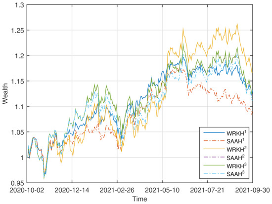
Figure 1. Wealth curves of “${\mathrm{WRKH}}^p$” and “${\mathrm{SAAH}}^p$” ($p=1,2,3$) for four datasets.

Four performance criteria are adopted to assess the quality of a portfolio selection strategy (see [40]): (i) the mean of the daily returns (denoted “MR”), (ii) the Sharpe ratio (denoted “SR”), (iii) the average turnover (denoted “TO”), (iv) the maximum drawdown (denoted “MDD”). The turnover indicates the volumes of rebalancing. There is no benefit for the portfolio strategies that yield a high turnover since a high “TO” incurs a high trading cost that reduces the portfolio return (see [35,60]). The maximum drawdown is an indicator of downside risk over a specified time period, which is the largest drop from a peak (see [61]). The performance, in the above four criteria, of the six strategies for four datasets is shown in Table 1. The better-performing strategy under different criteria is marked in bold fonts for $p=1,2,3$, respectively.

Table 1. Performance of “${\mathrm{WRKH}}^p$” and “${\mathrm{SAAH}}^p$” ($p=1,2,3$) for four datasets.

Dataset	Statistics	${\mathbf{WRKH}}^1$	${\mathbf{SAAH}}^1$	${\mathbf{WRKH}}^2$	${\mathbf{SAAH}}^2$	${\mathbf{WRKH}}^3$	${\mathbf{SAAH}}^3$
FF6	MR	0.001197	0.001090	0.000955	0.000927	0.001015	0.000938
	SR	0.1323	0.1235	0.1039	0.1015	0.1137	0.1028
	TO	0.0561	0.0395	0.2245	0	0.0367	0.0104
	MDD	0.0726	0.0727	0.0855	0.0858	0.0802	0.0858
FF30	MR	0.000576	0.000588	0.001435	0.001400	0.001366	0.001406
	SR	0.0807	0.0828	0.1540	0.1444	0.1466	0.1451
	TO	0.1855	0.0920	0.4710	0.1177	0.1319	0.1182
	MDD	0.0695	0.0690	0.0763	0.0835	0.0782	0.0838
FF48	MR	0.000471	0.000336	0.000672	0.000511	0.000515	0.000471
	SR	0.0646	0.0442	0.0649	0.0527	0.0533	0.0487
	TO	0.1466	0.0463	0.2731	0.0408	0.0408	0.1332
	MDD	0.0693	0.0822	0.0856	0.0873	0.0872	0.0950
FF100	MR	0.001349	0.001184	0.000350	0.000944	0.001003	0.000940
	SR	0.1442	0.1319	0.0221	0.0516	0.0981	0.0514
	TO	0.1663	0.0986	0.5570	0.0455	0.0359	0.0539
	MDD	0.0654	0.0697	0.2125	0.2482	0.0824	0.2482

From Figure 1 and Table 1, we can observe that: (i) For FF6, the wealthy curve of “${\mathrm{WRKH}}^1$” dominates those of the others most of the time. “MR”, “SR” and “MDD” of “${\mathrm{WRKH}}^p$” are better than those of “${\mathrm{SAAH}}^p$” for $p=1,2,3$, respectively. (ii) For FF30, the wealthy curves of “${\mathrm{WRKH}}^p,p=2,3$” overlaps with those of “${\mathrm{SAAH}}^p,p=2,3$”, and dominate those of “${\mathrm{WRKH}}^1$” and “${\mathrm{SAAH}}^1$” most of the time. “${\mathrm{WRKH}}^2$” has the optimal “MR” and “SR”. (iii) For FF48, the wealthy curve of “${\mathrm{WRKH}}^2$” overlaps with those of the others at the first half time, and dominates those of the others latter. “MR”, “SR” and “MDD” of “${\mathrm{WRKH}}^p$” are better than those of “${\mathrm{SAAH}}^p$” for $p=1,2,3$, respectively. (iv) For FF100, the wealthy curve of “${\mathrm{WRKH}}^1$” dominates those of the others most of the time. “MR”, “SR” and “MDD” of “${\mathrm{WRKH}}^p$” are better than those of “${\mathrm{SAAH}}^p$” for $p=1,3$, respectively.

3.2. Sensitivity Analysis

The numerical experiments of the sensitivity analysis of “${\mathrm{WRKH}}^p,p=1,2,3$” on $\tau$ and $\rho$ have also been conducted for FF30. There are similar results for the other datasets. The corresponding numerical results for FF30 are listed as follows.

Sensitivity on $\tau$. For $\tau =0.01,0.03,0.05,0.07,0.09$, the wealthy curves of “${\mathrm{WRKH}}^p,p=1,2,3$” with $\rho =10$ are shown in Figure 2a–c. The corresponding statistic of the performance of “${\mathrm{WRKH}}^p,p=1,2,3$” is shown in Table 2.

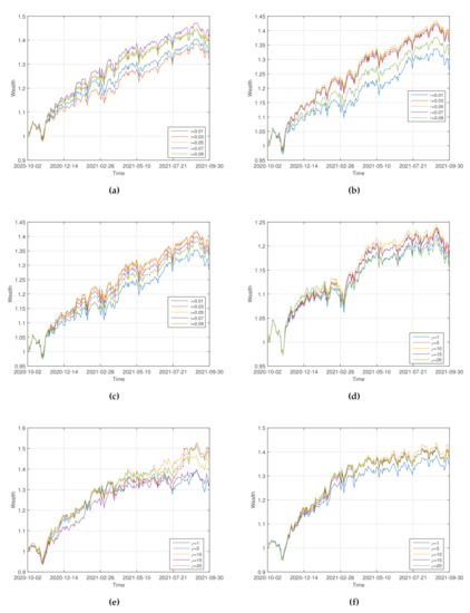
Figure 2. Wealth curves of “${\mathrm{WRKH}}^p,p=1,2,3$” for various values of $\tau$ (a–c) and $\rho$ (d–f).

Table 2. Sensitivity of “${\mathrm{WRKH}}^p,p=1,2,3$” on $\tau$.

p	Statistics	$\mathit{\tau }$
		0.01	0.03	0.05	0.07	0.09
1	MR	0.001197	0.001121	0.001335	0.001400	0.001301
	SR	0.1323	0.1270	0.1439	0.1501	0.1402
	TO	0.0561	0.0433	0.0925	0.0835	0.1046
	MDD	0.0726	0.0749	0.0693	0.0665	0.0707
2	MR	0.000955	0.001258	0.001283	0.001238	0.001098
	SR	0.1039	0.1415	0.1435	0.1390	0.1228
	TO	0.2245	0.0907	0.0676	0.0824	0.1359
	MDD	0.0855	0.0693	0.0684	0.0696	0.0779
3	MR	0.001016	0.001220	0.001236	0.001168	0.001115
	SR	0.1137	0.1380	0.1394	0.1322	0.1262
	TO	0.0367	0.0606	0.0577	0.0513	0.0451
	MDD	0.0802	0.0692	0.0691	0.0710	0.0748

From Figure 2a–c and Table 2, we can observe that: (i) For $p=2,3$, the wealthy curve of “$\tau =0.05$” dominates those of the others most of the time. “$\tau =0.05$” has the optimal “MR”, “SR” and “MDD”. (ii) For $p=1$, the wealthy curve of “$\tau =0.07$” dominates those of the others most of the time. “$\tau =0.07$” has the optimal “MR”, “SR” and “MDD”. It is suggested that for the good performance of “${\mathrm{WRKH}}^p,p=1,2,3$” the value of $\tau$ should not be too big or too small.

Sensitivity on $\rho$. For $\tau =1,5,10,15,20$, the wealthy curves of “${\mathrm{WRKH}}^p,p=1,2,3$” with $\tau =0.01$ are shown in Figure 2d–f. The corresponding statistic of the performance of “${\mathrm{WRKH}}^p,p=1,2,3$” is shown in Table 3.

Table 3. Sensitivity of “${\mathrm{WRKH}}^p,p=1,2,3$” on $\rho$.

p	Statistics	$\mathit{\rho }$
		1	5	10	15	20
1	MR	0.000593	0.000638	0.000670	0.000662	0.000576
	SR	0.0845	0.0905	0.0958	0.0945	0.0808
	TO	0.0587	0.1155	0.1583	0.1116	0.1855
	MDD	0.0703	0.0710	0.0698	0.0697	0.0695
2	MR	0.001126	0.001588	0.001435	0.001133	0.001512
	SR	0.1116	0.1509	0.1540	0.1212	0.1578
	TO	0.2883	0.6078	0.4710	0.5628	0.4568
	MDD	0.0809	0.0948	0.0763	0.0902	0.0704
3	MR	0.001204	0.001307	0.001366	0.001291	0.001300
	SR	0.1359	0.1400	0.1466	0.1415	0.1396
	TO	0.1263	0.1316	0.1319	0.1628	0.1417
	MDD	0.0710	0.0813	0.0782	0.0793	0.0818

From Figure 2d–f and Table 3, we can observe that: (i) For $p=1,3$, the wealthy curve of “$\rho =10$” dominates those of the others most of the time. “MR” and “SR” of “$\rho =10$” are optimal. (ii) For $p=2$, all wealthy curves are intertwined most of the time. “$\rho =5$” has the optimal “MR”, however “$\rho =20$” has the optimal “SR” and “MDD”. It is suggested from the numerical results that for the good performance of “${\mathrm{WRKH}}^p,p=1,2,3$” the risk aversion level $\rho$ should not be too big or too small.

4. Conclusions

We propose the Wasserstein distributionally robust portfolio optimization model based on a kernel smoothing method and mean-HMCR to solve three challenges arising from the asymmetry and nonlinearity of HMCR as well as the ambiguity of asset returns distribution. We obtain the tractable DCP reformulation of the corresponding DRO model. The experimental results show that our proposed model is promising. It remains open to calibrate KDE-Wasserstein radius $\tau$, which is left for future research.

References

- Wiesemann, W.; Kuhn, D.; Sim, M. Distributionally robust convex optimization. Oper. Res. 2014, 62, 1358–1376. [Google Scholar] [CrossRef] [Green Version]
- Knight, F.H. Risk, Uncertainty and Profit, 1st ed.; Hart, Schaffner and Marx: Boston, MA, USA, 1921. [Google Scholar]
- Markowitz, H. Portfolio selection. J. Financ. 1952, 7, 77–91. [Google Scholar]
- Krokhmal, P.A. Higher moment coherent risk measures. Quant. Financ. 2007, 7, 373–387. [Google Scholar] [CrossRef]
- Krokhmal, P.A.; Zabarankin, M.; Uryasev, S. Modeling and optimization of risk. Surv. Oper. Res. Manag. Sci. 2011, 16, 49–66. [Google Scholar] [CrossRef]
- Rockafellar, R.T.; Uryasev, S. Optimization of conditional value-at-risk. J. Risk 2000, 2, 21–42. [Google Scholar] [CrossRef] [Green Version]
- Artzner, P.; Delbaen, F.; Eber, J.M.; Heath, D. Coherent measures of risk. Math. Financ. 1999, 9, 203–228. [Google Scholar] [CrossRef]
- Fishburn, P.C. Mean-risk analysis with risk associated with below-target returns. Am. Econ. Rev. 1977, 67, 116–126. [Google Scholar]
- Rockafellar, R.T.; Uryasev, S.; Zabarankin, M. Generalized deviations in risk analysis. Financ. Stoch. 2006, 10, 51–74. [Google Scholar] [CrossRef]
- Fabozzi, F.J.; Huang, D.; Zhou, G. Robust portfolios: Contributions from operations research and finance. Ann. Oper. Res. 2010, 176, 191–220. [Google Scholar] [CrossRef] [Green Version]
- Shapiro, A.; Dentcheva, D.; Ruszczyński, A. Lectures on Stochastic Programming: Modeling and Theory, 2nd ed.; SIAM: Philadelphia, PA, USA, 2014. [Google Scholar]
- Ben-Tal, A.; Nemirovski, A. Robust Convex Optimization. Math. Oper. Res. 1998, 23, 769–805. [Google Scholar] [CrossRef] [Green Version]
- Ben-Tal, A.; El Ghaoui, L.; Nemirovski, A. Robust Optimization; Princeton University Press: Princeton, NJ, USA, 2009; Volume 28. [Google Scholar]
- Bertsimas, D.; Sim, M. The Price of Robustness. Oper. Res. 2004, 52, 35–53. [Google Scholar] [CrossRef] [Green Version]
- Scarf, H. A min-max solution of an inventory problem. In Studies in the Mathematical Theory of Inventory and Production; Scarf, H., Arrow, K., Karlin, S., Eds.; Stanford University Press: Stanford, CA, USA, 1958; Volume 10, pp. 201–209. [Google Scholar]
- El Ghaoui, L.; Oks, M.; Oustry, F. Worst-case value-at-risk and robust portfolio optimization: A conic programming approach. Oper. Res. 2003, 51, 543–556. [Google Scholar] [CrossRef] [Green Version]
- Bertsimas, D.; Popescu, I. Optimal Inequalities in Probability Theory: A Convex Optimization Approach. SIAM J. Optim. 2005, 15, 780–804. [Google Scholar] [CrossRef]
- Popescu, I. Robust mean-covariance solutions for stochastic optimization. Oper. Res. 2007, 55, 98–112. [Google Scholar] [CrossRef] [Green Version]
- Goh, J.; Sim, M. Distributionally robust optimization and its tractable approximations. Oper. Res. 2010, 58, 902–917. [Google Scholar] [CrossRef]
- Delage, E.; Ye, Y. Distributionally robust optimization under moment uncertainty with application to data-driven problems. Oper. Res. 2010, 58, 595–612. [Google Scholar] [CrossRef] [Green Version]
- Zymler, S.; Kuhn, D.; Rustem, B. Distributionally robust joint chance constraints with second-order moment information. Math. Program. 2013, 137, 167–198. [Google Scholar] [CrossRef] [Green Version]
- Hanasusanto, G.A.; Kuhn, D. Robust Data-Driven Dynamic Programming. In Advances in Neural Information Processing Systems 26; Burges, C.J.C., Bottou, L., Welling, M., Ghahramani, Z., Weinberger, K.Q., Eds.; Curran Associates, Inc.: Red Hook, NY, USA, 2013; pp. 827–835. Available online: https://proceedings.neurips.cc/paper/2013/hash/ef575e8837d065a1683c022d2077d342-Abstract.html (accessed on 15 October 2021).
- Erdoğan, E.; Iyengar, G. Ambiguous chance constrained problems and robust optimization. Math. Program. 2006, 107, 37–61. [Google Scholar] [CrossRef] [Green Version]
- Bertsimas, D.; Gupta, V.; Kallus, N. Robust sample average approximation. Math. Program. 2018, 171, 217–282. [Google Scholar] [CrossRef] [Green Version]
- Wang, Z.; Glynn, P.W.; Ye, Y. Likelihood robust optimization for data-driven problems. Comput. Manag. Sci. 2016, 13, 241–261. [Google Scholar] [CrossRef] [Green Version]
- Ben-Tal, A.; Den Hertog, D.; De Waegenaere, A.; Melenberg, B.; Rennen, G. Robust solutions of optimization problems affected by uncertain probabilities. Manag. Sci. 2013, 59, 341–357. [Google Scholar] [CrossRef] [Green Version]
- Bayraksan, G.; Love, D. Data-driven stochastic programming using phi-divergences. Tutor. Oper. Res. 2015, 1, 1–19. [Google Scholar]
- Jiang, R.; Guan, Y. Data-driven chance constrained stochastic program. Math. Program. 2016, 158, 291–327. [Google Scholar] [CrossRef]
- Shapiro, A. Distributionally robust stochastic programming. SIAM J. Optim. 2017, 27, 2258–2275. [Google Scholar] [CrossRef]
- Postek, K.; Hertog den, D.; Melenberg, B. Computationally tractable counterparts of distributionally robust constraints on risk measures. SIAM Rev. 2016, 58, 603–650. [Google Scholar] [CrossRef] [Green Version]
- Calafiore, G.C. Ambiguous risk measures and optimal robust portfolios. SIAM J. Optim. 2007, 18, 853–877. [Google Scholar] [CrossRef]
- Hu, Z.; Hong, L.J. Kullback-Leibler Divergence Constrained Distributionally Robust Optimization. 2012. Available online: http://www.optimization-online.org/DB_HTML/2012/11/3677.html (accessed on 15 October 2021).
- Mohajerin Esfahani, P.; Kuhn, D. Data-driven distributionally robust optimization using the Wasserstein metric: Performance guarantees and tractable reformulations. Math. Program. 2018, 171, 115–166. [Google Scholar] [CrossRef]
- Gao, R.; Kleywegt, A.J. Distributionally Robust Stochastic Optimization with Wasserstein Distance. arXiv 2016, arXiv:1604.02199v2. [Google Scholar]
- Wozabal, D. Robustifying convex risk measures for linear portfolios: A nonparametric approach. Oper. Res. 2014, 62, 1302–1315. [Google Scholar] [CrossRef]
- Zhao, C.; Guan, Y. Data-driven risk-averse stochastic optimization with Wasserstein metric. Oper. Res. Lett. 2018, 46, 262–267. [Google Scholar] [CrossRef]
- Mei, Y.; Chen, Z.P.; Ji, B.B.; Xu, Z.J.; Liu, J. Data-driven Stochastic Programming with Distributionally Robust Constraints Under Wasserstein Distance: Asymptotic Properties. J. Oper. Res. Soc. China 2021, 9, 525–542. [Google Scholar] [CrossRef]
- Nakagawa, K.; Ito, K. Taming Tail Risk: Regularized Multiple β Worst-Case CVaR Portfolio. Symmetry 2021, 13, 922. [Google Scholar] [CrossRef]
- Zhu, S.; Fukushima, M. Worst-case conditional value-at-risk with application to robust portfolio management. Oper. Res. 2009, 57, 1155–1168. [Google Scholar] [CrossRef]
- Liu, W.; Yang, L.; Yu, B. KDE distributionally robust portfolio optimization with higher moment coherent risk. Ann. Oper. Res. 2021, 307, 363–397. [Google Scholar] [CrossRef]
- Villani, C. Optimal Transport: Old and New; Springer: Berlin/Heidelberg, Germany, 2009. [Google Scholar]
- Silverman, B.W. Density Estimation for Statistics and Data Analysis, 2nd ed.; MPS-SIAM Series on Optimization; Chapman and Hall: New York, NY, USA, 1986. [Google Scholar]
- Li, Q.; Racine, J.S. Nonparametric Econometrics: Theory and Practice; Princeton University Press: Princeton, NJ, USA, 2007. [Google Scholar]
- Hazelton, M.L.; Turlach, B.A. Reweighted kernel density estimation. Comput. Stat. Data Anal. 2007, 51, 3057–3069. [Google Scholar] [CrossRef]
- Parzen, E. On estimation of a probability density function and mode. Ann. Math. Stat. 1962, 33, 1065–1076. [Google Scholar] [CrossRef]
- Terrell, G.R.; Scott, D.W. Variable Kernel Density Estimation. Ann. Stat. 1992, 20, 1236–1265. [Google Scholar] [CrossRef]
- Hall, P.; Minnotte, M.C. High order data sharpening for density estimation. J. R. Stat. Soc. Ser. B 2002, 64, 141–157. [Google Scholar] [CrossRef]
- Hall, P.; Turlach, B.A. Reducing bias in curve estimation by use of weights. Comput. Stat. Data Anal. 1999, 30, 67–86. [Google Scholar] [CrossRef]
- Owen, A.B. Empirical Likelihood; CRC Press: Boca Raton, FL, USA, 2001. [Google Scholar]
- Chen, S.X. Empilical likelihood-based kernel density estimation. Aust. J. Stat. 1997, 39, 47–56. [Google Scholar] [CrossRef]
- Rockafellar, R.T. Convex Analysis; Princeton University Press: Princeton, NJ, USA, 1997. [Google Scholar]
- Ben-Tal, A.; Den Hertog, D.; Vial, J.P. Deriving robust counterparts of nonlinear uncertain inequalities. Math. Program. 2015, 149, 265–299. [Google Scholar] [CrossRef]
- Boyd, S.; Kim, S.; Vandenberghe, L.; Hassibi, A. A tutorial on geometric programming. Optim. Eng. 2007, 8, 67–127. [Google Scholar] [CrossRef]
- Boyd, S.; Vandenberghe, L. Convex Optimization; Cambridge University Press: Cambridge, UK, 2004. [Google Scholar]
- Horst, R.; Thoai, N. DC Programming: Overview. J. Optim. Theory Appl. 1999, 103, 1–43. [Google Scholar] [CrossRef]
- Grant, M.; Boyd, S. CVX: Matlab Software for Disciplined Convex Programming, version 2.0 beta; September 2013. Available online: http://cvxr.com/cvx/citing/ (accessed on 15 October 2021).
- Lobo, M.S.; Vandenberghe, L.; Boyd, S.; Lebret, H. Applications of second-order cone programming. Linear Algebra Appl. 1998, 284, 193–228. [Google Scholar] [CrossRef] [Green Version]
- Izenman, A.J. Recent developments in nonparametric density estimation. J. Am. Stat. Assoc. 1991, 86, 205–224. [Google Scholar] [CrossRef]
- Jones, M.C.; Marron, J.S.; Sheather, S.J. A Brief Survey of Bandwidth Selection for Density Estimation. J. Am. Stat. Assoc. 1996, 91, 401–407. [Google Scholar] [CrossRef]
- DeMiguel, V.; Garlappi, L.; Uppal, R. Optimal versus naive diversification: How inefficient is the 1/N portfolio strategy? Rev. Financ. Stud. 2009, 22, 1915–1953. [Google Scholar] [CrossRef] [Green Version]
- Chekhlov, A.; Uryasev, S.; Zabarankin, M. Drawdown measure in portfolio optimization. Int. J. Theor. Appl. Financ. 2005, 8, 13–58. [Google Scholar] [CrossRef]
Publisher’s Note: MDPI stays neutral with regard to jurisdictional claims in published maps and institutional affiliations. |
© 2022 by the authors. Licensee MDPI, Basel, Switzerland. This article is an open access article distributed under the terms and conditions of the Creative Commons Attribution (CC BY) license (https://creativecommons.org/licenses/by/4.0/).