Abstract
In the real-world, symmetry or asymmetry widely exists in various problems. Some of them can be formulated as constrained multi-objective optimization problems (CMOPs). During the past few years, handling CMOPs by evolutionary algorithms has become more popular. Lots of constrained multi-objective optimization evolutionary algorithms (CMOEAs) have been proposed. Whereas different CMOEAs may be more suitable for different CMOPs, it is difficult to choose the best one for a CMOP at hand. In this paper, we propose an ensemble framework of CMOEAs that aims to achieve better versatility on handling diverse CMOPs. In the proposed framework, the hypervolume indicator is used to evaluate the performance of CMOEAs, and a decreasing mechanism is devised to delete the poorly performed CMOEAs and to gradually determine the most suitable CMOEA. A new CMOEA, namely ECMOEA, is developed based on the framework and three state-of-the-art CMOEAs. Experimental results on five benchmarks with totally 52 instances demonstrate the effectiveness of our approach. In addition, the superiority of ECMOEA is verified through comparisons to seven state-of-the-art CMOEAs. Moreover, the effectiveness of ECMOEA on the real-world problems is also evaluated for eight instances.
1. Introduction
Constrained multi-objective optimization problems (CMOPs) widely exist in real-world applications and scientific research fields, such as the multi-objective caching optimization [1], vehicle routing problems [2], web service location allocation problems [3], 3D indoor redeployment in IoT collection networks [4], asymmetric UAV trajectory planning [5], multi-objective testing resource allocation problems [6], and ring road bus lines and fare design [7]. Generally, CMOPs can be referred to as the optimization problems with constraints and two or more conflicting objectives [8], which can be mathematically formulated as:
where m denotes the number of objective functions, represents an n-dimensional decision vector, n denotes the number of decision variables, and are the search space. and are the i-th inequality and j-th equality constraints, respectively. q is the number of constraints.
The constraint violation () of at the j-th constraint can be formulated as:
where is a very small positive value to relax the equality constraints into inequality ones. The overall constraint violation (CV) of is formulated as:
is, feasible if ; otherwise, it is infeasible.
Due to the population-based feature, which accords to the requirement of a CMOP for a set of tradeoff solutions, and independence of prior knowledge or problem structure, evolutionary algorithms (EAs) are widely used in solving multi-objective optimization problems (MOPs) [9], many-objective optimization problems (MaOPs) [10] and CMOPs [11], for which we termed multi-objective optimization evolutionary algorithms (MOEAs), many-objective optimization evolutionary algorithms (MaOEAs) and constrained multi-objective optimization evolutionary algorithms (CMOEAs). They mainly include the dominance-based [12], decomposition-based [13] and indicator-based [14] ones. During the past two decades, lots of CMOEAs have been proposed [15,16,17], and the constrained multi-objective optimization (CMO) community has made great progress. However, despite the prosperity of CMO research field, these CMOEAs all have their own strengths and weaknesses [18]. For example, CCMO [17], which performs well on C-DTLZ [19] and DC-DTLZ [20] benchmarks, shows poor performance on LIR-CMOP [21] with large infeasible regions. On the contrary, PPS [22], which performs well on LIR-CMOP, fails to well handle C-DTLZ and DC-DTLZ.
According to the No Free Lunch theory, a CMOEA can not be effective for all kinds of CMOPs. That is to say, in face of the proposed CMOP benchmarks, a specific CMOEA can only handle one kind or several kinds of CMOPs. Designing a CMOEA which can adapt to all CMOPs is impossible. Given the fact that a CMOP in real-world situation may have different features and poses different challenges to CMOEA, enhancing the versatility of CMOEA is expected.
To overcome this drawback, in this paper, we propose an ensemble framework of CMOEAs, which aims to generate an adaptively selecting guided CMOEA filter to enhance the versatility of existing CMOEAs. The main contributions can be summarized as follows:
- An ensemble framework is proposed, into which any CMOEA can be easily embedded. The proposed framework can adaptively delete the poorly performed CMOEAs and gradually select the most suitable CMOEA for the CMOP to be solved.
- Three state-of-the-art CMOEAs (CCMO [17], ICMA [15] and PPS [22]) have been successfully embedded into the proposed framework and a new CMOEA termed ECMOEA is developed. Experimental results have demonstrated the effectiveness of the proposed framework.
- Experiments on five benchmarks and eight real-world applications have been conducted. Compared to seven state-of-the-art CMOEAs, ECMOEA achieved better or at least equal performance, which further demonstrated the effectiveness of the proposed framework, as well as ECMOEA.
The remainder of this article is organized as follows. Section 2 introduces the related work and motivations. Section 3 details the proposed framework and the generated ECMOEA, then gives the analysis. Afterwards, the experimental studies are presented in Section 4. Finally, some conclusions are drawn and future work is outlined in Section 5.
2. Related Work and Motivations
This section first presents a brief review and the taxonomy of the state-of-the-art CMOEAs. Then, the motivations are given.
2.1. State-of-the-Art CMOEAs
In order to achieve the constraint satisfaction, a constraint-handling technique (CHT) is necessary for a CMOEA. Based on the CHT adopted, the state-of-the-art CMOEAs can be roughly classified into the following three categories.
2.1.1. CMOEAs Based on Constrained Dominance Principle
The first category adopts constrained dominance principle (CDP) [12] as CHT. Assuming two solutions and , is said to constrained dominate (denoted as ), if one of the following conditions holds:
- ;
- and .
where means that dominates with both of the following conditions are satisfied:
- , ;
- , .
CDP is the most widely used CHT due to its simplicity on logic and implementation. Wang et al. [23] proposed a two phase based framework termed ToP in which a transformed constrained single objective optimization problem is optimized in the first phase and the original CMOP is optimized in the second phase. Yao et al. [20] proposed a two archive framework in which the convergence archive aims to promote convergence and feasibility while the diversity archive aims to promote diversity. Liu et al. [24] proposed a bidirectional coevolution framework in which one population approximates constrained Pareto front (CPF) from the feasible regions and the other from the infeasible regions. Tian et al. [17] proposed a weak coevolutionary framework in which one population solves the original CMOP while the other solves the constraints-ignored helper problem, and the two coevolved populations generate offspring on their own. Latter, Tian et al. [25] proposed an adaptively switched two stage framework in which one stage handles the original CMOP while the other ignores constraints. Wang et al. [18] proposed a two ranking based fitness evaluation mechanism in which CDP and Pareto dominance are both considered.
2.1.2. CMOEAs Based on -Constrained
The second category adopts constraint relaxation technique i.e., -constrained technique [26] as CHT. With the relaxation , some infeasible solutions might survive to the next generation. Therefore, it enhances the ability of the algorithm to jump out of local feasible regions. Specifically, for two solutions and , -constrained dominates (denoted as ), if one of the following conditions holds:
- and ;
- and ;
- and .
-constrained technique is also widely used in CMOP community since its relaxation of constraints can alleviate the shortages of CDP. Fan et al. [21] developed an update strategy of for the CMOPs with large infeasible regions. Then, they further did some research works on this topic in PPS [22] and PPS-M2M [27] by introducing new update strategies of . Zhang et al. [16] developed the detect-and-escape framework in which a detect strategy is designed to tell whether the search is trapped in local optimal and the escape strategy is designed to escape from the local optimal. Zeng et al. [28] proposed to transform a CMOP to a dynamic MOP and use an -constrained technique to handle constraints.
2.1.3. CMOEAs Based on Penalty Function
The third category adopts penalty function [29] as CHT. The penalty function combines the CV and objective function values to evaluate the fitness of a solution. Generally, the fitness of solution , , based on penalty function is calculated as
where is the penalty factor.
Jiao et al. [30] developed a feasible-guiding strategy to preserve some valuable infeasible solutions. In c-DPEA [31], Ming et al.designed a self-adaptive penalty function to preserve competitive infeasible solutions in one of its co-evolutionary populations. In ShiP [32], the positions of infeasible solutions are shifted, and the degree of shift is adaptively controlled by the feasible ratio in the current parent and offspring populations. Then, the shifted infeasible solutions are penalized based on the CV values. However, it is still a challenging task to adjust the penalty factor adaptively by using the population feedback information.
2.1.4. CMOEAs Based on New CHTs
Recently, some new CHTs have been proposed in the CMOP community. Some CMOEAs are also developed based on these new CHTs. Liu et al. [33] developed the indicator-based CMOEA framework, in which indicators are used to help with dealing with CMOPs. In TiGE-2 [34], a tri-goal technique is proposed in which three indicators are used for convergence, diversity and feasibility, respectively. Xiang et al. [35] proposed a new CHT which works for the CPF shape detection mechanism to detect problem type. Yuan et al. [15] proposed a new cost value based indicator of which the convergence to CPF property is proofed.
2.2. Motivations
2.2.1. The Limitation of Using a Single CMOEA
Although there have been many CMOEAs, the versatility of these methods is limited. According to the “No Free Lunch” theory, one single algorithm cannot effectively handle all kinds of problems. Different CMOEAs have different skills, which is to say, a specific CMOEA can only effectively handle one kind or some kinds of CMOPs. For example, the CMOEAs applying constraint relaxation technique (i.e., -constrained) are effective on CMOPs with complex infeasible regions since some infeasible solutions are expected for the algorithm to cross complex infeasible regions. On the contrary, ignoring constraints is effective on handling CMOPs whose PF is similar to or near CPF, because approaching PF can also approach CPF. To better understand this point, experiments of CCMO and PPS on DC2-DTLZ and LIR-CMOP2 are conducted. The parameter settings are the same to which in Section 4.1.3. It should be noted that CCMO is the one that ignores constraints in one of its coevolved populations while PPS is the one uses constraint relaxation technique. The results are presented in Figure 1. It can be easily seen that CCMO performed well on DC2-DTLZ1 (Figure 1a) but poorly on LIR-CMOP2 (Figure 1b), while PPS performed well on LIR-CMOP2 (Figure 1c) but poorly on DC2-DTLZ1 (Figure 1d).
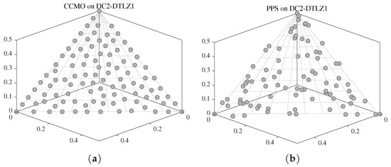
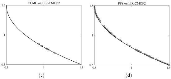
Figure 1.
Representative runs of two CMOEAs on two instances from two benchmarks. (a) CCMO on DC2-DTLZ1. (b) PPS on DC2-DTLZ1. (c) CCMO on LIR-CMOP2. (d) PPS on LIR-CMOP2.
2.2.2. Evaluating the Performance of a CMOEA by HV
Hypervolume (HV) [36] is a performance indicator used for evaluating the performance of an algorithm [37]. HV calculates the volume or hypervolume of the area surrounded by the obtained solution set and the reference point. Due to the independence of true CPF, HV is widely used in the CMOEA community for the performance evaluation when comparing a proposed approach to existing one, especially for real-world application problems whose true CPF is mostly unknown. Therefore, through the comparison of HV value, we can easily tell which CMOEA is better and which is worse. So in this paper, we propose to use HV as the selection criteria in designing the ensemble framework.
2.2.3. Ensemble of CMOEAs
As mentioned and analyzed above, one single CMOEA is not likely to be omnipotent for all kinds of CMOPs. Given the fact that there have been already many CMOEAs that can suit CMOPs with different features, developing an ensemble framework which can adaptively select the most effective CMOEA for a given CMOP is valuable. To be more specific, if an ensemble framework can integrate different CMOEAS such as CCMO and PPS, and tell which one can solve the current CMOP well, then, the ensemble obtains better versatility. In the next section, our proposed ensemble framework, as well as the generated ECMOEA, will be detailed.
3. Proposed Approach
3.1. The Proposed Ensemble Framework
The proposed ensemble framework of CMOEAs can be expressed as the flowchart shown in Figure 2. After initialization, the three embedded CMOEAs (denoted as CMOEA1, CMOEA2 and CMOEA3) are evolved simultaneously. Before (i.e., the first half of evolutionary process), all the three CMOEAs are evolved. When , the worst CMOEA is detected by comparing the HV values of the three CMOEAs’ populations. Then, the CMOEA with worst performance (i.e., HV value) is deleted. The evolution of the rest two CMOEAs (assume they are CMOEA1 and CMOEA2) are continued until . When , the worse CMOEA is detected through the comparison between their populations’ HV values. Then, the one with smaller HV value is deleted. Afterwards, the last survived CMOEA is evolved to the end of the evolutionary process. Finally, the population of the last CMOEA is output as the final solution set.
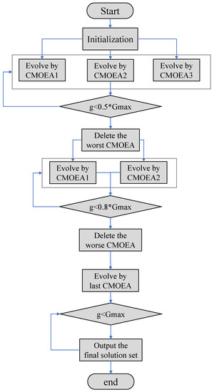
Figure 2.
The flowchart of the proposed ensemble framework.
Generally, the search process is divided into three stages. In the first stage (), all the CMOEAs embedded are evolved. In the second stage (), one CMOEA is deleted and the remained two are continued. In the third stage (), the last CMOEA is evolved to the end.
3.2. The Proposed ECMOEA
Based on the proposed ensemble framework as related in the above part, a new CMOEA termed ECMOEA is generated. In this paper, the generated ECMOEA is embedded with ICMA, CCMO and PPS. Specifically, these three state-of-the-art CMOEAs work as the CMOEA1, CMOEA2 and CMOEA3 in the framework. The pseudo code is shown in Algorithm 1. The details are as follows. Similarly, these three CMOEAs are denoted as CMOEA1, CMOEA2 and CMOEA3. Besides, the deleted CMEOAs are assumed to be CMOEA3 and CMOEA2 without losing generality.
| Algorithm 1 The Framework of ECMOEA |
| Input: N, termination condition () Output:
|
First of all, the populations and parameters (include the reference vector set if needed) are initialized (line 1). Furthermore, the determined mark and the generation index g are initialized (line 2). Then, until the termination condition met, the following steps are performed.
- If , lines 5–7 are performed, which is the first stage as mentioned above.
- If , lines 9–15 are performed, which is the second stage as mentioned above. The determined mark is used in this stage to determine whether the worst CMOEA is deleted.
- If , lines 18–26 are performed, which is the third stage as mentioned above. The determined mark is used in this stage to determine whether the worse CMOEA is deleted.
With ICMA, CCMO and PPS embedded, an instantiation is presented in Algorithm 2 to better understand the principle and procedure of the proposed framework, as well as the generated ECMOEA. In this example, without losing generality, we assume that ICMA is the most suitable CMOEA for the CMOP, while PPS is the most unsuitable CMOEA. Then the algorithm goes as follows:
First, three populations and all the parameters needed are initialized (lines 1–2). Then, in the first stage (lines 4–7), all the three CMOEAs are co-evolved to evolve , and , respectively. When , the HV values of , and are calculated. Since PPS is the most unsuitable CMOEA, is obtained the minimum HV value. Therefore, at the first decision time, PPS is deleted (lines 9–12).Then, since is set 1, during , ICMA and CCMO are co-evolved (lines 14–15). When , it comes to the second decision time (lines 18–21). Since ICMA is the most suitable CMOEA for the CMOP to be solved, the HV value of , obtained by CCMO, is less than the HV value of . Therefore, at this time, CCMO is deleted and in the rest evolutionary process, only ICMA is evolved (lines 22–23). Finally, , the population obtained by the most suitable CMOEA (i.e., ICMA) is regarded as the final solution set.
| Algorithm 2 The instantiation of ECMOEA |
| Input: N, termination condition () Output:
|
3.3. Computational Complexity
As mentioned above in this Section, ECMOEA mainly includes the embedded CMEOAs and the HV calculation. The computational complexity of the embedded CMOEAs are the same to the original CMOEAs. Since the calculation of HV values only performed at and , the time consumption can be ignored. Therefore, the computational complexity of the proposed ensemble framework is determined by the embedded CMOEAs. In this paper, since ICMA, CCMO and PPS are embedded, whose computational complexities are , and , the generated ECMOEA’s computational complexity is .
4. Experimental Results and Analysis
In this section, experimental studies are conducted on PlatEMO [38] matlab platform in order to evaluate the effectiveness of the proposed ensemble framework and the generated ECMOEA. Section 4.1 details the experimental settings, then, Section 4.2 demonstrates the effectiveness of the proposed ensemble framework. Section 4.3 presents the comparison results of ECMOEA to other methods and the analysis. Next, Section 4.4 evaluates the effectiveness of ECMOEA on real-world CMOPs. Finally, the effectiveness of ECMOEA on constrained many-objective optimization problems (CMaOPs) are tested in Section 4.5.
4.1. Experimental Settings
4.1.1. CMOEAs and CMOPs in Comparison
In the generated ECMOEA, ICMA [15], CCMO [17] and PPS [22] are embedded as the candidates. Therefore, these three CMOEAs are chosen as comparisons in Section 4.2. Besides, CMOEA-MS, C-TAEA, DCNSGA-III, MOEA/D-DAE, NSGA-II-ToR, TiGE-2 and ToP are chosen as comparisons in Section 4.3, Section 4.4 and Section 4.5.
In order to testify the effectiveness and versatility of the proposed framework and ECMOEA, five CMOP benchmarks are chosen. They are the DTLZ variants (i.e., C-DTLZ [12] and DC-DTLZ [20]), DAS-CMOP [39], FCP [15], LIR-CMOP [21] and MW [40]. The number of objectives m and decision variables n of each CMOP are set as follows. for all C-DTLZ and DC-DTLZ, as well as MW4, MW8, MW14, DAS-CMOP7-DAS-CMOP9 and LIR-CMOP13-14, while the rest of the CMOPs are all set . for C1-DTLZ1 as well as all the DC-DTLZ1 instances, and for the rest of C-DTLZ, DC-DTLZ. for MW, 30 for FCP, LIR-CMOP and DAS-CMOP.
4.1.2. Performance Indicators
The performance of a CMOEA is evaluated by two performance indicators: inverted generational distance (IGD) [10] and hypervolume (HV) [36]. IGD is calculated by Equation (5) when S is the final solution set, W is the reference vector set sampled on the true PF and is the Euclidean distance in the objective space between the solution in S and the vector in W:
Suppose is the Lebesgue measure, is the hypervolume shaped by the solution and the reference point, then HV is calculated by Equation (6):
A smaller IGD value means better performance of the algorithm. In contrast, the greater the HV value, the better the performance of the algorithm.
According to the approaches in [41], 10,000 uniformly distributed points were sampled on the true CPF for IGD calculation. As for the HV calculation, the objective values were first normalized, and in the normalized objective space, was adopted as the reference point for the HV calculation. Each algorithm was run independently 30 times on each test case. The mean and standard deviations of each metric (i.e., HV and IGD) were recorded. Then the Wilcoxon rank sum test [42] with a significance level of 0.05 and Friedman test [43] with Bonferroni correction at a significance level 0.05 were adopted to perform statistical analysis on the experimental results. In all the tables showing statistical results, we use “+”, “−”, and “=” to show that the result obtained by another CMOEA is significantly better, significantly worse or statistically similar to that obtained by ECMOEA.
4.1.3. Genetic Operators and Parameter Settings
PPS and MOEA/D-DAE adopt the DE operator since they are embedded with MOEA/D [13]. ToP also adopts DE as genetic operator. For these three methods, the parameter settings are , , , and . For ECMOEA and the other CMOEAs, Polynomial Mutation (PM) [12] and Simulated Binary Crossover (SBX) [44] are applied in the GA evolutionary operator with parameters set as follows.
- SBX: Crossover probability and distribution index .
- PM: Mutation probability and distribution index .
All other parameters for the MOEAs are the same as in their original literatures, which are the default settings in PlatEMO [38]. These parameter settings did not change in our experiments.
The population size N is set to 91 for all problems in the experiments. The maximum function evaluation times is set to 100,000 for C-DTLZ, DC-DTLZ, FCP and MW and 150,000 for DAS-CMOP and LIR-CMOP to ensure the convergence of these CMOP instances.
4.2. Demonstration of the Effectiveness of the Proposed Ensemble Framework
First of all, we designed the experiment to demonstrate the effectiveness of the proposed ensemble framework. Specifically, three state-of-the-art CMOEAS, ICMA, CCMO and PPS are embedded into the proposed framework, and a new CMOEA termed ECMOEA is generated as related above. Then, ECMOEA is compared with ICMA, CCMO and PPS in this part. Thus, the effectiveness of the proposed framework can be verified through comparison to its original implants.
The statistical results of ECMOEA and CCMO, ICMA, PPS on DAS-CMOP, DTLZ, FCP, LIR-CMOP and MW in terms of HV and IGD are reported in Table A1, Table A2, Table A3, Table A4, Table A5, Table A6, Table A7, Table A8, Table A9 and Table A10. Assuming and = mean the former CMOEA performed better than, worse than and equal to the latter one. From these tables we can see that:
- DAS-CMOP: ICMA > CCMO > PPS, while ICMA > CCMO > ECMOEA > PPS;
- DTLZ: CCMO > ICMA > PPS, while CCMO > ECMOEA > ICMA > PPS;
- FCP: ICMA > CCMO = PPS, while ECMOEA = ICMA > CCMO = PPS;
- LIR-CMOP: ICMA = PPS > CCMO, while ECMOEA > ICMA = PPS > CCMO;
- MW: ICMA > CCMO > PPS, while ICMA > CCMO = ECMOEA > PPS.
From these results, we can see that the most suitable CMOEA for DAS-CMOP, DTLZ, FCP, LIR-CMOP and MW are ICMA, CCMO, ICMA, ICMA (and PPS) and ICMA, respectively. Under the proposed framework, the generated ECMOEA finally obtained better results than those CMOEAs except for the most suitable one. This is because the evaluations are aparted to those worse CMOEAs, thus, ECMOEA can not concentrate on evolving the most suitable CMOEA. However, the results indicate that the proposed framework can finally select the suitable CMOEA.
4.3. Comparison to Other CMOEAs
Then, in this part, ECMOEA is compared with seven state-of-the-art CMOEAs: CMOEA-MS, C-TAEA, DCNSGA-III, MOEA/D-DAE, NSGA-II-ToR, TiGE-2 and ToP. The statistical results of ECMOEA and CMOEAs in comparison on DAS-CMOP, DTLZ, FCP, LIR-CMOP and MW in terms of HV and IGD are reported in Table A11, Table A12, Table A13, Table A14, Table A15, Table A16, Table A17, Table A18, Table A19 and Table A20, respectively. From the tables, the proposed ECMOEA obtained the best overall performance on DAS-CMOP, FCP, LIR-CMOP and MW benchmarks. As for DTLZ, ECMOEA was slightly worse than MOEA/D-DAE, but was better than other methods. Especially, ECMOEA performed well on FCP and LIE-CMOP benchmarks.
To better illustrate the results, the feasible and non-dominated solution sets obtained by ECMOEA on all DAS-CMOP, DTLZ, FCP, LIR-CMOP and MW instances with the median IGD value among 30 runs are depicted in Figure A1, Figure A2, Figure A3, Figure A4 and Figure A5. From these figures we can see ECMOEA can finally approximate CPF and obtain good distribution in face of the different features of these benchmarks. When dealing with DAS-CMOP with adjustable feasibility, convergence and diversity, the ensemble framework can select ICMA and CCMO to adapt to the requirements. When dealing with DTLZ with regular and irregular CPF, discontinuous feasible regions and inner-outer layer feasible regions, the weak coevoluion based CCMO can be selected to adapt to these features. When dealing with FCP, ICMA can be selected whose indicator-based CHT can preserve some infeasible solutions to better deal with FCP instances. Similarly, when dealing with LIR-CMOP, ICMA and PPS, which is tailored for LIR-CMOP, can be selected. When dealing with MW, which contains different geometric relations between PF and CPF, CCMO can be selected to adapt to the CMOPs whose CPF is close to PF, and ICMA or PPS can be selected when CPF is far from PF.
The KEEL [45] software was used to perform the non-parameter statistical analysis on HV and IGD results. The Friedman test and the Wilcoxon test were conducted. The results of Friedman test are reported in Table 1, where the grey-blodface indicates the best ranking obtained by an algorithm and the blodface means the second ranking of an algorithm. As we can see, ECMOEA obtained the first ranking, while ICMA and CCMO obtained the second and the third, respectively. The results of Wilcoxon test are reported in Table 2 and Table 3, respectively. As can be seen, ECMOEA was significantly better than other all methods. Therefore, ECMOEA outperformed other methods statistically.

Table 1.
Average rankings of HV and IGD by Friedman test for ECMOEA and CMOEAs in comparison.
Table 2.
Summary of the Wilcoxon test on HV indicator. Hereinafter, • = the method in the row improves the method of the column, ◦ = the method in the column improves the method of the row. Upper diagonal of level significance , Lower diagonal level of significance .
Table 3.
Summary of the Wilcoxon test on IGD indicator.
4.4. ECMOEA on Real-World CMOPs
In this part, experiments of ECMOEA and CMOEAs in comparison on eight mechanical and chemical applications from RWMOP [46] are performed. The detailed parameter settings and information about these real-world CMOPs are shown in Table 4. The original references can be found in RWMOP literature.
Table 4.
Parameter settings for ECMOEA and CMOEAs in comparison on real-world application problems, where m is the number of objective functions, n is the number of decision variables, N is the population size and is the maximum number of function evaluations.
Since the true CPF of these real-world CMOPs are unknown, only HV is used for the comparison of ECMOEA and other methods. The statistical results of HV obtained by ECMOEA and CMOEAs in comparison on these eight instances are reported in Table A21. It is clear that ECMOEA obtained the best overall results on all the eight instances. ECMOEA outperformed most other methods when dealing with various real-world problems with various features. This is because ECMOEA can adapt to different problems with the help of the ensemble framework.
Two bar truss design (TBT) problem is chosen for further studies. The mathematical formulations of objective functions and constraints are as follows:
The feasible and non-dominated solution sets obtained by ECMOEA and other methods on TBT with the median IGD value among 30 runs are presented in Figure A6. From the results we can find that ECMOEA finally approximated CPF and obtained good distribution.
4.5. ECMOEA on CMaOPs
In this part, the effectiveness of ECMOEA on CMaOPs is tested through comparisons on C-DTLZ and DC-DTLZ test suites. For , for C1-DTLZ1 and DC1-DTLZ1, for other instances, the population size is and the maximum evaluation is 100,000, 140,000, respectively. The experimental settings are the same to which introduced in Section 4.1.
The statistical results on HV and IGD are listed in Table A22 and Table A23, respectively. Generally, ECMOEA obtained slightly better overall performance than ICMA, CCMO and PPS. The reasons can be that, since three CMOEAs (i.e., ICMA, CCMO and PPS) are all co-evolved during the evolutionary process, the function evaluations are divided. Therefore, in dealing with some CMOPs that the embedded CMOEA is good at (e.g., ICMA and CCMO on C-DTLZ), even ECMOEA finally find the most suitable CMOEA, less evaluations are used. On the contrary, ECMOEA can outperform ICMA and CCMO on some DC-DTLZ instances, because ECMOEA finally found that PPS is more suitable for these DC-DTLZ instances as DC-DTLZ instances are of more complex infeasible regions.
However, the other algorithms, especially the constrained many-objective optimization evolutionary algorithms (CMaOEAs) in comparison, obtained better performance than ECMOEA.
5. Conclusions
In this paper, an ensemble framework of CMOEA is proposed, into which any existing CMOEA or new CMOEA can be easily embedded. The framework possesses the ability to tell which CMOEA is the best for the given CMOP, and thus, choosing the most suitable CMOEA as the solver. Based on this ensemble framework and three state-of-the-art CMOEAs, a new CMOEA termed ECMOEA is proposed. The proposed ECMOEA can gradually delete the poorly performed CMOEAs and finally choose the most suitable one.
Experimental results on five benchmarks of totally 52 instances have verified the effectiveness of the proposed framework, and demonstrated the superiority or at least competitiveness of ECMOEA compared to seven state-of-the-art CMOEAs. Furthermore, the effectiveness of ECMOEA on real-world applications have been testified through experiments on eight real-world application CMOPs.
In the future, the following attempts are worth trying:
- Embedding other CMOEAs or mathematical methods into the framework to further enhance the versatility of ECMOEA;
- Designing an adaptive strategy instead of the current 0.8, 0.5 strategy can save the evaluations for the most suitable CMOEA;
- Adopting advanced techniques in Machine learning field such as the k-nearest neighbors algorithm (KNN) [47] to improve the efficiency of the ensemble framework is also worth trying;
- Embedding effective CMaOEAs in the ensemble framework to enhance the performance on handling CMaOPs is also expected.
Author Contributions
Conceptualization, methodology, validation, data curation, writing—original draft preparation, J.K.; validation, data curation, writing—original draft preparation, F.M.; supervision, writing—review and editing, funding acquisition, W.G. All authors have read and agreed to the published version of the manuscript.
Funding
This work was partly supported by the Hainan Provincial Natural Science Foundation of China under Grant No. 621RC599 and the National Natural Science Foundation of China under Grant No. 62076225.
Institutional Review Board Statement
Not applicable.
Informed Consent Statement
Not applicable.
Data Availability Statement
Not applicable.
Conflicts of Interest
The authors declare no conflict of interest.
Abbreviations
The following abbreviations are used in this manuscript:
| CMOPs | Constrained multi-objective optimization problems |
| CMOEAs | Constrained multi-objective optimization evolutionary algorithms |
| HV | Hypervolume |
| ECMOEA | Ensemble of constrained multi-objective optimization evolutionary algorithm |
| CMO | Constrained multi-objective optimization |
| MaOEAs | Many-objective optimization evolutionary algorithms |
| MOPs | Multi-objective optimization problems |
| CHT | Constraint-handling technique |
| CDP | Constrained dominance principle |
| CPF | Constrained Pareto front |
Appendix A
Table A1.
Statistical results of HV obtained by ECMOEA and CMOEAs embedded on DAS-CMOP benchmark problems. Best result in each row is highlighted.
Table A1.
Statistical results of HV obtained by ECMOEA and CMOEAs embedded on DAS-CMOP benchmark problems. Best result in each row is highlighted.
| Problem | CCMO | ICMA | PPS | ECMOEA |
|---|---|---|---|---|
| DASCMOP1 | 1.0955 × (1.22 × ) − | 2.1186 × (4.66 × ) ≈ | 1.8005 × (4.64 × ) − | 2.1202 × (4.62 × ) |
| DASCMOP2 | 2.5804 × (2.26 × ) − | 3.5513 × (7.10 × ) + | 3.5448 × (1.09 × ) − | 3.5504 × (7.11 × ) |
| DASCMOP3 | 2.1644 × (1.65 × ) − | 3.1169 × (6.35 × ) ≈ | 2.2181 × (3.19 × ) − | 3.1191 × (4.13 × ) |
| DASCMOP4 | 2.0215 × (3.58 × ) + | 1.7537 × (4.37 × ) ≈ | 1.3695 × (5.84 × ) − | 1.7485 × (4.48 × ) |
| DASCMOP5 | 3.5138 × (1.26 × ) + | 3.2192 × (6.86 × ) − | 2.9023 × (1.09 × ) − | 3.3874 × (4.35 × ) |
| DASCMOP6 | 3.0330 × (1.16 × ) + | 2.0688 × (1.05 × ) ≈ | 1.5702 × (1.29 × ) − | 2.4548 × (9.70 × ) |
| DASCMOP7 | 2.8808 × (3.28 × ) + | 2.7977 × (1.49 × ) + | 1.9470 × (1.01 × ) − | 2.7886 × (1.84 × ) |
| DASCMOP8 | 2.0676 × (4.33 × ) + | 2.0230 × (1.18 × ) ≈ | 1.5235 × (5.44 × ) − | 1.9989 × (1.74 × ) |
| DASCMOP9 | 1.2726 × (1.13 × ) − | 2.0623 × (2.37 × ) + | 1.5957 × (3.86 × ) − | 2.0613 × (2.33 × ) |
| × | 5/4/0 | 3/1/5 | 0/9/0 |
Table A2.
Statistical results of IGD obtained by ECMOEA and CMOEAs embedded on DAS-CMOP benchmark problems. Best result in each row is highlighted.
Table A2.
Statistical results of IGD obtained by ECMOEA and CMOEAs embedded on DAS-CMOP benchmark problems. Best result in each row is highlighted.
| Problem | CCMO | ICMA | PPS | ECMOEA |
|---|---|---|---|---|
| DASCMOP1 | 7.1644 × (3.65 × ) − | 3.5170 × (2.94 × ) + | 1.4262 × (2.25 × ) − | 3.9235 × (5.39 × ) |
| DASCMOP2 | 2.4445 × (2.81 × ) − | 4.6777 × (1.14 × ) + | 5.7132 × (1.86 × ) − | 4.7686 × (1.02 × ) |
| DASCMOP3 | 3.2465 × (3.87 × ) − | 2.0115 × (4.85 × ) ≈ | 3.0145 × (1.01 × ) − | 1.9721 × (1.18 × ) |
| DASCMOP4 | 1.9585 × (1.23 × ) + | 8.0629 × (1.15 × ) ≈ | 2.4094 × (2.22 × ) − | 7.8203 × (1.17 × ) |
| DASCMOP5 | 3.0351 × (8.18 × ) + | 4.9244 × (1.11 × ) − | 1.1761 × (2.20 × ) − | 2.2552 × (6.96 × ) |
| DASCMOP6 | 3.3377 × (2.57 × ) + | 2.1590 × (1.90 × ) ≈ | 3.7859 × (3.15 × ) − | 1.5724 × (2.12 × ) |
| DASCMOP7 | 3.1554 × (6.02 × ) + | 4.7193 × (2.93 × ) + | 2.7692 × (3.05 × ) − | 5.0821 × (3.96 × ) |
| DASCMOP8 | 4.1461 × (7.30 × ) + | 5.0302 × (2.08 × ) + | 2.1402 × (1.74 × ) − | 5.5965 × (3.30 × ) |
| DASCMOP9 | 3.7207 × (6.85 × ) − | 4.2816 × (7.71 × ) ≈ | 2.3194 × (1.65 × ) − | 4.3039 × (8.96 × ) |
| × | 5/4/0 | 4/1/4 | 0/9/0 |
Table A3.
Statistical results of HV obtained by ECMOEA and CMOEAs embedded on DTLZ benchmark problems. Best result in each row is highlighted.
Table A3.
Statistical results of HV obtained by ECMOEA and CMOEAs embedded on DTLZ benchmark problems. Best result in each row is highlighted.
| Problem | CCMO | ICMA | PPS | ECMOEA |
|---|---|---|---|---|
| C1-DTLZ1 | 8.3793 × (4.15 × ) + | 8.3640 × (9.53 × ) ≈ | 8.1831 × (4.15 × ) − | 8.3117 × (9.67 × ) |
| C1-DTLZ3 | 5.5756 × (1.45 × ) ≈ | 3.1578 × (2.27 × ) − | 2.8246 × (2.54 × ) − | 5.5559 × (6.92 × ) |
| C2-DTLZ2 | 5.1357 × (1.66 × ) ≈ | 5.0529 × (2.24 × ) − | 4.9844 × (3.73 × ) − | 5.1346 × (1.64 × ) |
| C3-DTLZ4 | 7.7982 × (4.59 × ) − | 7.9037 × (9.15 × ) ≈ | 7.6121 × (2.65 × ) − | 7.9059 × (8.34 × ) |
| DC1-DTLZ1 | 6.3124 × (1.32 × ) + | 6.2189 × (2.72 × ) − | 5.6239 × (7.39 × ) − | 6.3048 × (1.77 × ) |
| DC1-DTLZ3 | 4.7277 × (1.12 × ) + | 3.5011 × (1.26 × ) − | 2.9593 × (1.42 × ) − | 4.6722 × (2.48 × ) |
| DC2-DTLZ1 | 8.4029 × (6.69 × ) + | 6.8184 × (1.90 × ) − | 7.4682 × (1.44 × ) − | 8.1760 × (7.45 × ) |
| DC2-DTLZ3 | 5.5765 × (1.30 × ) + | 8.6141 × (4.27 × ) − | 1.6481 × (2.40 × ) − | 4.4170 × (1.82 × ) |
| DC3-DTLZ1 | 5.3493 × (1.36 × ) ≈ | 4.4580 × (1.66 × ) − | 1.3712 × (1.95 × ) − | 5.3397 × (2.92 × ) |
| DC3-DTLZ3 | 3.6618 × (1.62 × ) + | 0.0000 × (0.00 × ) − | 1.5702 × (6.49 × ) − | 1.8319 × (1.59 × ) |
| × | 6/1/3 | 0/8/2 | 0/10/0 |
Table A4.
Statistical results of IGD obtained by ECMOEA and CMOEAs embedded on DTLZ benchmark problems. Best result in each row is highlighted.
Table A4.
Statistical results of IGD obtained by ECMOEA and CMOEAs embedded on DTLZ benchmark problems. Best result in each row is highlighted.
| Problem | CCMO | ICMA | PPS | ECMOEA |
|---|---|---|---|---|
| C1-DTLZ1 | 2.1026 × (2.08 × ) + | 2.2331 × (3.27 × ) ≈ | 2.5579 × (6.00 × ) − | 2.2863 × (2.55 × ) |
| C1-DTLZ3 | 5.6293 × (7.47 × ) ≈ | 2.6582 × (2.64 × ) − | 3.5246 × (4.00 × ) − | 5.7235 × (3.87 × ) |
| C2-DTLZ2 | 4.5218 × (7.21 × ) ≈ | 4.8490 × (7.42 × ) − | 5.5625 × (1.91 × ) − | 4.4994 × (4.98 × ) |
| C3-DTLZ4 | 1.2440 × (1.35 × ) − | 1.0368 × (1.25 × ) − | 1.6846 × (9.08 × ) − | 1.0285 × (1.51 × ) |
| DC1-DTLZ1 | 1.2128 × (1.30 × ) ≈ | 1.2549 × (2.18 × ) − | 4.2156 × (5.79 × ) − | 1.2178 × (1.84 × ) |
| DC1-DTLZ3 | 3.5809 × (4.23 × ) ≈ | 9.8393 × (8.14 × ) − | 5.0327 × (7.73 × ) − | 4.6968 × (6.10 × ) |
| DC2-DTLZ1 | 2.1196 × (1.21 × ) + | 8.3092 × (7.43 × ) − | 5.2025 × (5.43 × ) − | 2.8151 × (2.73 × ) |
| DC2-DTLZ3 | 5.5824 × (6.52 × ) + | 6.0923 × (9.23 × ) − | 4.2698 × (2.40 × ) − | 1.4449 × (1.73 × ) |
| DC3-DTLZ1 | 7.2739 × (9.68 × ) ≈ | 3.5131 × (6.28 × ) − | 8.8632 × (1.39 × ) − | 7.3281 × (1.26 × ) |
| DC3-DTLZ3 | 2.1295 × (3.42 × ) + | 1.3236 × (6.04 × ) − | 3.4857 × (2.53 × ) − | 2.6746 × (2.54 × ) |
| × | 4/1/5 | 0/9/1 | 0/10/0 |
Table A5.
Statistical results of HV obtained by ECMOEA and CMOEAs embedded on FCP benchmark problems. Best result in each row is highlighted.
Table A5.
Statistical results of HV obtained by ECMOEA and CMOEAs embedded on FCP benchmark problems. Best result in each row is highlighted.
| Problem | CCMO | ICMA | PPS | ECMOEA |
|---|---|---|---|---|
| FCP1 | NaN (NaN) | 5.8083 × (1.86 × ) ≈ | NaN (NaN) | 5.8083 × (1.37 × ) |
| FCP2 | NaN (NaN) | 4.3108 × (3.92 × ) ≈ | NaN (NaN) | 4.3120 × (1.92 × ) |
| FCP3 | NaN (NaN) | 3.4654 × (6.65 × ) ≈ | NaN (NaN) | 3.4653 × (1.48 × ) |
| FCP4 | NaN (NaN) | 6.3374 × (3.75 × ) ≈ | NaN (NaN) | 6.3374 × (4.57 × ) |
| FCP5 | 2.4812 × (5.29 × ) − | 4.4573 × (7.36 × ) ≈ | 2.5936 × (6.08 × ) − | 4.2380 × (9.07 × ) |
| × | 0/1/0 | 0/0/5 | 0/1/0 |
Table A6.
Statistical results of IGD obtained by ECMOEA and CMOEAs embedded on FCP benchmark problems. Best result in each row is highlighted.
Table A6.
Statistical results of IGD obtained by ECMOEA and CMOEAs embedded on FCP benchmark problems. Best result in each row is highlighted.
| Problem | CCMO | ICMA | PPS | ECMOEA |
|---|---|---|---|---|
| FCP1 | NaN (NaN) | 3.9157 × (1.10 × ) ≈ | NaN (NaN) | 3.9006 × (7.10 × ) |
| FCP2 | NaN (NaN) | 3.9626 × (7.77 × ) ≈ | NaN (NaN) | 3.9383 × (1.03 × ) |
| FCP3 | NaN (NaN) | 4.3004 × (8.80 × ) ≈ | NaN (NaN) | 4.2828 × (1.24 × ) |
| FCP4 | NaN (NaN) | 3.0491 × (9.80 × ) ≈ | NaN (NaN) | 3.0694 × (1.50 × ) |
| FCP5 | 4.6497 × (1.07 × ) − | 6.4384 × (1.61 × ) ≈ | 4.6815 × (9.93 × ) − | 1.1119 × (2.00 × ) |
| × | 0/1/0 | 0/0/5 | 0/1/0 |
Table A7.
Statistical results of HV obtained by ECMOEA and CMOEAs embedded on LIR-CMOP benchmark problems. Best result in each row is highlighted.
Table A7.
Statistical results of HV obtained by ECMOEA and CMOEAs embedded on LIR-CMOP benchmark problems. Best result in each row is highlighted.
| Problem | CCMO | ICMA | PPS | ECMOEA |
|---|---|---|---|---|
| LIRCMOP1 | 1.2872 × (2.27 × ) − | 2.1268 × (1.43 × ) − | 2.2550 × (1.34 × ) ≈ | 2.2184 × (1.41 × ) |
| LIRCMOP2 | 2.4237 × (2.01 × ) − | 3.4296 × (6.18 × ) − | 3.4994 × (1.70 × ) − | 3.5079 × (7.94 × ) |
| LIRCMOP3 | 1.1113 × (1.66 × ) − | 1.8126 × (1.57 × ) − | 1.7366 × (2.83 × ) ≈ | 1.8854 × (1.36 × ) |
| LIRCMOP4 | 2.0371 × (2.15 × ) − | 2.8076 × (1.46 × ) − | 2.8100 × (3.20 × ) ≈ | 2.8486 × (2.73 × ) |
| LIRCMOP5 | 1.6274 × (2.75 × ) − | 1.8179 × (1.08 × ) − | 2.8046 × (5.30 × ) ≈ | 2.8993 × (1.09 × ) |
| LIRCMOP6 | 1.1719 × (1.44 × ) − | 1.3177 × (6.56 × ) − | 1.9630 × (2.74 × ) + | 1.9391 × (6.44 × ) |
| LIRCMOP7 | 2.4807 × (8.05 × ) − | 2.8512 × (1.33 × ) + | 2.4584 × (1.27 × ) − | 2.7155 × (1.91 × ) |
| LIRCMOP8 | 2.3460 × (1.16 × ) − | 2.9214 × (6.83 × ) ≈ | 2.3764 × (2.03 × ) − | 2.8425 × (1.70 × ) |
| LIRCMOP9 | 3.5952 × (6.03 × ) − | 4.8875 × (3.01 × ) ≈ | 4.1392 × (6.41 × ) − | 4.7741 × (2.89 × ) |
| LIRCMOP10 | 6.3190 × (3.18 × ) − | 6.9252 × (2.70 × ) + | 5.7897 × (6.37 × ) − | 6.7585 × (3.22 × ) |
| LIRCMOP11 | 6.6408 × (1.49 × ) − | 6.7655 × (2.98 × ) ≈ | 4.7948 × (1.44 × ) − | 6.7327 × (2.91 × ) |
| LIRCMOP12 | 5.0812 × (4.95 × ) − | 5.8038 × (1.99 × ) ≈ | 5.1359 × (4.81 × ) − | 5.8864 × (2.42 × ) |
| LIRCMOP13 | 5.5146 × (1.50 × ) ≈ | 5.4305 × (1.52 × ) − | 5.0949 × (6.83 × ) − | 5.5170 × (1.14 × ) |
| LIRCMOP14 | 5.5160 × (1.31 × ) ≈ | 5.5067 × (1.37 × ) ≈ | 5.2900 × (4.89 × ) − | 5.5091 × (1.62 × ) |
| × | 0/12/2 | 2/7/5 | 1/9/4 |
Table A8.
Statistical results of IGD obtained by ECMOEA and CMOEAs embedded on LIR-CMOP benchmark problems. Best result in each row is highlighted.
Table A8.
Statistical results of IGD obtained by ECMOEA and CMOEAs embedded on LIR-CMOP benchmark problems. Best result in each row is highlighted.
| Problem | CCMO | ICMA | PPS | ECMOEA |
|---|---|---|---|---|
| LIRCMOP1 | 2.5203 × (7.52 × ) − | 6.6140 × (4.37 × ) − | 3.0230 × (2.54 × ) ≈ | 4.0024 × (3.57 × ) |
| LIRCMOP2 | 2.3703 × (3.69 × ) − | 3.7748 × (1.13 × ) − | 2.3535 × (2.66 × ) + | 2.5367 × (1.84 × ) |
| LIRCMOP3 | 2.7298 × (5.77 × ) − | 7.0818 × (3.72 × ) − | 8.5862 × (7.58 × ) ≈ | 4.8873 × (3.63 × ) |
| LIRCMOP4 | 2.6501 × (4.89 × ) − | 8.2278 × (4.35 × ) ≈ | 8.1263 × (7.43 × ) ≈ | 7.1909 × (5.97 × ) |
| LIRCMOP5 | 2.8041 × (7.01 × ) − | 3.8995 × (4.33 × ) − | 4.8833 × (2.19 × ) ≈ | 9.0963 × (1.35 × ) |
| LIRCMOP6 | 2.8170 × (8.78 × ) − | 3.2398 × (3.75 × ) − | 8.5503 × (9.04 × ) + | 1.5276 × (2.00 × ) |
| LIRCMOP7 | 1.1862 × (2.65 × ) − | 2.7066 × (2.98 × ) + | 1.2701 × (3.44 × ) − | 5.9428 × (4.55 × ) |
| LIRCMOP8 | 1.8640 × (5.22 × ) − | 1.2245 × (1.39 × ) ≈ | 1.7233 × (6.74 × ) − | 3.2441 × (4.54 × ) |
| LIRCMOP9 | 4.9733 × (1.40 × ) − | 2.1397 × (9.56 × ) ≈ | 4.2851 × (1.04 × ) − | 2.2752 × (8.98 × ) |
| LIRCMOP10 | 1.3175 × (6.23 × ) − | 3.4225 × (6.06 × ) + | 2.6110 × (1.13 × ) − | 7.4373 × (7.04 × ) |
| LIRCMOP11 | 6.6407 × (3.89 × ) − | 3.2105 × (4.79 × ) ≈ | 3.2091 × (1.99 × ) − | 3.8158 × (4.76 × ) |
| LIRCMOP12 | 2.3432 × (9.48 × ) − | 9.2714 × (4.22 × ) ≈ | 2.1935 × (9.31 × ) − | 7.4168 × (5.49 × ) |
| LIRCMOP13 | 9.8279 × (1.05 × ) ≈ | 1.0697 × (1.72 × ) − | 1.2826 × (3.72 × ) − | 9.8540 × (1.15 × ) |
| LIRCMOP14 | 1.0055 × (1.11 × ) + | 1.0661 × (1.53 × ) − | 1.1993 × (3.18 × ) − | 1.0417 × (3.49 × ) |
| × | 1/12/1 | 2/7/5 | 2/8/4 |
Table A9.
Statistical results of HV obtained by ECMOEA and CMOEAs embedded on MW benchmark problems. Best result in each row is highlighted.
Table A9.
Statistical results of HV obtained by ECMOEA and CMOEAs embedded on MW benchmark problems. Best result in each row is highlighted.
| Problem | CCMO | ICMA | PPS | ECMOEA |
|---|---|---|---|---|
| MW1 | 4.8992 × (6.89 × ) + | 4.8826 × (3.86 × ) − | 4.8420 × (2.69 × ) − | 4.8916 × (1.48 × ) |
| MW2 | 5.5049 × (1.05 × ) − | 5.7928 × (1.81 × ) + | 3.9366 × (8.32 × ) − | 5.7126 × (1.07 × ) |
| MW3 | 5.4384 × (6.38 × ) − | 5.4437 × (3.89 × ) + | 5.4280 × (5.84 × ) − | 5.4418 × (2.99 × ) |
| MW4 | 8.3987 × (4.03 × ) + | 8.3380 × (9.96 × ) + | 8.0586 × (8.67 × ) − | 8.2426 × (1.76 × ) |
| MW5 | 3.2352 × (1.23 × ) + | 3.2030 × (1.09 × ) + | 2.0772 × (1.11 × ) − | 3.1721 × (4.36 × ) |
| MW6 | 2.9419 × (3.62 × ) − | 3.2486 × (3.09 × ) + | 1.2218 × (1.03 × ) − | 3.1025 × (1.47 × ) |
| MW7 | 4.1210 × (3.76 × ) ≈ | 4.1098 × (6.43 × ) − | 4.1124 × (4.36 × ) − | 4.1184 × (5.86 × ) |
| MW8 | 5.2782 × (1.76 × ) ≈ | 5.1042 × (1.18 × ) − | 3.5888 × (9.51 × ) − | 5.2682 × (1.40 × ) |
| MW9 | 3.8511 × (7.28 × ) + | 3.9409 × (1.62 × ) + | 3.1711 × (1.29 × ) − | 3.8030 × (5.76 × ) |
| MW10 | 4.1229 × (1.86 × ) ≈ | 4.4776 × (6.45 × ) + | 2.2396 × (1.10 × ) − | 4.1951 × (1.84 × ) |
| MW11 | 4.4633 × (2.31 × ) ≈ | 4.4703 × (3.13 × ) ≈ | 4.4720 × (1.86 × ) + | 4.4708 × (2.65 × ) |
| MW12 | 6.0426 × (4.06 × ) + | 6.0387 × (2.28 × ) ≈ | 5.2215 × (1.68 × ) − | 6.0390 × (3.86 × ) |
| MW13 | 4.4745 × (1.64 × ) − | 4.7034 × (5.09 × ) + | 2.8997 × (1.20 × ) − | 4.5707 × (1.33 × ) |
| MW14 | 4.7179 × (1.69 × ) ≈ | 4.6266 × (2.77 × ) − | 4.4302 × (8.55 × ) − | 4.7087 × (2.64 × ) |
| × | 5/4/5 | 8/4/2 | 1/13/0 |
Table A10.
Statistical results of IGD obtained by ECMOEA and CMOEAs embedded on MW benchmark problems. Best result in each row is highlighted.
Table A10.
Statistical results of IGD obtained by ECMOEA and CMOEAs embedded on MW benchmark problems. Best result in each row is highlighted.
| Problem | CCMO | ICMA | PPS | ECMOEA |
|---|---|---|---|---|
| MW1 | 1.7903 × (1.73 × ) + | 1.9771 × (4.97 × ) − | 4.3181 × (1.07 × ) − | 1.9580 × (5.74 × ) |
| MW2 | 2.2331 × (6.86 × ) − | 6.1170 × (1.07 × ) + | 1.4619 × (7.71 × ) − | 1.0474 × (5.85 × ) |
| MW3 | 5.2787 × (2.84 × ) + | 5.6233 × (3.72 × ) ≈ | 6.6047 × (4.63 × ) − | 5.6406 × (3.73 × ) |
| MW4 | 4.2827 × (2.81 × ) + | 4.7768 × (9.15 × ) ≈ | 6.0627 × (3.60 × ) − | 5.1730 × (8.68 × ) |
| MW5 | 2.4211 × (2.48 × ) + | 6.1436 × (1.64 × ) + | 3.5681 × (3.64 × ) − | 9.9150 × (5.40 × ) |
| MW6 | 3.7805 × (8.56 × ) − | 4.0045 × (1.85 × ) + | 5.1408 × (3.99 × ) − | 1.4644 × (1.06 × ) |
| MW7 | 4.9387 × (3.71 × ) + | 4.9899 × (2.32 × ) + | 6.0677 × (4.85 × ) − | 5.4523 × (5.51 × ) |
| MW8 | 4.9523 × (5.42 × ) ≈ | 5.4728 × (4.31 × ) − | 1.3686 × (6.60 × ) − | 4.9742 × (4.20 × ) |
| MW9 | 2.8468 × (1.29 × ) − | 5.9056 × (4.58 × ) + | 1.1796 × (2.38 × ) − | 1.7184 × (5.27 × ) |
| MW10 | 4.4783 × (2.38 × ) ≈ | 7.0461 × (3.78 × ) + | 4.0289 × (2.38 × ) − | 3.5364 × (2.39 × ) |
| MW11 | 6.5537 × (4.78 × ) + | 7.0635 × (2.52 × ) ≈ | 8.1054 × (2.89 × ) − | 7.1478 × (4.30 × ) |
| MW12 | 5.3038 × (1.70 × ) + | 5.6372 × (2.11 × ) ≈ | 9.0221 × (1.88 × ) − | 5.5178 × (2.48 × ) |
| MW13 | 6.7224 × (3.33 × ) − | 2.0817 × (8.66 × ) + | 3.8880 × (3.31 × ) − | 4.5883 × (2.80 × ) |
| MW14 | 1.0329 × (2.11 × ) ≈ | 1.0286 × (2.82 × ) ≈ | 1.4912 × (2.67 × ) − | 1.0303 × (1.78 × ) |
| × | 7/4/3 | 7/2/5 | 0/14/0 |
Figure A1.
Feasible and non-dominated solution sets obtained by ECMOEA on DAS-CMOP instances with the median IGD value among 30 runs.
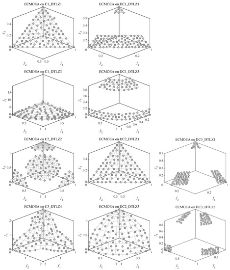
Figure A2.
Feasible and non-dominated solution sets obtained by ECMOEA on DTLZ instances with the median IGD value among 30 runs.
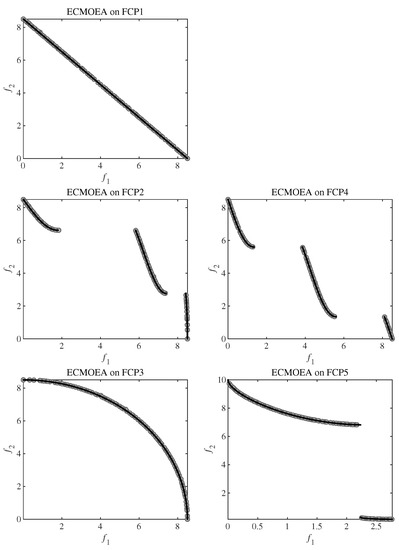
Figure A3.
Feasible and non-dominated solution sets obtained by ECMOEA on FCP instances with the median IGD value among 30 runs.
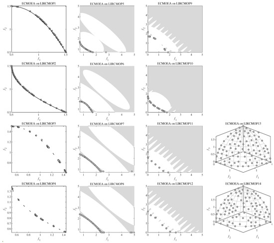
Figure A4.
Feasible and non-dominated solution sets obtained by ECMOEA on LIR-CMOP instances with the median IGD value among 30 runs.
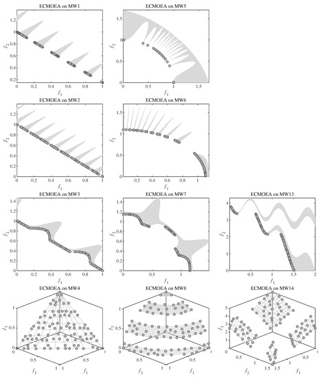
Figure A5.
Feasible and non-dominated solution sets obtained by ECMOEA on MW instances with the median IGD value among 30 runs.
Table A11.
Statistical results of HV obtained by ECMOEA and CMOEAs in comparison on DAS-CMOP benchmark problems. Best result in each row is highlighted.
Table A11.
Statistical results of HV obtained by ECMOEA and CMOEAs in comparison on DAS-CMOP benchmark problems. Best result in each row is highlighted.
| Problem | CMOEA_MS | CTAEA | DCNSGAIII | MOEADDAE | NSGAIIToR | TiGE2 | ToP | ECMOEA |
|---|---|---|---|---|---|---|---|---|
| DASCMOP1 | 7.4593 × (1.21 × ) − | 1.6794 × (1.88 × ) − | 1.1349 × (1.54 × ) − | 2.2463 × (2.70 × ) − | 6.6340 × (2.09 × ) − | 2.6584 × (3.69 × ) − | 7.7065 × (1.15 × ) − | 2.1202 × (4.62 × ) |
| DASCMOP2 | 2.5503 × (4.28 × ) − | 3.0341 × (8.08 × ) − | 2.4932 × (4.39 × ) − | 2.8031 × (1.98 × ) − | 1.2786 × (9.84 × ) − | 2.6909 × (1.18 × ) − | 6.6653 × (8.09 × ) − | 3.5504 × (7.11 × ) |
| DASCMOP3 | 2.0854 × (1.98 × ) − | 2.4766 × (1.38 × ) − | 2.2136 × (1.43 × ) − | 2.2492 × (3.69 × ) − | 1.0781 × (1.15 × ) − | 2.1562 × (1.61 × ) − | 1.7942 × (1.28 × ) − | 3.1191 × (4.13 × ) |
| DASCMOP4 | 1.8476 × (3.65 × ) ≈ | 1.9554 × (4.94 × ) ≈ | 1.9591 × (3.33 × ) ≈ | 2.0212 × (4.67 × ) + | NaN (NaN) | 1.9157 × (7.48 × ) ≈ | NaN (NaN) | 1.7485 × (4.48 × ) |
| DASCMOP5 | 3.0368 × (9.72 × ) − | 3.4768 × (7.89 × ) + | 3.4870 × (1.12 × ) + | 3.4936 × (2.44 × ) ≈ | NaN (NaN) | 3.3960 × (2.54 × ) + | NaN (NaN) | 3.3874 × (4.35 × ) |
| DASCMOP6 | 1.3157 × (1.02 × ) − | 3.0726 × (1.36 × ) ≈ | 2.9766 × (4.05 × ) ≈ | 2.9354 × (2.21 × ) ≈ | NaN (NaN) | 2.9130 × (5.21 × ) ≈ | NaN (NaN) | 2.4548 × (9.70 × ) |
| DASCMOP7 | 2.8840 × (2.27 × ) + | 2.8722 × (1.73 × ) ≈ | 2.8078 × (1.50 × ) + | 2.8473 × (1.42 × ) + | NaN (NaN) | 2.6270 × (8.54 × ) − | NaN (NaN) | 2.7886 × (1.84 × ) |
| DASCMOP8 | 2.0721 × (3.04 × ) + | 2.0349 × (1.33 × ) + | 1.9725 × (2.07 × ) − | 2.0293 × (2.96 × ) + | NaN (NaN) | 1.8381 × (7.73 × ) − | NaN (NaN) | 1.9989 × (1.74 × ) |
| DASCMOP9 | 1.2340 × (1.26 × ) − | 1.4192 × (1.00 × ) − | 1.1904 × (1.45 × ) − | 1.1041 × (3.76 × ) − | 5.7373 × (8.76 × ) − | 1.3743 × (1.06 × ) − | 6.2156 × (2.01 × ) − | 2.0613 × (2.33 × ) |
| × | 2/6/1 | 2/4/3 | 2/5/2 | 3/4/2 | 0/4/0 | 1/6/2 | 0/4/0 |
Table A12.
Statistical results of IGD obtained by ECMOEA and CMOEAs in comparison on DAS-CMOP benchmark problems. Best result in each row is highlighted.
Table A12.
Statistical results of IGD obtained by ECMOEA and CMOEAs in comparison on DAS-CMOP benchmark problems. Best result in each row is highlighted.
| Problem | CMOEA_MS | CTAEA | DCNSGAIII | MOEADDAE | NSGAIIToR | TiGE2 | ToP | ECMOEA |
|---|---|---|---|---|---|---|---|---|
| DASCMOP1 | 7.4102 × (3.70 × ) − | 1.8777 × (1.25 × ) − | 7.2850 × (2.86 × ) − | 7.1755 × (4.09 × ) − | 8.1427 × (3.00 × ) − | 6.3691 × (1.27 × ) − | 7.5260 × (8.61 × ) − | 3.9235 × (5.39 × ) |
| DASCMOP2 | 2.6022 × (3.66 × ) − | 9.7215 × (2.74 × ) − | 2.8495 × (3.71 × ) − | 2.1359 × (4.29 × ) − | 5.3228 × (2.33 × ) − | 2.0882 × (6.58 × ) − | 6.6475 × (2.15 × ) − | 4.7686 × (1.02 × ) |
| DASCMOP3 | 3.5417 × (3.09 × ) − | 1.6825 × (5.36 × ) − | 2.7035 × (3.10 × ) − | 2.8789 × (1.11 × ) − | 7.9033 × (6.08 × ) − | 3.2257 × (5.22 × ) − | 7.5129 × (5.45 × ) − | 1.9721 × (1.18 × ) |
| DASCMOP4 | 4.6356 × (9.92 × ) ≈ | 1.2134 × (2.38 × ) ≈ | 5.6580 × (1.32 × ) ≈ | 3.1917 × (4.35 × ) ≈ | NaN (NaN) | 2.8533 × (1.13 × ) ≈ | NaN (NaN) | 7.8203 × (1.17 × ) |
| DASCMOP5 | 8.1958 × (1.62 × ) − | 7.9797 × (8.72 × ) + | 6.9278 × (3.15 × ) + | 5.2862 × (2.27 × ) + | NaN (NaN) | 2.7598 × (4.94 × ) − | NaN (NaN) | 2.2552 × (6.96 × ) |
| DASCMOP6 | 3.6123 × (1.87 × ) − | 2.7557 × (3.75 × ) ≈ | 5.2111 × (8.32 × ) ≈ | 6.3304 × (5.63 × ) ≈ | NaN (NaN) | 7.2012 × (1.23 × ) ≈ | NaN (NaN) | 1.5724 × (2.12 × ) |
| DASCMOP7 | 3.2090 × (8.48 × ) ≈ | 3.8548 × (3.74 × ) + | 4.1958 × (2.55 × ) + | 3.8577 × (3.88 × ) + | NaN (NaN) | 1.1142 × (2.61 × ) − | NaN (NaN) | 5.0821 × (3.96 × ) |
| DASCMOP8 | 4.1598 × (8.78 × ) + | 5.5200 × (4.60 × ) + | 8.5478 × (1.23 × ) − | 5.3687 × (7.81 × ) + | NaN (NaN) | 1.4476 × (3.02 × ) − | NaN (NaN) | 5.5965 × (3.30 × ) |
| DASCMOP9 | 4.0198 × (7.69 × ) − | 2.5623 × (5.11 × ) − | 4.0811 × (9.38 × ) − | 4.5442 × (1.99 × ) − | 6.9550 × (9.10 × ) − | 2.7409 × (4.91 × ) − | 6.9131 × (1.59 × ) − | 4.3039 × (8.96 × ) |
| × | 1/6/2 | 3/4/2 | 2/5/2 | 3/4/2 | 0/4/0 | 0/7/2 | 0/4/0 |
Table A13.
Statistical results of HV obtained by ECMOEA and CMOEAs in comparison on DTLZ benchmark problems. Best result in each row is highlighted.
Table A13.
Statistical results of HV obtained by ECMOEA and CMOEAs in comparison on DTLZ benchmark problems. Best result in each row is highlighted.
| Problem | CMOEA_MS | CTAEA | DCNSGAIII | MOEADDAE | NSGAIIToR | TiGE2 | ToP | ECMOEA |
|---|---|---|---|---|---|---|---|---|
| C1-DTLZ1 | 8.3539 × (3.15 × ) ≈ | 8.3645 × (1.66 × ) ≈ | 8.3891 × (3.76 × ) + | 8.3977 × (2.45 × ) + | NaN (NaN) | 2.3202 × (1.60 × ) − | NaN (NaN) | 8.3117 × (9.67 × ) |
| C1-DTLZ3 | 5.5686 × (1.66 × ) ≈ | 4.4184 × (1.75 × ) − | 2.2320 × (2.74 × ) − | 5.5639 × (1.64 × ) ≈ | 0.0000 × (0.00 × ) − | 0.0000 × (0.00 × ) − | 2.9100 × (2.08 × ) − | 5.5559 × (6.92 × ) |
| C2-DTLZ2 | 5.1551 × (1.36 × ) + | 5.0680 × (2.18 × ) − | 5.0676 × (1.55 × ) − | 5.1515 × (1.89 × ) + | 3.1487 × (2.50 × ) − | 4.3699 × (3.49 × ) − | 4.5579 × (3.14 × ) − | 5.1346 × (1.64 × ) |
| C3-DTLZ4 | 4.7153 × (6.89 × ) − | 7.8531 × (9.95 × ) − | 7.5568 × (8.98 × ) ≈ | 4.6011 × (1.81 × ) − | 4.7327 × (1.97 × ) − | 7.6502 × (3.30 × ) − | 7.5181 × (4.15 × ) − | 7.9059 × (8.34 × ) |
| DC1-DTLZ1 | 6.1513 × (2.12 × ) − | 6.2714 × (1.01 × ) − | 6.2505 × (2.15 × ) − | 6.3229 × (5.59 × ) + | 0.0000 × (0.00 × ) − | 5.2909 × (6.00 × ) − | 5.6523 × (2.49 × ) − | 6.3048 × (1.77 × ) |
| DC1-DTLZ3 | 4.3719 × (5.51 × ) ≈ | 4.6142 × (2.28 × ) − | 4.6752 × (1.63 × ) + | 4.7401 × (9.33 × ) + | 0.0000 × (0.00 × ) − | 0.0000 × (0.00 × ) − | 7.9346 × (1.15 × ) − | 4.6722 × (2.48 × ) |
| DC2-DTLZ1 | 8.2582 × (6.47 × ) + | 8.3795 × (5.24 × ) + | 6.5774 × (2.00 × ) ≈ | 8.4078 × (3.25 × ) + | NaN (NaN) | 2.2905 × (7.11 × ) − | NaN (NaN) | 8.1760 × (7.45 × ) |
| DC2-DTLZ3 | 1.7637 × (2.54 × ) ≈ | 2.4441 × (2.65 × ) − | 7.3796 × (2.09 × ) − | 1.6913 × (2.45 × ) ≈ | NaN (NaN) | 0.0000 × (0.00 × ) ≈ | NaN (NaN) | 4.4170 × (1.82 × ) |
| DC3-DTLZ1 | 4.1023 × (4.92 × ) − | 5.2363 × (3.01 × ) − | 5.2854 × (1.72 × ) − | 4.4886 × (1.75 × ) ≈ | 0.0000 × (0.00 × ) − | 2.6655 × (1.46 × ) − | 5.3504 × (2.05 × ) − | 5.3397 × (2.92 × ) |
| DC3-DTLZ3 | 2.6430 × (1.63 × ) + | 3.5048 × (1.94 × ) + | 1.2019 × (6.58 × ) − | 1.3624 × (1.63 × ) ≈ | 0.0000 × (0.00 × ) − | 0.0000 × (0.00 × ) − | 0.0000 × (0.00 × ) − | 1.8319 × (1.59 × ) |
| × | 3/3/4 | 2/7/1 | 2/6/2 | 5/1/4 | 0/7/0 | 0/9/1 | 0/7/0 |
Table A14.
Statistical results of IGD obtained by ECMOEA and CMOEAs in comparison on DTLZ benchmark problems. Best result in each row is highlighted.
Table A14.
Statistical results of IGD obtained by ECMOEA and CMOEAs in comparison on DTLZ benchmark problems. Best result in each row is highlighted.
| Problem | CMOEA_MS | CTAEA | DCNSGAIII | MOEADDAE | NSGAIIToR | TiGE2 | ToP | ECMOEA |
|---|---|---|---|---|---|---|---|---|
| C1-DTLZ1 | 2.1505 × (2.44 × ) ≈ | 2.3216 × (2.43 × ) − | 2.0411 × (1.23 × ) + | 2.1039 × (1.11 × ) + | NaN (NaN) | 3.3618 × (9.78 × ) − | NaN (NaN) | 2.2863 × (2.55 × ) |
| C1-DTLZ3 | 5.5983 × (5.32 × ) + | 2.6155 × (5.64 × ) − | 4.4120 × (3.95 × ) − | 6.3937 × (4.88 × ) − | 1.5109 × (3.28 × ) − | 6.4159 × (3.02 × ) − | 1.1084 × (2.40 × ) − | 5.7235 × (3.87 × ) |
| C2-DTLZ2 | 4.4480 × (5.37 × ) + | 5.6530 × (1.16 × ) − | 4.8055 × (5.12 × ) − | 4.4140 × (5.20 × ) + | 2.2981 × (4.16 × ) − | 1.1979 × (3.76 × ) − | 6.7908 × (2.07 × ) − | 4.4994 × (4.98 × ) |
| C3-DTLZ4 | 6.8251 × (6.92 × ) − | 1.1156 × (1.85 × ) − | 1.9617 × (2.58 × ) − | 7.3140 × (3.70 × ) − | 7.8185 × (4.97 × ) − | 1.9485 × (1.21 × ) − | 1.4775 × (4.83 × ) − | 1.0285 × (1.51 × ) |
| DC1-DTLZ1 | 1.6840 × (5.92 × ) − | 1.5336 × (2.71 × ) − | 1.3772 × (1.88 × ) − | 1.2079 × (7.48 × ) + | 1.3100 × (5.80 × ) − | 6.0613 × (2.79 × ) − | 2.6383 × (6.41 × ) − | 1.2178 × (1.84 × ) |
| DC1-DTLZ3 | 1.3150 × (1.49 × ) ≈ | 4.3320 × (1.29 × ) + | 4.6115 × (8.78 × ) + | 3.6595 × (1.13 × ) + | 1.3494 × (2.79 × ) − | 2.2495 × (6.97 × ) − | 1.3916 × (1.48 × ) − | 4.6968 × (6.10 × ) |
| DC2-DTLZ1 | 2.6494 × (2.59 × ) + | 2.3194 × (1.98 × ) + | 9.2959 × (7.91 × ) ≈ | 2.1173 × (1.58 × ) + | NaN (NaN) | 3.4202 × (5.38 × ) − | NaN (NaN) | 2.8151 × (2.73 × ) |
| DC2-DTLZ3 | 4.1012 × (2.36 × ) ≈ | 3.4190 × (2.51 × ) − | 5.8320 × (7.08 × ) − | 4.1457 × (2.31 × ) − | NaN (NaN) | 7.1406 × (0.00 × ) ≈ | NaN (NaN) | 1.4449 × (1.73 × ) |
| DC3-DTLZ1 | 3.4208 × (1.05 × ) − | 9.4040 × (2.48 × ) − | 1.0045 × (3.07 × ) − | 3.9794 × (6.57 × ) − | 7.7910 × (3.62 × ) − | 1.6313 × (1.09 × ) − | 3.7754 × (4.04 × ) − | 7.3281 × (1.26 × ) |
| DC3-DTLZ3 | 2.3006 × (3.88 × ) + | 3.2940 × (1.63 × ) + | 6.0756 × (2.30 × ) − | 6.0916 × (6.04 × ) ≈ | 5.4843 × (1.24 × ) − | 4.2603 × (1.26 × ) − | 8.7643 × (3.29 × ) − | 2.6746 × (2.54 × ) |
| × | 4/3/3 | 3/7/0 | 2/7/1 | 5/4/1 | 0/7/0 | 0/9/1 | 0/7/0 |
Table A15.
Statistical results of HV obtained by ECMOEA and CMOEAs in comparison on FCP benchmark problems. Best result in each row is highlighted.
Table A15.
Statistical results of HV obtained by ECMOEA and CMOEAs in comparison on FCP benchmark problems. Best result in each row is highlighted.
| Problem | CMOEA_MS | CTAEA | DCNSGAIII | MOEADDAE | NSGAIIToR | TiGE2 | ToP | ECMOEA |
|---|---|---|---|---|---|---|---|---|
| FCP1 | NaN (NaN) | NaN (NaN) | NaN (NaN) | NaN (NaN) | NaN (NaN) | NaN (NaN) | NaN (NaN) | 5.8083 × (1.37 × ) |
| FCP2 | NaN (NaN) | NaN (NaN) | NaN (NaN) | NaN (NaN) | NaN (NaN) | NaN (NaN) | NaN (NaN) | 4.3120 × (1.92 × ) |
| FCP3 | NaN (NaN) | NaN (NaN) | NaN (NaN) | NaN (NaN) | NaN (NaN) | NaN (NaN) | NaN (NaN) | 3.4653 × (1.48 × ) |
| FCP4 | NaN (NaN) | NaN (NaN) | NaN (NaN) | NaN (NaN) | NaN (NaN) | NaN (NaN) | NaN (NaN) | 6.3374 × (4.57 × ) |
| FCP5 | 1.4401 × (1.05 × ) − | 2.2982 × (2.37 × ) − | NaN (NaN) | 2.4344 × (3.14 × ) − | 3.8618 × (8.25 × ) − | 2.5879 × (1.90 × ) − | 5.3780 × (5.24 × ) − | 4.2380 × (9.07 × ) |
| × | 0/1/0 | 0/1/0 | 0/0/0 | 0/1/0 | 0/1/0 | 0/1/0 | 0/1/0 |
Table A16.
Statistical results of IGD obtained by ECMOEA and CMOEAs in comparison on FCP benchmark problems. Best result in each row is highlighted.
Table A16.
Statistical results of IGD obtained by ECMOEA and CMOEAs in comparison on FCP benchmark problems. Best result in each row is highlighted.
| Problem | CMOEA_MS | CTAEA | DCNSGAIII | MOEADDAE | NSGAIIToR | TiGE2 | ToP | ECMOEA |
|---|---|---|---|---|---|---|---|---|
| FCP1 | NaN (NaN) | NaN (NaN) | NaN (NaN) | NaN (NaN) | NaN (NaN) | NaN (NaN) | NaN (NaN) | 3.9006 × (7.10 × ) |
| FCP2 | NaN (NaN) | NaN (NaN) | NaN (NaN) | NaN (NaN) | NaN (NaN) | NaN (NaN) | NaN (NaN) | 3.9383 × (1.03 × ) |
| FCP3 | NaN (NaN) | NaN (NaN) | NaN (NaN) | NaN (NaN) | NaN (NaN) | NaN (NaN) | NaN (NaN) | 4.2828 × (1.24 × ) |
| FCP4 | NaN (NaN) | NaN (NaN) | NaN (NaN) | NaN (NaN) | NaN (NaN) | NaN (NaN) | NaN (NaN) | 3.0694 × (1.50 × ) |
| FCP5 | 4.4497 × (2.03 × ) − | 4.7115 × (2.44 × ) − | NaN (NaN) | 4.7154 × (4.20 × ) − | 4.4003 × (5.41 × ) − | 4.7030 × (9.14 × ) − | 4.2664 × (6.63 × ) − | 1.1119 × (2.00 × ) |
| × | 0/1/0 | 0/1/0 | 0/0/0 | 0/1/0 | 0/1/0 | 0/1/0 | 0/1/0 |
Table A17.
Statistical results of HV obtained by ECMOEA and CMOEAs in comparison on LIR-CMOP benchmark problems. Best result in each row is highlighted.
Table A17.
Statistical results of HV obtained by ECMOEA and CMOEAs in comparison on LIR-CMOP benchmark problems. Best result in each row is highlighted.
| Problem | CMOEA_MS | CTAEA | DCNSGAIII | MOEADDAE | NSGAIIToR | TiGE2 | ToP | ECMOEA |
|---|---|---|---|---|---|---|---|---|
| LIRCMOP1 | 1.0115 × (1.19 × ) − | 1.1848 × (2.50 × ) − | 1.4984 × (9.90 × ) − | 1.5432 × (1.73 × ) − | 9.5614 × (5.70 × ) − | 1.3806 × (6.46 × ) − | 1.0697 × (9.48 × ) − | 2.2184 × (1.41 × ) |
| LIRCMOP2 | 2.1842 × (1.55 × ) − | 2.6877 × (3.56 × ) − | 2.7303 × (9.13 × ) − | 2.8306 × (1.56 × ) − | 2.0501 × (8.62 × ) − | 2.6404 × (8.71 × ) − | 2.1595 × (1.13 × ) − | 3.5079 × (7.94 × ) |
| LIRCMOP3 | 9.5727 × (1.27 × ) − | 9.9812 × (1.86 × ) − | 1.3522 × (1.16 × ) − | 1.4090 × (1.76 × ) − | 8.8113 × (4.73 × ) − | 1.2159 × (1.02 × ) − | 9.1838 × (5.94 × ) − | 1.8854 × (1.36 × ) |
| LIRCMOP4 | 1.9142 × (1.59 × ) − | 1.8915 × (2.48 × ) − | 2.3185 × (1.32 × ) − | 2.3742 × (1.66 × ) − | 1.7744 × (8.34 × ) − | 2.2264 × (1.37 × ) − | 1.8521 × (8.38 × ) − | 2.8486 × (2.73 × ) |
| LIRCMOP5 | 1.3969 × (4.27 × ) − | 2.2548 × (5.29 × ) − | 1.0042 × (7.35 × ) − | 1.4195 × (1.62 × ) − | 0.0000 × (0.00 × ) − | 1.4329 × (4.39 × ) − | 3.2396 × (1.77 × ) − | 2.8993 × (1.09 × ) |
| LIRCMOP6 | 8.7194 × (3.59 × ) − | 2.7802 × (1.52 × ) − | 6.0182 × (5.03 × ) − | 1.0163 × (8.32 × ) − | 0.0000 × (0.00 × ) − | 1.9501 × (3.35 × ) − | 1.8838 × (1.03 × ) − | 1.9391 × (6.44 × ) |
| LIRCMOP7 | 2.3623 × (4.56 × ) − | 2.3310 × (4.53 × ) − | 2.4779 × (5.93 × ) − | 2.3852 × (7.38 × ) − | 0.0000 × (0.00 × ) − | 1.9448 × (3.27 × ) − | 2.9611 × (7.80 × ) − | 2.7155 × (1.91 × ) |
| LIRCMOP8 | 2.2770 × (7.63 × ) − | 1.2629 × (1.01 × ) − | 2.2658 × (4.24 × ) − | 2.2320 × (5.27 × ) − | 0.0000 × (0.00 × ) − | 1.7051 × (5.00 × ) − | 3.6019 × (7.53 × ) − | 2.8425 × (1.70 × ) |
| LIRCMOP9 | 2.9951 × (7.05 × ) − | 3.5948 × (5.49 × ) − | 2.6570 × (7.27 × ) − | 4.8049 × (6.35 × ) + | 3.7327 × (1.14 × ) − | 2.2646 × (9.34 × ) − | 3.0712 × (7.43 × ) − | 4.7741 × (2.89 × ) |
| LIRCMOP10 | 4.6143 × (8.76 × ) − | 5.1822 × (2.12 × ) − | 3.7586 × (1.93 × ) − | 6.3167 × (1.23 × ) ≈ | 7.3311 × (2.62 × ) − | 1.2391 × (4.61 × ) − | 4.6129 × (8.92 × ) − | 6.7585 × (3.22 × ) |
| LIRCMOP11 | 4.9685 × (1.09 × ) − | 5.9640 × (2.79 × ) − | 5.4404 × (9.82 × ) − | 5.9932 × (1.33 × ) − | 6.4728 × (3.41 × ) − | 1.9026 × (1.06 × ) − | 4.0354 × (8.82 × ) − | 6.7327 × (2.91 × ) |
| LIRCMOP12 | 4.5963 × (4.49 × ) − | 4.9804 × (4.56 × ) − | 4.7283 × (4.22 × ) − | 5.8668 × (2.83 × ) ≈ | 7.8454 × (1.76 × ) − | 3.5124 × (5.79 × ) − | 4.6303 × (4.34 × ) − | 5.8864 × (2.42 × ) |
| LIRCMOP13 | 5.5352 × (1.32 × ) + | 5.4607 × (1.34 × ) − | 4.1686 × (7.50 × ) − | 5.5500 × (1.30 × ) + | 4.3729 × (2.40 × ) − | 1.7644 × (7.74 × ) − | 2.0082 × (1.08 × ) − | 5.5170 × (1.14 × ) |
| LIRCMOP14 | 5.5298 × (1.23 × ) + | 5.4605 × (7.72 × ) − | 9.4256 × (6.07 × ) − | 5.5319 × (1.09 × ) + | 3.3677 × (1.70 × ) − | 3.8556 × (8.91 × ) − | 1.1349 × (3.03 × ) − | 5.5091 × (1.62 × ) |
| × | 2/12/0 | 0/14/0 | 0/14/0 | 3/9/2 | 0/14/0 | 0/14/0 | 0/14/0 |
Table A18.
Statistical results of IGD obtained by ECMOEA and CMOEAs in comparison on LIR-CMOP benchmark problems. Best result in each row is highlighted.
Table A18.
Statistical results of IGD obtained by ECMOEA and CMOEAs in comparison on LIR-CMOP benchmark problems. Best result in each row is highlighted.
| Problem | CMOEA_MS | CTAEA | DCNSGAIII | MOEADDAE | NSGAIIToR | TiGE2 | ToP | ECMOEA |
|---|---|---|---|---|---|---|---|---|
| LIRCMOP1 | 3.4677 × (4.82 × ) − | 3.0267 × (9.72 × ) − | 1.8277 × (2.38 × ) − | 1.7492 × (3.87 × ) − | 3.6403 × (9.72 × ) − | 2.1918 × (1.78 × ) − | 3.2074 × (2.00 × ) − | 4.0024 × (3.57 × ) |
| LIRCMOP2 | 2.8670 × (3.19 × ) − | 2.1030 × (8.58 × ) − | 1.8254 × (2.00 × ) − | 1.6174 × (4.41 × ) − | 3.2103 × (7.43 × ) − | 1.9561 × (1.77 × ) − | 2.8707 × (1.13 × ) − | 2.5367 × (1.84 × ) |
| LIRCMOP3 | 3.2784 × (4.29 × ) − | 3.2563 × (8.99 × ) − | 1.8986 × (3.58 × ) − | 1.8257 × (4.71 × ) − | 3.5146 × (7.84 × ) − | 2.3604 × (2.85 × ) − | 3.4335 × (1.38 × ) − | 4.8873 × (3.63 × ) |
| LIRCMOP4 | 3.0059 × (3.46 × ) − | 3.2288 × (7.81 × ) − | 2.1136 × (2.83 × ) − | 1.9991 × (3.76 × ) − | 3.2496 × (6.76 × ) − | 2.1999 × (2.44 × ) − | 3.0962 × (1.05 × ) − | 7.1909 × (5.97 × ) |
| LIRCMOP5 | 3.7935 × (2.29 × ) − | 1.0849 × (3.32 × ) − | 6.1546 × (4.40 × ) − | 3.3377 × (3.33 × ) − | 2.6644 × (5.86 × ) − | 1.1355 × (2.67 × ) − | 1.1825 × (9.90 × ) − | 9.0963 × (1.35 × ) |
| LIRCMOP6 | 5.0145 × (3.50 × ) − | 1.3149 × (1.72 × ) − | 7.5519 × (4.95 × ) − | 3.6595 × (6.89 × ) − | 2.8305 × (2.96 × ) − | 1.1605 × (3.43 × ) − | 1.3224 × (1.35 × ) − | 1.5276 × (2.00 × ) |
| LIRCMOP7 | 1.8769 × (2.84 × ) − | 1.9967 × (2.83 × ) − | 1.1912 × (2.03 × ) − | 1.4512 × (2.65 × ) − | 2.9434 × (6.40 × ) − | 3.3566 × (1.45 × ) − | 1.4870 × (5.13 × ) − | 5.9428 × (4.55 × ) |
| LIRCMOP8 | 2.1669 × (4.42 × ) − | 8.5644 × (6.60 × ) − | 2.1996 × (3.13 × ) − | 2.2209 × (3.22 × ) − | 3.0160 × (6.92 × ) − | 5.2013 × (3.45 × ) − | 1.4431 × (5.04 × ) − | 3.2441 × (4.54 × ) |
| LIRCMOP9 | 6.3197 × (1.12 × ) − | 4.8471 × (9.91 × ) − | 7.8136 × (1.48 × ) − | 2.5027 × (1.51 × ) ≈ | 1.2696 × (5.72 × ) − | 7.7593 × (1.94 × ) − | 5.6230 × (1.20 × ) − | 2.2752 × (8.98 × ) |
| LIRCMOP10 | 4.3915 × (9.85 × ) − | 3.4745 × (3.97 × ) − | 4.5050 × (2.81 × ) − | 1.1462 × (1.90 × ) ≈ | 1.0588 × (6.48 × ) − | 9.6528 × (1.86 × ) − | 4.3900 × (8.54 × ) − | 7.4373 × (7.04 × ) |
| LIRCMOP11 | 3.2899 × (1.41 × ) − | 2.3137 × (5.53 × ) − | 2.7798 × (1.59 × ) − | 2.3136 × (3.29 × ) − | 1.3025 × (2.02 × ) − | 8.4857 × (2.98 × ) − | 4.4492 × (1.23 × ) − | 3.8158 × (4.76 × ) |
| LIRCMOP12 | 3.4010 × (9.10 × ) − | 2.4646 × (1.18 × ) − | 4.0424 × (1.64 × ) − | 9.9434 × (1.24 × ) ≈ | 1.3856 × (7.24 × ) − | 5.3323 × (1.34 × ) − | 3.1937 × (8.51 × ) − | 7.4168 × (5.49 × ) |
| LIRCMOP13 | 9.7025 × (8.88 × ) + | 1.0935 × (2.26 × ) − | 1.3068 × (8.78 × ) − | 9.7361 × (8.88 × ) + | 1.5044 × (3.85 × ) − | 1.3954 × (2.04 × ) − | 1.3376 × (6.20 × ) − | 9.8540 × (1.15 × ) |
| LIRCMOP14 | 9.9381 × (9.46 × ) + | 1.1116 × (1.19 × ) − | 1.2631 × (8.75 × ) − | 9.9770 × (6.42 × ) + | 1.4943 × (4.78 × ) − | 1.2359 × (3.01 × ) − | 1.2611 × (1.25 × ) − | 1.0417 × (3.49 × ) |
| × | 2/12/0 | 0/14/0 | 0/14/0 | 2/9/3 | 0/14/0 | 0/14/0 | 0/14/0 |
Table A19.
Statistical results of HV obtained by ECMOEA and CMOEAs in comparison on MW benchmark problems. Best result in each row is highlighted.
Table A19.
Statistical results of HV obtained by ECMOEA and CMOEAs in comparison on MW benchmark problems. Best result in each row is highlighted.
| Problem | CMOEA_MS | CTAEA | DCNSGAIII | MOEADDAE | NSGAIIToR | TiGE2 | ToP | ECMOEA |
|---|---|---|---|---|---|---|---|---|
| MW1 | 4.8676 × (5.96 × ) ≈ | 4.8748 × (3.16 × ) − | 4.8869 × (2.21 × ) − | 4.8443 × (2.36 × ) ≈ | 1.7502 × (3.91 × ) − | 4.3587 × (4.58 × ) − | NaN (NaN) | 4.8916 × (1.48 × ) |
| MW2 | 5.4292 × (1.89 × ) − | 5.5433 × (1.36 × ) − | 5.5963 × (1.33 × ) − | 5.1308 × (3.59 × ) − | 4.1775 × (7.39 × ) − | 5.2809 × (1.34 × ) − | 3.7255 × (1.50 × ) − | 5.7126 × (1.07 × ) |
| MW3 | 5.4345 × (6.46 × ) − | 5.4417 × (6.39 × ) ≈ | 5.4419 × (5.93 × ) ≈ | 5.4329 × (5.46 × ) − | 2.6028 × (1.19 × ) − | 5.2152 × (2.26 × ) − | 2.1977 × (1.88 × ) − | 5.4418 × (2.99 × ) |
| MW4 | 8.3732 × (8.52 × ) + | 8.3815 × (2.25 × ) + | 8.4122 × (3.24 × ) + | 8.3998 × (4.49 × ) + | 2.9498 × (8.83 × ) − | 7.5894 × (4.59 × ) − | NaN (NaN) | 8.2426 × (1.76 × ) |
| MW5 | 2.8635 × (3.85 × ) − | 3.1594 × (1.87 × ) ≈ | 3.0727 × (2.57 × ) − | 3.2158 × (4.72 × ) + | 3.4284 × (1.14 × ) − | 2.8655 × (1.22 × ) − | 3.7421 × (2.53 × ) − | 3.1721 × (4.36 × ) |
| MW6 | 2.9857 × (1.41 × ) − | 3.1097 × (9.79 × ) ≈ | 3.0777 × (2.03 × ) ≈ | 2.6193 × (4.41 × ) − | 1.3821 × (4.00 × ) − | 2.0971 × (8.06 × ) − | 5.4799 × (6.31 × ) − | 3.1025 × (1.47 × ) |
| MW7 | 4.0729 × (4.03 × ) − | 4.0863 × (8.45 × ) − | 4.1127 × (4.34 × ) − | 4.1184 × (3.67 × ) ≈ | 2.6471 × (6.16 × ) − | 3.8964 × (4.43 × ) − | 3.4344 × (7.72 × ) − | 4.1184 × (5.86 × ) |
| MW8 | 5.2026 × (1.47 × ) ≈ | 5.2489 × (1.04 × ) ≈ | 5.3028 × (1.08 × ) ≈ | 4.9523 × (5.01 × ) − | 3.0869 × (6.99 × ) − | 3.5317 × (1.45 × ) − | 8.6399 × (1.01 × ) − | 5.2682 × (1.40 × ) |
| MW9 | 2.3871 × (1.75 × ) − | 3.9125 × (2.03 × ) ≈ | 3.8276 × (5.89 × ) + | 3.9811 × (3.71 × ) + | 1.0307 × (5.80 × ) − | 2.9342 × (1.36 × ) − | 0.0000 × (0.00 × ) ≈ | 3.8030 × (5.76 × ) |
| MW10 | 4.0682 × (2.53 × ) − | 4.3743 × (1.56 × ) + | 4.2341 × (1.83 × ) ≈ | 3.6348 × (7.40 × ) − | 2.4674 × (8.80 × ) − | 3.7718 × (5.21 × ) − | NaN (NaN) | 4.1951 × (1.84 × ) |
| MW11 | 4.2975 × (5.16 × ) ≈ | 4.4139 × (1.35 × ) − | 4.4215 × (3.73 × ) − | 4.4494 × (5.57 × ) − | 2.5121 × (5.09 × ) − | 4.3473 × (2.57 × ) − | 2.7045 × (2.93 × ) − | 4.4708 × (2.65 × ) |
| MW12 | 6.0336 × (5.03 × ) − | 6.0006 × (7.21 × ) − | 5.8159 × (1.07 × ) − | 4.8591 × (2.39 × ) − | 1.3563 × (3.42 × ) − | 4.9320 × (1.98 × ) − | 2.7375 × (6.71 × ) − | 6.0390 × (3.86 × ) |
| MW13 | 4.3660 × (1.71 × ) − | 4.5761 × (1.49 × ) ≈ | 4.4369 × (1.22 × ) − | 4.1742 × (3.06 × ) − | 2.0166 × (4.79 × ) − | 3.1646 × (3.37 × ) − | 1.7326 × (1.11 × ) − | 4.5707 × (1.33 × ) |
| MW14 | 4.6322 × (5.06 × ) − | 4.6632 × (2.76 × ) − | 4.6276 × (8.80 × ) − | 4.7451 × (1.63 × ) + | 3.9445 × (7.44 × ) − | 4.4657 × (4.74 × ) − | 3.2108 × (1.68 × ) − | 4.7087 × (2.64 × ) |
| × | 1/10/3 | 2/6/6 | 2/8/4 | 4/8/2 | 0/14/0 | 0/14/0 | 0/10/1 |
Table A20.
Statistical results of IGD obtained by ECMOEA and CMOEAs in comparison on MW benchmark problems. Best result in each row is highlighted.
Table A20.
Statistical results of IGD obtained by ECMOEA and CMOEAs in comparison on MW benchmark problems. Best result in each row is highlighted.
| Problem | CMOEA_MS | CTAEA | DCNSGAIII | MOEADDAE | NSGAIIToR | TiGE2 | ToP | ECMOEA |
|---|---|---|---|---|---|---|---|---|
| MW1 | 3.4592 × (3.10 × ) − | 2.7882 × (1.62 × ) − | 2.5748 × (9.80 × ) − | 7.3274 × (2.50 × ) − | 6.5822 × (1.25 × ) − | 5.2793 × (5.54 × ) − | NaN (NaN) | 1.9580 × (5.74 × ) |
| MW2 | 2.7738 × (1.24 × ) − | 2.0019 × (8.16 × ) − | 1.6904 × (7.66 × ) − | 4.8670 × (2.65 × ) − | 1.4076 × (9.48 × ) − | 3.8754 × (1.23 × ) − | 1.8214 × (1.80 × ) − | 1.0474 × (5.85 × ) |
| MW3 | 5.9683 × (3.37 × ) − | 5.5917 × (4.27 × ) ≈ | 6.9186 × (8.62 × ) − | 5.8576 × (2.87 × ) − | 3.7038 × (2.40 × ) − | 3.5421 × (3.43 × ) − | 4.9445 × (3.59 × ) − | 5.6406 × (3.73 × ) |
| MW4 | 4.3942 × (6.27 × ) + | 4.6598 × (3.30 × ) + | 4.1681 × (4.31 × ) + | 4.2948 × (4.38 × ) + | 4.5506 × (1.25 × ) − | 1.1416 × (5.25 × ) − | NaN (NaN) | 5.1730 × (8.68 × ) |
| MW5 | 7.3763 × (8.91 × ) − | 1.4026 × (2.86 × ) − | 3.9050 × (9.23 × ) − | 4.8949 × (6.58 × ) + | 7.7006 × (1.43 × ) − | 5.9433 × (1.75 × ) − | 3.7858 × (2.91 × ) − | 9.9150 × (5.40 × ) |
| MW6 | 2.3006 × (1.04 × ) − | 1.2619 × (6.48 × ) ≈ | 1.6373 × (1.52 × ) ≈ | 7.5654 × (1.16 × ) − | 5.1466 × (1.85 × ) − | 3.0101 × (3.38 × ) − | 7.7661 × (2.64 × ) − | 1.4644 × (1.06 × ) |
| MW7 | 3.2723 × (2.33 × ) ≈ | 7.5084 × (5.13 × ) − | 6.4451 × (8.00 × ) − | 5.1806 × (2.58 × ) ≈ | 3.3723 × (1.92 × ) − | 4.1832 × (1.97 × ) − | 1.2048 × (1.92 × ) − | 5.4523 × (5.51 × ) |
| MW8 | 5.1268 × (5.06 × ) ≈ | 5.3522 × (2.24 × ) − | 4.9775 × (2.06 × ) ≈ | 6.1235 × (2.47 × ) − | 2.7568 × (1.39 × ) − | 2.7440 × (2.22 × ) − | 8.0288 × (2.81 × ) − | 4.9742 × (4.20 × ) |
| MW9 | 2.3976 × (2.97 × ) − | 9.2113 × (7.71 × ) + | 1.4877 × (6.06 × ) + | 5.4641 × (1.57 × ) + | 4.6529 × (1.70 × ) − | 1.5226 × (2.43 × ) − | 7.7575 × (0.00 × ) ≈ | 1.7184 × (5.27 × ) |
| MW10 | 5.3197 × (3.56 × ) − | 1.6739 × (1.59 × ) + | 3.1099 × (2.09 × ) ≈ | 1.2860 × (1.47 × ) − | 3.4714 × (2.00 × ) − | 9.2950 × (1.04 × ) − | NaN (NaN) | 3.5364 × (2.39 × ) |
| MW11 | 6.9188 × (1.93 × ) − | 1.6156 × (2.28 × ) − | 9.3973 × (1.65 × ) − | 7.4640 × (6.78 × ) − | 7.9454 × (3.20 × ) − | 3.2458 × (6.61 × ) − | 7.0755 × (1.40 × ) − | 7.1478 × (4.30 × ) |
| MW12 | 5.8325 × (3.40 × ) − | 8.4772 × (5.85 × ) − | 2.9728 × (1.22 × ) − | 1.4498 × (2.84 × ) − | 8.4008 × (1.70 × ) − | 1.3855 × (2.57 × ) − | 8.4144 × (6.38 × ) − | 5.5178 × (2.48 × ) |
| MW13 | 9.5558 × (3.31 × ) − | 4.7509 × (3.13 × ) ≈ | 8.6314 × (3.03 × ) − | 1.1894 × (4.56 × ) − | 1.1058 × (4.09 × ) − | 5.0790 × (1.40 × ) − | 1.0100 × (4.70 × ) − | 4.5883 × (2.80 × ) |
| MW14 | 1.3855 × (2.53 × ) − | 1.1137 × (4.30 × ) − | 1.3632 × (2.44 × ) − | 1.0170 × (2.48 × ) + | 1.3620 × (1.99 × ) − | 1.6612 × (9.36 × ) − | 4.7373 × (4.85 × ) − | 1.0303 × (1.78 × ) |
| × | 1/11/2 | 3/8/3 | 2/9/3 | 4/9/1 | 0/14/0 | 0/14/0 | 0/10/1 |
Table A21.
Statistical results of HV obtained by ECMOEA and CMOEAs in comparison on real-world application problems. Best result in each row is highlighted.
Table A21.
Statistical results of HV obtained by ECMOEA and CMOEAs in comparison on real-world application problems. Best result in each row is highlighted.
| Problem | ICMA | CCMO | PPS | CMOEA_MS | CTAEA | DCNSGAIII | MOEADDAE | NSGAIIToR | TiGE_2 | ToP | ECMOEA |
|---|---|---|---|---|---|---|---|---|---|---|---|
| P1 | 3.9291 × (4.28 × ) ≈ | 3.0238 × (1.26 × ) − | 3.9196 × (1.85 × ) − | 2.7722 × (1.55 × ) − | 2.0577 × (1.56 × ) − | 3.8811 × (1.55 × ) − | 6.8272 × (1.39 × ) − | 6.9686 × (1.23 × ) − | 1.4383 × (1.46 × ) − | 3.9106 × (7.43 × ) − | 3.9308 × (8.03 × ) |
| P2 | 9.0144 × (2.04 × ) ≈ | 8.9854 × (7.58 × ) − | 8.5417 × (2.86 × ) − | 8.6410 × (9.17 × ) − | 8.8007 × (1.37 × ) − | 8.9264 × (1.47 × ) − | 9.0137 × (1.16 × ) − | 7.8863 × (8.29 × ) − | 8.0921 × (5.56 × ) − | 8.5025 × (1.61 × ) − | 9.0260 × (1.04 × ) |
| P3 | 2.6094 × (5.59 × ) ≈ | 2.5974 × (5.76 × ) − | 2.4462 × (9.27 × ) − | 2.6161 × (4.15 × ) + | 2.6075 × (5.32 × ) ≈ | 2.4740 × (7.61 × ) − | 2.5830 × (9.31 × ) − | 2.2711 × (5.11 × ) − | 2.0440 × (1.80 × ) − | 2.5703 × (1.08 × ) − | 2.6106 × (5.95 × ) |
| P4 | 4.0986 × (4.85 × ) ≈ | 4.0913 × (1.69 × ) − | 3.8360 × (8.47 × ) − | 3.2252 × (1.03 × ) − | 4.0841 × (5.60 × ) − | 3.8697 × (3.95 × ) − | 3.8660 × (4.41 × ) − | 3.7154 × (7.10 × ) − | 3.2602 × (1.11 × ) − | 4.0900 × (1.83 × ) − | 4.0986 × (6.41 × ) |
| P5 | 5.5894 × (1.02 × ) ≈ | 5.5146 × (5.49 × ) − | 5.4242 × (9.01 × ) − | 4.3974 × (4.62 × ) − | 5.4640 × (9.71 × ) − | 5.5898 × (1.39 × ) ≈ | 5.5285 × (4.68 × ) − | 5.4569 × (6.12 × ) − | 5.4781 × (3.59 × ) − | 5.6002 × (3.13 × ) + | 5.5899 × (1.49 × ) |
| P6 | 9.0075 × (5.83 × ) ≈ | 8.8926 × (1.37 × ) − | 8.9313 × (4.32 × ) − | 7.8894 × (6.20 × ) − | 8.8914 × (9.13 × ) − | 8.4795 × (8.14 × ) − | 9.0181 × (9.24 × ) + | 8.7384 × (2.22 × ) − | 8.6743 × (5.21 × ) − | 8.9114 × (2.68 × ) − | 9.0038 × (1.16 × ) |
| P7 | 7.6371 × (1.49 × ) ≈ | 7.6217 × (2.43 × ) − | 7.6311 × (6.53 × ) − | 7.5410 × (1.86 × ) − | 7.6217 × (6.17 × ) − | 7.6288 × (3.55 × ) − | 7.6309 × (8.05 × ) − | 7.5543 × (3.25 × ) − | 7.5045 × (3.68 × ) − | 7.6346 × (1.56 × ) − | 7.6376 × (8.07 × ) |
| P8 | 2.5391 × (2.79 × ) − | 3.5733 × (6.61 × ) ≈ | 1.9176 × (4.77 × ) − | 2.2423 × (3.97 × ) − | 2.4257 × (4.09 × ) − | 2.2963 × (4.41 × ) − | 2.1218 × (5.97 × ) − | 2.2754 × (3.59 × ) − | 2.4525 × (6.35 × ) − | 2.4840 × (4.11 × ) − | 3.9297 × (1.84 × ) |
| × | 0/1/7 | 0/7/1 | 0/8/0 | 1/7/0 | 0/7/1 | 0/7/1 | 1/7/0 | 0/8/0 | 0/8/0 | 1/7/0 |
Table A22.
Statistical results of HV obtained by ECMOEA and CMOEAs in comparison on many-objective C-DTLZ and DC-DTLZ benchmarks. Best result in each row is highlighted.
Table A22.
Statistical results of HV obtained by ECMOEA and CMOEAs in comparison on many-objective C-DTLZ and DC-DTLZ benchmarks. Best result in each row is highlighted.
| Problem | m | n | ICMA | CCMO | PPS | CMOEA_MS | CTAEA | DCNSGAIII | MOEADDAE | NSGAIIToR | TiGE_2 | ToP | ECMOEA |
|---|---|---|---|---|---|---|---|---|---|---|---|---|---|
| C1-DTLZ1 | 5 | 9 | 9.6784 × (2.08 × ) + | 9.7253 × (2.66 × ) + | 9.5070 × (8.32 × ) ≈ | 9.5332 × (1.16 × ) ≈ | 9.7009 × (1.52 × ) + | 9.7168 × (3.27 × ) + | 9.7222 × (8.64 × ) + | NaN (NaN) | 1.4802 × (6.15 × ) − | NaN (NaN) | 9.5140 × (9.04 × ) |
| 8 | 12 | 9.9025 × (3.08 × ) + | 9.5504 × (5.60 × ) ≈ | 9.8323 × (3.82 × ) + | 9.7307 × (1.44 × ) ≈ | 9.9375 × (4.77 × ) + | 9.8155 × (1.56 × ) + | 9.8643 × (4.77 × ) + | 3.1324 × (1.55 × ) − | 1.6604 × (9.54 × ) − | 4.7752 × (0.00 × ) ≈ | 9.7341 × (1.38 × ) | |
| C1-DTLZ3 | 5 | 14 | 0.0000 × (0.00 × ) − | 2.3085 × (1.87 × ) + | 6.3363 × (9.44 × ) ≈ | 7.1809 × (6.42 × ) + | 1.4472 × (6.47 × ) − | 4.7781 × (1.59 × ) + | 7.6434 × (6.19 × ) + | 0.0000 × (0.00 × ) − | 0.0000 × (0.00 × ) − | 1.5117 × (3.68 × ) − | 4.3401 × (5.70 × ) |
| 8 | 17 | 0.0000 × (0.00 × ) − | 0.0000 × (0.00 × ) − | 2.6157 × (1.73 × ) ≈ | 1.6536 × (1.87 × ) ≈ | 0.0000 × (0.00 × ) − | 1.2875 × (5.76 × ) − | 6.1568 × (7.87 × ) + | 0.0000 × (0.00 × ) − | 0.0000 × (0.00 × ) − | 4.4447 × (1.99 × ) − | 2.2712 × (1.77 × ) | |
| C2-DTLZ2 | 5 | 14 | 7.0145 × (3.32 × ) − | 7.1600 × (4.32 × ) ≈ | 6.5196 × (1.47 × ) − | 7.3436 × (2.72 × ) + | 7.1909 × (2.84 × ) + | 7.4802 × (4.05 × ) + | 7.2312 × (5.63 × ) + | 3.1411 × (1.31 × ) − | 6.1283 × (2.07 × ) − | 4.7317 × (2.03 × ) − | 7.1184 × (7.54 × ) |
| 8 | 17 | 8.0223 × (6.72 × ) + | 7.8326 × (1.47 × ) ≈ | 5.7745 × (3.20 × ) − | 8.0994 × (1.55 × ) + | 7.9557 × (9.70 × ) + | 8.2243 × (4.05 × ) + | 7.5013 × (3.12 × ) − | 2.0918 × (1.14 × ) − | 7.7829 × (1.51 × ) ≈ | 2.8944 × (1.06 × ) − | 7.8217 × (1.08 × ) | |
| C3-DTLZ4 | 5 | 14 | 9.5681 × (6.76 × ) ≈ | 9.3028 × (4.29 × ) − | 9.1443 × (8.83 × ) − | 7.9507 × (4.39 × ) − | 9.4935 × (6.47 × ) − | 9.4910 × (2.02 × ) − | 7.9827 × (1.38 × ) − | 7.2272 × (3.19 × ) − | 9.4388 × (3.76 × ) − | 8.4460 × (1.45 × ) − | 9.5675 × (4.49 × ) |
| 8 | 17 | 9.9591 × (1.28 × ) ≈ | 4.8232 × (5.60 × ) − | 9.6470 × (6.04 × ) − | 9.1017 × (2.57 × ) − | 9.9436 × (1.33 × ) − | 9.8100 × (1.60 × ) − | 9.3165 × (7.43 × ) − | 1.7348 × (5.37 × ) − | 9.9097 × (7.99 × ) − | 7.6619 × (1.45 × ) − | 9.9588 × (1.98 × ) | |
| DC1-DTLZ1 | 5 | 9 | 7.5050 × (4.92 × ) ≈ | 7.5832 × (2.67 × ) + | 5.3975 × (2.62 × ) − | 7.5888 × (1.75 × ) + | 7.6391 × (1.25 × ) + | 7.6373 × (1.12 × ) + | 7.6419 × (1.02 × ) + | 0.0000 × (0.00 × ) − | 2.9650 × (4.21 × ) − | 8.7014 × (2.00 × ) − | 7.4428 × (2.74 × ) |
| 8 | 12 | 3.3041 × (2.93 × ) − | 1.2436 × (5.56 × ) − | 7.7420 × (1.83 × ) + | 7.8995 × (6.94 × ) + | 7.9040 × (1.35 × ) + | 7.9399 × (7.36 × ) + | 7.8654 × (3.25 × ) + | 0.0000 × (0.00 × ) − | 6.3420 × (9.55 × ) − | 9.7028 × (1.22 × ) − | 7.2102 × (1.71 × ) | |
| DC1-DTLZ3 | 5 | 14 | 6.3792 × (1.60 × ) + | 3.4889 × (2.15 × ) + | 2.2863 × (3.93 × ) − | 6.3557 × (9.68 × ) + | 3.1988 × (2.21 × ) + | 6.9099 × (8.14 × ) + | 7.4007 × (5.51 × ) + | 0.0000 × (0.00 × ) − | 0.0000 × (0.00 × ) − | 6.5879 × (2.03 × ) − | 5.2506 × (8.80 × ) |
| 8 | 17 | 0.0000 × (0.00 × ) − | 0.0000 × (0.00 × ) − | 2.2933 × (1.97 × ) ≈ | 1.5183 × (1.71 × ) ≈ | 3.0448 × (2.40 × ) ≈ | 3.4837 × (3.12 × ) + | 6.2247 × (9.65 × ) + | 0.0000 × (0.00 × ) − | 0.0000 × (0.00 × ) − | 0.0000 × (0.00 × ) − | 2.0046 × (2.00 × ) | |
| DC2-DTLZ1 | 5 | 9 | 8.6906 × (8.49 × ) ≈ | 9.7052 × (1.87 × ) + | 9.1509 × (8.62 × ) − | 9.6914 × (8.49 × ) + | 9.7015 × (4.13 × ) + | 9.0679 × (1.06 × ) ≈ | 9.7385 × (2.87 × ) + | NaN (NaN) | 2.9180 × (9.18 × ) − | NaN (NaN) | 9.3158 × (8.43 × ) |
| 8 | 12 | 9.7600 × (2.67 × ) ≈ | NaN (NaN) | 9.8031 × (1.69 × ) + | 9.9399 × (8.18 × ) + | 9.9645 × (1.92 × ) + | 9.5857 × (4.36 × ) ≈ | 9.9064 × (2.46 × ) + | NaN (NaN) | 3.9341 × (2.22 × ) − | NaN (NaN) | 9.3892 × (5.99 × ) | |
| DC2-DTLZ3 | 5 | 14 | 2.7890 × (1.55 × ) ≈ | 3.3027 × (1.05 × ) ≈ | 2.1702 × (2.84 × ) ≈ | 1.5464 × (2.68 × ) + | 1.6707 × (3.28 × ) − | 2.1928 × (7.61 × ) ≈ | 7.9433 × (1.85 × ) + | NaN (NaN) | NaN (NaN) | NaN (NaN) | 9.0562 × (1.61 × ) |
| 8 | 17 | 6.5320 × (4.24 × ) ≈ | NaN (NaN) | 4.1913 × (3.03 × ) + | 1.5182 × (1.77 × ) − | 6.9932 × (2.06 × ) − | 1.0560 × (4.01 × ) ≈ | 7.7867 × (4.39 × ) + | NaN (NaN) | 3.2507 × (1.15 × ) ≈ | NaN (NaN) | 1.8597 × (2.62 × ) | |
| DC3-DTLZ1 | 5 | 9 | 0.0000 × (0.00 × ) − | 1.2619 × (7.15 × ) + | 0.0000 × (0.00 × ) − | 6.7706 × (1.03 × ) ≈ | 5.2936 × (1.23 × ) ≈ | 1.0718 × (2.55 × ) + | 1.1385 × (1.15 × ) + | 0.0000 × (0.00 × ) − | 0.0000 × (0.00 × ) − | 0.0000 × (0.00 × ) − | 3.8474 × (4.69 × ) |
| DC3-DTLZ3 | 5 | 14 | 0.0000 × (0.00 × ) ≈ | 2.6120 × (1.17 × ) ≈ | 0.0000 × (0.00 × ) ≈ | 2.8058 × (2.68 × ) + | 3.2938 × (1.49 × ) + | 0.0000 × (0.00 × ) ≈ | 3.4169 × (1.24 × ) + | 0.0000 × (0.00 × ) ≈ | 0.0000 × (0.00 × ) ≈ | 0.0000 × (0.00 × ) ≈ | 0.0000 × (0.00 × ) |
| 8 | 17 | 0.0000 × (0.00 × ) ≈ | 0.0000 × (0.00 × ) ≈ | 1.5740 × (7.04 × ) ≈ | 1.3469 × (2.45 × ) + | 1.0194 × (1.11 × ) + | 0.0000 × (0.00 × ) ≈ | 4.3043 × (1.55 × ) + | 0.0000 × (0.00 × ) ≈ | 0.0000 × (0.00 × ) ≈ | 0.0000 × (0.00 × ) ≈ | 0.0000 × (0.00 × ) | |
| × | 4/6/9 | 6/7/6 | 4/8/7 | 11/3/5 | 11/6/2 | 10/3/6 | 16/3/0 | 0/17/2 | 0/15/4 | 0/16/3 | |||
Table A23.
Statistical results of IGD obtained by ECMOEA and CMOEAs in comparison on many-objective C-DTLZ and DC-DTLZ benchmarks. Best result in each row is highlighted.
Table A23.
Statistical results of IGD obtained by ECMOEA and CMOEAs in comparison on many-objective C-DTLZ and DC-DTLZ benchmarks. Best result in each row is highlighted.
| Problem | m | n | ICMA | CCMO | PPS | CMOEA_MS | CTAEA | DCNSGAIII | MOEADDAE | NSGAIIToR | TiGE_2 | ToP | ECMOEA |
|---|---|---|---|---|---|---|---|---|---|---|---|---|---|
| C1-DTLZ1 | 5 | 9 | 6.4089 × (7.94 × ) + | 6.2542 × (6.23 × ) + | 7.3340 × (3.91 × ) ≈ | 6.0548 × (5.02 × ) + | 7.1597 × (8.66 × ) ≈ | 6.2533 × (3.60 × ) + | 6.5350 × (8.19 × ) + | NaN (NaN) | 4.4485 × (3.86 × ) − | NaN (NaN) | 7.2170 × (5.93 × ) |
| 8 | 12 | 1.0651 × (9.81 × ) + | 1.1013 × (9.13 × ) + | 1.2121 × (6.44 × ) ≈ | 1.0116 × (6.41 × ) + | 1.2091 × (1.47 × ) ≈ | 1.0290 × (1.35 × ) + | 1.0984 × (2.12 × ) + | 3.8552 × (8.02 × ) − | 4.6367 × (6.34 × ) − | 3.0665 × (0.00 × ) ≈ | 1.2156 × (1.52 × ) | |
| C1-DTLZ3 | 5 | 14 | 8.9975 × (4.12 × ) − | 4.8886 × (1.45 × ) + | 3.1668 × (4.39 × ) ≈ | 2.1399 × (2.19 × ) + | 1.1081 × (2.50 × ) − | 8.9902 × (4.62 × ) − | 2.5418 × (7.89 × ) + | 2.9018 × (6.39 × ) − | 1.0993 × (3.20 × ) − | 5.3808 × (5.25 × ) − | 9.5493 × (3.59 × ) |
| 8 | 17 | 9.5684 × (3.93 × ) + | 1.1415 × (1.62 × ) − | 2.4058 × (4.09 × ) ≈ | 1.9269 × (3.41 × ) ≈ | 1.0330 × (3.41 × ) + | 1.0232 × (3.68 × ) + | 5.4410 × (5.02 × ) + | 8.5969 × (8.38 × ) − | 1.0186 × (4.22 × ) + | 1.9347 × (7.00 × ) + | 2.4375 × (4.93 × ) | |
| C2-DTLZ2 | 5 | 14 | 1.7265 × (2.69 × ) − | 1.6933 × (2.69 × ) ≈ | 2.0508 × (6.94 × ) − | 1.6145 × (1.80 × ) + | 1.7245 × (1.51 × ) − | 1.6461 × (2.00 × ) + | 1.7104 × (2.75 × ) ≈ | 5.2251 × (2.13 × ) − | 2.6320 × (2.56 × ) − | 2.2893 × (6.94 × ) − | 1.7078 × (3.25 × ) |
| 8 | 17 | 2.7097 × (4.22 × ) + | 2.8191 × (5.51 × ) − | 4.7258 × (4.75 × ) − | 2.9316 × (2.83 × ) ≈ | 2.3786 × (1.97 × ) + | 2.6545 × (7.38 × ) + | 3.7856 × (4.96 × ) − | 8.4991 × (2.00 × ) − | 2.9570 × (7.90 × ) − | 6.9632 × (2.07 × ) − | 2.7614 × (4.54 × ) | |
| C3-DTLZ4 | 5 | 14 | 3.1782 × (3.49 × ) ≈ | 3.5761 × (8.59 × ) − | 4.9832 × (3.51 × ) − | 6.4864 × (5.50 × ) − | 3.3794 × (2.52 × ) − | 3.2917 × (1.03 × ) − | 6.8279 × (2.47 × ) − | 7.0873 × (3.74 × ) − | 4.2811 × (2.07 × ) − | 5.1382 × (2.52 × ) − | 3.1989 × (3.93 × ) |
| 8 | 17 | 5.2824 × (4.79 × ) ≈ | 2.1470 × (1.20 × ) − | 7.3290 × (2.82 × ) − | 7.7702 × (3.37 × ) − | 5.4566 × (3.06 × ) − | 6.3794 × (1.30 × ) − | 7.5830 × (1.23 × ) − | 1.6552 × (7.46 × ) − | 6.4435 × (7.68 × ) − | 9.9799 × (1.49 × ) − | 5.2773 × (5.37 × ) | |
| DC1-DTLZ1 | 5 | 9 | 4.7985 × (2.31 × ) + | 5.1281 × (1.56 × ) + | 1.6061 × (1.28 × ) − | 4.6198 × (7.58 × ) + | 5.0032 × (7.33 × ) + | 4.6929 × (2.69 × ) + | 4.5231 × (3.59 × ) + | 1.5567 × (5.45 × ) − | 9.0009 × (4.56 × ) − | 9.9775 × (7.05 × ) − | 5.6484 × (1.00 × ) |
| 8 | 12 | 2.6733 × (1.20 × ) − | 2.1124 × (2.08 × ) − | 1.0349 × (1.27 × ) + | 8.1678 × (6.45 × ) + | 8.2175 × (8.41 × ) + | 7.8320 × (6.71 × ) + | 8.4085 × (2.18 × ) + | 5.9120 × (1.81 × ) − | 7.2285 × (4.17 × ) − | 1.8738 × (4.33 × ) − | 2.3078 × (5.28 × ) | |
| DC1-DTLZ3 | 5 | 14 | 1.3150 × (7.57 × ) − | 3.4575 × (1.17 × ) + | 1.9062 × (1.46 × ) − | 2.7626 × (5.95 × ) + | 3.4974 × (8.21 × ) + | 1.8181 × (2.50 × ) + | 2.0528 × (5.15 × ) + | 3.3615 × (7.66 × ) − | 3.0914 × (7.39 × ) − | 3.8221 × (2.24 × ) − | 7.5318 × (3.87 × ) |
| 8 | 17 | 3.7457 × (8.67 × ) ≈ | 9.8827 × (1.26 × ) − | 1.5747 × (1.79 × ) ≈ | 8.8332 × (2.77 × ) ≈ | 6.2607 × (1.34 × ) + | 6.1517 × (2.07 × ) + | 5.2340 × (6.70 × ) + | 7.3010 × (1.38 × ) ≈ | 2.8255 × (7.22 × ) ≈ | 2.1541 × (4.45 × ) ≈ | 3.8898 × (4.82 × ) | |
| DC2-DTLZ1 | 5 | 9 | 1.2911 × (4.97 × ) ≈ | 6.6366 × (1.62 × ) + | 9.9274 × (3.90 × ) − | 6.1989 × (4.94 × ) + | 7.3139 × (6.40 × ) ≈ | 1.0037 × (5.70 × ) ≈ | 6.7052 × (4.99 × ) + | NaN (NaN) | 3.7237 × (3.49 × ) − | NaN (NaN) | 8.5819 × (3.32 × ) |
| 8 | 12 | 1.5083 × (3.49 × ) ≈ | NaN (NaN) | 1.3843 × (1.71 × ) ≈ | 1.0307 × (9.44 × ) + | 1.2258 × (1.50 × ) + | 1.4223 × (3.66 × ) ≈ | 1.1137 × (2.26 × ) + | NaN (NaN) | 3.7356 × (8.44 × ) − | NaN (NaN) | 1.5750 × (3.73 × ) | |
| DC2-DTLZ3 | 5 | 14 | 8.2042 × (3.57 × ) ≈ | 6.7473 × (6.64 × ) ≈ | 5.5968 × (1.95 × ) + | 5.8358 × (1.80 × ) + | 6.7775 × (1.63 × ) + | 6.8011 × (1.27 × ) ≈ | 2.1387 × (1.94 × ) + | NaN (NaN) | NaN (NaN) | NaN (NaN) | 6.7852 × (1.52 × ) |
| 8 | 17 | 7.5533 × (5.41 × ) ≈ | NaN (NaN) | 6.3943 × (2.01 × ) + | 7.3023 × (9.11 × ) + | 7.2971 × (7.89 × ) + | 7.7951 × (8.41 × ) + | 4.7967 × (5.84 × ) + | NaN (NaN) | 8.2321 × (8.89 × ) ≈ | NaN (NaN) | 8.7926 × (2.09 × ) | |
| DC3-DTLZ1 | 5 | 9 | 7.1433 × (4.20 × ) − | 2.2503 × (6.61 × ) + | 4.5723 × (4.44 × ) − | 4.5767 × (4.23 × ) ≈ | 5.4737 × (1.53 × ) ≈ | 3.9678 × (6.06 × ) + | 2.9923 × (1.44 × ) + | 6.6757 × (2.77 × ) − | 1.7174 × (1.06 × ) − | 1.1618 × (6.91 × ) − | 1.8316 × (1.86 × ) |
| DC3-DTLZ3 | 5 | 14 | 6.2764 × (2.12 × ) − | 7.2240 × (3.15 × ) + | 8.5656 × (3.97 × ) − | 3.8016 × (2.41 × ) + | 2.4185 × (1.51 × ) + | 7.1637 × (3.47 × ) + | 3.7372 × (3.70 × ) + | 5.3403 × (1.09 × ) − | 4.6013 × (1.31 × ) − | 1.3763 × (7.37 × ) − | 1.4824 × (7.75 × ) |
| 8 | 17 | 1.0528 × (2.47 × ) + | 5.2001 × (8.26 × ) − | 1.0751 × (5.11 × ) + | 6.7646 × (2.39 × ) + | 6.9828 × (2.78 × ) + | 1.5111 × (7.60 × ) + | 7.4731 × (1.83 × ) + | 5.8024 × (1.15 × ) − | 4.6590 × (1.41 × ) + | 2.9455 × (5.71 × ) + | 4.6116 × (9.64 × ) | |
| × | 6/6/7 | 8/9/2 | 4/9/6 | 13/2/4 | 11/4/4 | 13/3/3 | 15/3/1 | 0/18/1 | 2/15/2 | 2/15/2 | |||
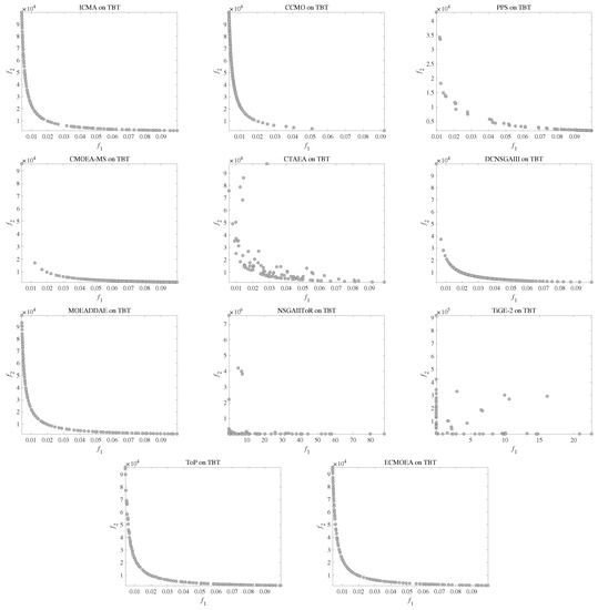
Figure A6.
Feasible and non-dominated solution sets obtained by ECMOEA and CMOEAs in comparison on Two Bar Truss Design problem with the median IGD value among 30 runs.
References
- Bani-Bakr, A.; Hindia, M.N.; Dimyati, K.; Hanafi, E.; Tengku Mohmed Noor Izam, T.F. Multi-Objective Caching Optimization for Wireless Backhauled Fog Radio Access Network. Symmetry 2021, 13, 708. [Google Scholar] [CrossRef]
- Wang, J.; Zhou, Y.; Wang, Y.; Zhang, J.; Chen, C.L.P.; Zheng, Z. Multiobjective Vehicle Routing Problems With Simultaneous Delivery and Pickup and Time Windows: Formulation, Instances, and Algorithms. IEEE Trans. Cybern. 2016, 46, 582–594. [Google Scholar] [CrossRef] [PubMed]
- Tan, B.; Ma, H.; Mei, Y.; Zhang, M. Evolutionary Multi-Objective Optimization for Web Service Location Allocation Problem. IEEE Trans. Serv. Comput. 2018, 14, 458–471. [Google Scholar] [CrossRef] [Green Version]
- Mnasri, S.; Nasri, N.; Van Den Bossche, A.; Val, T. 3D indoor redeployment in IoT collection networks: A real prototyping using a hybrid PI-NSGA-III-VF. In Proceedings of the 2018 14th International Wireless Communications Mobile Computing Conference (IWCMC), Limassol, Cyprus, 25–29 June 2018; pp. 780–785. [Google Scholar] [CrossRef]
- Zheng, A.; Li, B.; Zheng, M.; Zhong, H. Multi-Objective UAV Trajectory Planning in Uncertain Environment. Symmetry 2021, 13, 2160. [Google Scholar] [CrossRef]
- Su, Z.; Zhang, G.; Yue, F.; Zhan, D.; Li, M.; Li, B.; Yao, X. Enhanced Constraint Handling for Reliability-Constrained Multi-objective Testing Resource Allocation. IEEE Trans. Evol. Comput. 2021, 25, 537–551. [Google Scholar] [CrossRef]
- Li, X.; Zhu, X.; Li, B. Multi-Objective Optimization of Differentiated Urban Ring Road Bus Lines and Fares Based on Travelers Interactive Reinforcement Learning. Symmetry 2021, 13, 2301. [Google Scholar] [CrossRef]
- Ishibuchi, H.; Murata, T. A multi-objective genetic local search algorithm and its application to flowshop scheduling. IEEE Trans. Syst. Man Cybern. Part C (Appl. Rev.) 1998, 28, 392–403. [Google Scholar] [CrossRef]
- Wu, H.C. Using Shapley Values and Genetic Algorithms to Solve Multiobjective Optimization Problems. Symmetry 2021, 13, 2021. [Google Scholar] [CrossRef]
- Li, B.; Li, J.; Ke, T.; Xin, Y. Many-Objective Evolutionary Algorithms: A survey. ACM Comput. Surv. 2015, 48, 1–35. [Google Scholar] [CrossRef] [Green Version]
- Tian, Y.; Si, L.; Zhang, X.; Cheng, R.; He, C.; Tan, K.; Jin, Y. Evolutionary Large-Scale Multi-Objective Optimization: A Survey. ACM Comput. Surv. 2022, 54, 1–34. [Google Scholar] [CrossRef]
- Deb, K.; Pratap, A.; Agarwal, S.; Meyarivan, T. A fast and elitist multiobjective genetic algorithm: NSGA-II. IEEE Trans. Evol. Comput. 2002, 6, 182–197. [Google Scholar] [CrossRef] [Green Version]
- Zhang, Q.; Li, H. MOEA/D: A Multiobjective Evolutionary Algorithm Based on Decomposition. IEEE Trans. Evol. Comput. 2007, 11, 712–731. [Google Scholar] [CrossRef]
- Zitzler, E.; Künzli, S. Indicator-Based Selection in Multiobjective Search. In International Conference on Parallel Problem Solving from Nature; Springer: Berlin/Heidelberg, Germany, 2004. [Google Scholar]
- Yuan, J.; Liu, H.L.; Ong, Y.S.; He, Z. Indicator-based Evolutionary Algorithm for Solving Constrained Multi-objective Optimization Problems. IEEE Trans. Evol. Comput. 2021. [Google Scholar] [CrossRef]
- Zhu, Q.; Zhang, Q.; Lin, Q. A Constrained Multiobjective Evolutionary Algorithm With Detect-and-Escape Strategy. IEEE Trans. Evol. Comput. 2020, 24, 938–947. [Google Scholar] [CrossRef]
- Tian, Y.; Zhang, T.; Xiao, J.; Zhang, X.; Jin, Y. A Coevolutionary Framework for Constrained Multi-Objective Optimization Problems. IEEE Trans. Evol. Comput. 2020, 25, 102–116. [Google Scholar] [CrossRef]
- Ma, Z.; Wang, Y.; Song, W. A New Fitness Function With Two Rankings for Evolutionary Constrained Multiobjective Optimization. IEEE Trans. Syst. Man Cybern. Syst. 2019, 51, 5005–5016. [Google Scholar] [CrossRef]
- Jain, H.; Deb, K. An Evolutionary Many-Objective Optimization Algorithm Using Reference-Point Based Nondominated Sorting Approach, Part II: Handling Constraints and Extending to an Adaptive Approach. IEEE Trans. Evol. Comput. 2014, 18, 602–622. [Google Scholar] [CrossRef]
- Li, K.; Chen, R.; Fu, G.; Yao, X. Two-Archive Evolutionary Algorithm for Constrained Multiobjective Optimization. IEEE Trans. Evol. Comput. 2019, 23, 303–315. [Google Scholar] [CrossRef] [Green Version]
- Fan, Z.; Li, W.; Cai, X.; Huang, H.; Fang, Y.; Yugen, Y.; Mo, J.; Wei, C.; Goodman, E. An Improved Epsilon Constraint-handling Method in MOEA/D for CMOPs with Large Infeasible Regions. Soft Comput. 2019, 23, 12491–12510. [Google Scholar] [CrossRef] [Green Version]
- Fan, Z.; Li, W.; Cai, X.; Li, H.; Wei, C.; Zhang, Q.; Deb, K.; Goodman, E. Push and pull search for solving constrained multi-objective optimization problems. Swarm Evol. Comput. 2019, 44, 665–679. [Google Scholar] [CrossRef] [Green Version]
- Liu, Z.; Wang, Y. Handling Constrained Multiobjective Optimization Problems With Constraints in Both the Decision and Objective Spaces. IEEE Trans. Evol. Comput. 2019, 23, 870–884. [Google Scholar] [CrossRef]
- Liu, Z.Z.; Wang, B.C.; Tang, K. Handling Constrained Multiobjective Optimization Problems via Bidirectional Coevolution. IEEE Trans. Cybern. 2021, 1–14. [Google Scholar] [CrossRef]
- Tian, Y.; Zhang, Y.; Su, Y.; Zhang, X.; Tan, K.; Jin, Y. Balancing Objective Optimization and Constraint Satisfaction in Constrained Evolutionary Multi-Objective Optimization. IEEE Trans. Cybern. 2020. [Google Scholar] [CrossRef]
- Takahama, T.; Sakai, S. Constrained Optimization by the ε Constrained Differential Evolution with Gradient-Based Mutation and Feasible Elites. In Proceedings of the 2006 IEEE International Conference on Evolutionary Computation, Vancouver, BC, Canada, 16–21 July 2006; pp. 1–8. [Google Scholar] [CrossRef]
- Fan, Z.; Wang, Z.; Li, W.; Yuan, Y.; You, Y.; Yang, Z.; Sun, F.; Ruan, J. Push and pull search embedded in an M2M framework for solving constrained multi-objective optimization problems. Swarm Evol. Comput. 2020, 54, 100651. [Google Scholar] [CrossRef] [Green Version]
- Jiao, R.; Zeng, S.; Li, C.; Yang, S.; Ong, Y.S. Handling Constrained Many-Objective Optimization Problems via Problem Transformation. IEEE Trans. Cybern. 2020, 51, 4834–4847. [Google Scholar] [CrossRef] [PubMed]
- Tessema, B.; Yen, G.G. A Self Adaptive Penalty Function Based Algorithm for Constrained Optimization. In Proceedings of the 2006 IEEE International Conference on Evolutionary Computation, Vancouver, BC, Canada, 16–21 July 2006; pp. 246–253. [Google Scholar] [CrossRef]
- Jiao, L.; Luo, J.; Shang, R.; Liu, F. A modified objective function method with feasible-guiding strategy to solve constrained multi-objective optimization problems. Appl. Soft Comput. 2014, 14, 363–380. [Google Scholar] [CrossRef]
- Ming, M.; Trivedi, A.; Wang, R.; Srinivasan, D.; Zhang, T. A Dual-Population based Evolutionary Algorithm for Constrained Multi-Objective Optimization. IEEE Trans. Evol. Comput. 2021, 25, 739–753. [Google Scholar] [CrossRef]
- Ma, Z.; Wang, Y. Shift-Based Penalty for Evolutionary Constrained Multiobjective Optimization and Its Application. IEEE Trans. Cybern. 2021, 1–13. [Google Scholar] [CrossRef]
- Liu, Z.; Wang, Y.; Wang, B. Indicator-Based Constrained Multiobjective Evolutionary Algorithms. IEEE Trans. Syst. Man Cybern. Syst. 2019, 51, 5414–5426. [Google Scholar] [CrossRef]
- Zhou, Y.; Zhu, M.; Wang, J.; Zhang, Z.; Xiang, Y.; Zhang, J. Tri-Goal Evolution Framework for Constrained Many-Objective Optimization. IEEE Trans. Syst. Man Cybern. Syst. 2020, 50, 3086–3099. [Google Scholar] [CrossRef]
- Xiang, Y.; Yang, X.; Huang, H.; Wang, J. Balancing Constraints and Objectives by Considering Problem Types in Constrained Multiobjective Optimization. IEEE Trans. Cybern. 2021, 1–14. [Google Scholar] [CrossRef] [PubMed]
- Bader, J.; Zitzler, E. HypE: An Algorithm for Fast Hypervolume-Based Many-Objective Optimization. Evol. Comput. 2011, 19, 45–76. [Google Scholar] [CrossRef] [PubMed]
- Ishibuchi, H.; Imada, R.; Masuyama, N.; Nojima, Y. Comparison of Hypervolume, IGD and IGD+ from the Viewpoint of Optimal Distributions of Solutions. In Evolutionary Multi-Criterion Optimization; Springer: Cham, Switzerland, 2019; pp. 332–345. [Google Scholar]
- Tian, Y.; Cheng, R.; Zhang, X.; Jin, Y. PlatEMO: A MATLAB Platform for Evolutionary Multi-Objective Optimization. IEEE Comput. Intell. Mag. 2017, 12, 73–87. [Google Scholar] [CrossRef] [Green Version]
- Fan, Z.; Li, W.; Cai, X.; Li, H.; Wei, C.; Zhang, Q.; Deb, K.; Goodman, E. Difficulty Adjustable and Scalable Constrained Multiobjective Test Problem Toolkit. Evol. Comput. 2020, 28, 339–378. [Google Scholar] [CrossRef] [PubMed] [Green Version]
- Ma, Z.; Wang, Y. Evolutionary Constrained Multiobjective Optimization: Test Suite Construction and Performance Comparisons. IEEE Trans. Evol. Comput. 2019, 23, 972–986. [Google Scholar] [CrossRef]
- Tian, Y.; Cheng, R.; Zhang, X.; Su, Y.; Jin, Y. A Strengthened Dominance Relation Considering Convergence and Diversity for Evolutionary Many-Objective Optimization. IEEE Trans. Evol. Comput. 2019, 23, 331–345. [Google Scholar] [CrossRef] [Green Version]
- Caliński, T. Review of Principles and Procedures of Statistics: A Biometrical Approach, by R. G. D. Steel & J. H. Torrie. Biometrics 1981, 37, 859–860. [Google Scholar] [CrossRef]
- Derrac, J.; García, S.; Molina, D.; Herrera, F. A practical tutorial on the use of nonparametric statistical tests as a methodology for comparing evolutionary and swarm intelligence algorithms. Swarm Evol. Comput. 2011, 1, 3–18. [Google Scholar] [CrossRef]
- Agrawal, R.; Deb, K.; Agrawal, R. Simulated Binary Crossover for Continuous Search Space. Complex Syst. 2000, 9, 115–148. [Google Scholar]
- Alcalá-Fdez, J.; Sánchez, L.; García, S.; del Jesus, M.J.; Ventura, S.; Garrell, J.M.; Otero, J.; Romero, C.; Bacardit, J.; Rivas, V.M.; et al. KEEL: A software tool to assess evolutionary algorithms for data mining problems. Soft Comput. 2009, 13, 307–318. [Google Scholar] [CrossRef]
- Kumar, A.; Wu, G.; Ali, M.; Mallipeddi, R.; Suganthan, P.; Das, S. A test-suite of non-convex constrained optimization problems from the real-world and some baseline results. Swarm Evol. Comput. 2020, 56, 100693. [Google Scholar] [CrossRef]
- Hassanat, A.B.A. Two-point-based binary search trees for accelerating big data classification using KNN. PLoS ONE 2018, 13, e0207772. [Google Scholar] [CrossRef] [PubMed] [Green Version]
Publisher’s Note: MDPI stays neutral with regard to jurisdictional claims in published maps and institutional affiliations. |
© 2022 by the authors. Licensee MDPI, Basel, Switzerland. This article is an open access article distributed under the terms and conditions of the Creative Commons Attribution (CC BY) license (https://creativecommons.org/licenses/by/4.0/).