Addressing Class Overlap under Imbalanced Distribution: An Improved Method and Two Metrics

Abstract

Class imbalance, as a phenomenon of asymmetry, has an adverse effect on the performance of most machine learning and overlap is another important factor that affects the classification performance of machine learning algorithms. This paper deals with the two factors simultaneously, addressing the class overlap under imbalanced distribution. In this paper, a theoretical analysis is firstly conducted on the existing class overlap metrics. Then, an improved method and the corresponding metrics to evaluate the class overlap under imbalance distributions are proposed based on the theoretical analysis. A well-known collection of the imbalanced datasets is used to compare the performance of different metrics and the performance is evaluated based on the Pearson correlation coefficient and the $\xi$ correlation coefficient. The experimental results demonstrate that the proposed class overlap metrics outperform other compared metrics for the imbalanced datasets and the Pearson correlation coefficient with the AUC metric of eight algorithms can be improved by 34.7488% in average.

1. Introduction

Machine learning has been widely applied to solve problems in various fields. One of the common and important challenges in solving these problems by machine learning is the classification under imbalanced distribution [1]. The imbalance is encountered by a large number of applications where the concerned samples are rare, such as disease diagnosis, financial fraud detection, network intrusion detection, and so on [2]. The data distributions in these fields are asymmetry that the number of concerned positive samples are smaller than that of negative samples. Most standard classification algorithms are designed based on the concept of symmetry, relatively balanced class distribution or equal cost of misclassification [3]. The classification performances of these algorithms are degraded for handling the imbalance problem to some extent. Hence, building symmetry in machine learning for data under asymmetry distribution is an important research topic [4]. In [5], a novel class imbalance reduction algorithm is proposed to build a symmetry by considering distribution properties of the dataset to improve the performance in software defect prediction. In addition, there are also a lot of methods are proposed to handle the imbalance problem, which can be referred in [2,6].

Besides the imbalance, class overlap is also an important factor that affects the performance of classification [7]. In addition, the research of Liu et al. [8] demonstrated that the sample is often misclassified if it is in a class overlapping boundary. Oh [9] proposed the R value based on the ratio of overlapping areas to the whole dataset and the experimental results show that the R value is strongly correlated with the classification accuracy. In addition, Denil [10] has given a systematic analysis on the imbalance and overlap. The analysis shows that the overlap problem has a greater influence on classification performance than the imbalance in isolation and the classification performance is decreased significantly when the overlap and imbalance are both exist. To deal with the classification of datasets with class overlap and imbalance, some research works have also been conducted [7,11].

The classification methods for the datasets with class overlap and imbalance are important, but so are the quantitative estimation methods of the class overlap level for imbalanced datasets [9]. It can make contributions to understand the characteristic of the datasets and then help to design suitable methods for better classification performance. Klomsae et al. [12] adopts the R value to indicate the classification performance of the dataset and propose a string grammar fuzzy-possibilistic C-medians algorithm to handle the overlapping data problem. In addition, some methods based on the R value to conduct feature selection [13,14], feature construction [15] and data sampling [16] are proposed for achieving better classification performance. Later, Borsos et al. [17] analyzed the problem of the R value for estimating the overlap level of imbalanced datasets and extended the R value to the $R_{aug}$ value for imbalanced datasets. The experimental results demonstrate that the $R_{aug}$ value has a stronger correlation with the classification performance, and it can also achieve better performance in algorithm selection for better classification performance. In addition, some feature selection research works are also conducted based on the $R_{aug}$ value [18,19].

The $R_{aug}$ value has achieved great performance for addressing the class overlap under imbalanced distribution. However, the experimental results in [17] show that the absolute value of the Pearson correlation coefficients of the $R_{aug}$ with the classification performances are lower than 0.7 and the correlation coefficients are varied to different algorithms. Therefore, both correlation coefficients with the classification performances and the generalization ability for different classification algorithms need to be improved. For this purpose, a theoretical analysis on the existing class overlap metrics is firstly conducted and then an improved method is proposed to measure the class overlap for imbalanced datasets in this paper. Based on the proposed method, the R and $R_{aug}$ are extended to $ImR$ and $Im{R}_{aug}$ for better estimating the class overlap level for imbalanced datasets. The comparison experiments conducted on a well-known collection of imbalanced datasets and eight commonly used classification algorithms are adopted to obtain the classification performance. In addition, the performances of different overlap metrics are evaluated based on the Pearson correlation coefficient and the $\xi$ correlation coefficient with the classification performance. The experimental results demonstrate the excellent performances of the proposed metrics, which indicates the superiority of the proposed method.

The contributions of this paper can be summarized as follows:

• A theoretical analysis on the existing class overlap measure R value is presented.
• A novel method along with two metrics for estimating the class overlap of the imbalanced datasets is proposed based on the theoretical analysis.
• The proposed two class overlap metrics are verified to be in higher correlations with the classification performance of imbalanced datasets.

The rest of the paper is organized as follows. The existing overlap metrics, the R and $R_{aug}$ values, are introduced in Section 2. Section 3 presents a theoretical analysis on the R value. Then, an improved method and two corresponding overlap metrics for imbalanced datasets are proposed based on the theoretical analysis. In addition, Section 4 describes the information about the experiments, such as experiment setup, adopted datasets, and performance evaluation. The experimental results and discussions are given in Section 5. Finally, the conclusions are drawn in Section 6.

2. The Existing Overlap Metrics

To estimate the level of class overlap, there are two metrics, the R value and the $R_{aug}$ value. These two metrics are introduced in this section. Before introducing the two metrics, some notations are presented as follows:

• N: the number of the samples
• n: the number of the classes
• $C_l$: the set of samples belonging to class $l,l\in [1,n]$
• U: the set of all samples, $U=C_1\cup \dots \cup C_i\cup \dots \cup C_n$
• $x_i^l$: the $ith$ sample in $C_l$
• k-$NN(x_i^l,U-C_l)$: the set of samples in k-nearest neighbor samples of $x_i^l$ that belong to the class different from $C_l$
• $\lambda \left(z\right)$: a 0-1 function that returns 1 when $z>0$ and returns 0 otherwise
• $\theta$: a threshold value within the range [0, $k/2$]

2.1. The R Value

The original R value is proposed by Oh [9] based on the assumption that a sample from class $C_l$ is overlapped with other samples if the number of the samples that is in its k nearest neighbors and also belongs to a class rather than $C_l$ is at least $\theta +1$. In addition, the R values of class $C_l$ and the whole dataset f are defined as Equations (1) and (2), respectively:

$$\begin{array}{c}\hfill R\left(C_l\right)=\frac{1}{|C_l|}\sum _{i=1}^{|C_l|}\lambda \left(\right|k-NN(x_i^l,U-C_l)|-\theta )\end{array}$$

(1)

$$R\left(f\right)=\frac{1}{\left|U\right|}\sum _{l=1}^n\sum _{i=1}^{|C_l|}\lambda \left(\right|k-NN(x_i^l,U-C_l)|-\theta )$$

(2)

According to the definition, the R value can be considered as the ratio of samples in the overlapping area. The range of the R value is [0, 1]. In addition, there are two parameters, $k,\theta$ needed to be predefined to calculate the R value. According to [9], the R value is strongly correlated with the accuracy of Support Vector Machine (SVM), Artificial Neural Network (ANN), and K Nearest Neighbor (KNN) algorithms when $k=7$ and $\theta =3$. With this parameter setting, a sample is considered to be in the overlapping area if at least four samples in its seven nearest neighbors belong to another class.

2.2. The $R_{aug}$ Value

In [9], the results also show that the R value is most strongly correlated with the classification accuracy of the majority class. In addition, Borsos et al. [17] evaluated R value on some imbalanced data sets with different imbalanced ratios and the experiment results showed that R value is almost constant, while the classification performance decreases with a larger imbalance ratio (IR). Therefore, they conducted an analysis of the R value in a simple case with only two classes, the majority class and minority class. The majority class and minority class are denoted as $C_N$ and $C_P$, respectively. Then, the R value of the whole dataset can be calculated as Equation (3):

$$\begin{array}{cc}\hfill R& =\frac{1}{|C_N|+|C_P|}(\sum _{i=1}|C_N|\lambda \left(\right|k-NN(x_i^N,C_P)|-\theta )+\sum _{i=1}|C_P|\lambda \left(\right|k-NN(x_i^P,C_N)|-\theta ))\hfill \\ \hfill & =\frac{1}{|C_P|+|C_N|}\left(\right|C_N|·R\left(C_N\right)+|C_P|·R\left(C_P\right))\hfill \end{array}$$

(3)

By introducing the imbalance ratio $IR=|C_N|/|C_P|$ into Equation (3), the equation can be simplified as Equation (4):

$$R=\frac{1}{IR+1}(IR·R\left(C_N\right)+R\left(C_P\right))$$

(4)

As the weight of the R value of the majority class is IR, the R value of the whole dataset will be dominated by R value of the majority class when the dataset has a large IR. Actually, the sample in the majority class has a low probability to be recognized in the overlap area, while the sample in the minority class has a high probability. Therefore, the weight of the R value of the majority class should be smaller than that of the minority class. Based on this analysis, the augmented R value defined as Equation (5) is proposed by Borsos et al. [17]:

$$R_{aug}=\frac{1}{IR+1}(R\left(C_N\right)+IR·R\left(C_P\right))$$

(5)

It can be seen that the $R_{aug}$ value is dominated by the R value of the minority class for datasets with large IR, and it is equal to R value for balanced datasets with $IR=1$. The experimental results in [17] demonstrated that it could achieve a stronger correlation with the classification performance evaluated by the metric of the area under the Receiver Operating Characteristic (ROC) curve.

3. The Proposed Method and Corresponding Overlap Metrics

In this section, the theoretical analysis of the R value is firstly conducted. Then, an improved method to recognize the overlap area for imbalanced datasets is proposed and the corresponding overlap metrics are introduced.

3.1. Theoretical Analysis of the R Value

Consider a dataset with N samples $X=\{x_1,\dots ,x_i\dots ,x_N\}$, the number of samples in the same class with each sample $x_i$ is denoted as $r_i$. In the ideal non-overlapping data distribution, all samples are distributed very well so that the $r_i$ nearest samples of the sample $x_i$ along with the sample $x_i$ itself are all in the same class, while there may be some samples in the $r_i$ nearest samples of the sample $x_i$ that are in a different class to the class of $x_i$ in real data distribution.

Let’s keep it simple; only consider the $k_i$ nearest data samples $(k_i<r_i)$ of the sample $x_i$ in real data distribution. As shown in Figure 1, let $P_i$ be denoted as the set of $r_i$ nearest samples of the $x_i$ in the ideal data distribution, and $Q_i$ represents the set of $k_i$ nearest samples of the $x_i$ in the real data distribution. For any sample except $x_i$, it can be represented by $x^{TP}$, $x^{FP}$, $x^{FN}$, and $x^{TN}$. The meanings of these four kinds samples are presented as follows:

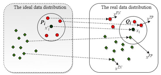
Figure 1. The comparison analysis of the data distribution.

• $x^{TP}$: the sample which is in both $P_i$ and $Q_i$
• $x^{TN}$: the sample in neither $P_i$ nor $Q_i$
• $x^{FN}$: the sample which is in $P_i$ but not in $Q_i$
• $x^{FP}$: the sample that are not in $P_i$ but in $Q_i$

Denote the number of $x^{TP}$ samples as $N_i^{TP}$, the number of $x^{FN}$ samples that as $N_i^{FN}$, the number of $x^{FP}$ samples that as $N_i^{FP}$ and the number of $x^{TN}$ samples that are as $N_i^{TN}$. According to the definition of R value, the contribution of the sample $x_i$ to the R value is determined by $N_i^{TP}$ and $N_i^{FP}$ as $k_i=N_i^{TP}+N_i^{FP}$. Actually, the contribution of $x_i$ to the R value can be determined based on the probability distribution. In the following, the contribution is analyzed based on the distance between the real data distribution and the ideal data distribution from the perspective of probability.

To measure the distance between distributions, the Kullback–Leibler (K-L) divergence is commonly used. In addition, to conduct the calculation of K-L divergence, denote $p_{j|i}$ and $q_{j|i}$ as the conditional probabilities of sample $x_j$ given $x_i$ for the ideal data distribution and the real data distribution. In addition, the conditional probability of the samples in the $P_i$ and $Q_i$ can be defined to be an equal non-zero probability and the conditional probability of the other samples can be defined to a near zero probability according to [20]. Then, the detailed conditional probabilities of $p_{j|i}$ and $q_{j|i}$ are shown in Equations (6) and (7):

$$p_{j|i}=\left\{\begin{array}{cc}\frac{1-\delta }{r_i}\hfill & ,if{x}_i\in P_i\hfill \\ \frac{\delta }{N-r_i-1}\hfill & ,otherwise\hfill \end{array}\right.$$

(6)

$$q_{j|i}=\left\{\begin{array}{cc}\frac{1-\delta }{k_i}\hfill & ,if{x}_i\in Q_i\hfill \\ \frac{\delta }{N-k_i-1}\hfill & ,otherwise\hfill \end{array}\right.$$

(7)

Based on the conditional probabilities, the distance, the K-L divergence $D(q_{j|i},p_{j|i})$, can be defined as Equation (8) shows. Due to the near zero value of $\delta$, the distance can be simplified to Equation (9). According to Equation (9), $N_i^{TP}$ and $N_i^{FP}$ dominate the distance, which is consistent with the definition of the R value:

$$\begin{array}{cc}\hfill D(q_{j|i},p_{j|i})& =\sum _{j\ne i,x_j\in P_i,x_j\in Q_i}(q_{j|i}log\frac{q_{j|i}}{p_{j|i}})+\sum _{j\ne i,x_j\in P_i,x_j\notin Q_i}(q_{j|i}log\frac{q_{j|i}}{p_{j|i}})\hfill \\ \hfill & +\sum _{j\ne i,x_j\notin P_i,x_j\in Q_i}(q_{j|i}log\frac{q_{j|i}}{p_{j|i}})+\sum _{j\ne i,x_j\notin P_i,x_j\notin Q_i}(q_{j|i}log\frac{q_{j|i}}{p_{j|i}})\hfill \end{array}$$

(8)

$$\begin{array}{c}\hfill D(q_{j|i},p_{j|i})\approx N_i^{TP}\{\frac{1-\delta }{k_i}log\left(\frac{1-\delta }{k_i}\frac{r_i}{1-\delta }\right)\}+N_i^{FP}\{\frac{1-\delta }{k_i}log\left(\frac{1-\delta }{k_i}\frac{N-r_i-1}{\delta }\right)\}\end{array}$$

(9)

Equation (9) can be further simplified to Equation (10) because of the near zero value of $\delta$. It can be seen that the distance actually is dominated by the ratio of $N_i^{FP}$ and $k_i(k_i=N_i^{FP}+N_i^{TP})$. Therefore, a reasonable threshold for judging whether $x_i$ has a contribution to the R value is 0.5. If $N_i^{FP}/k_i>0.5$, it indicates that $x_i$ is in the overlap area. For $k_i=7$, if $N_i^{FP}/k_i>0.5$, $N_i^{FP}$ should be at least 4. It is consistent with the implementation of the R value in the experiments of [9]:

$$\begin{array}{cc}\hfill D(q_{j|i},p_{j|i})& \approx \frac{N_i^{TP}}{k_i}(1-\delta )log\frac{r_i}{k_i}+\frac{N_i^{FP}}{k_i}(1-\delta )(log\frac{1-\delta }{\delta }+log\frac{N-r_i-1}{k_i})\hfill \\ \hfill & \approx \frac{N_i^{FP}}{k_i}(1-\delta )log\frac{1-\delta }{\delta }\hfill \end{array}$$

(10)

In addition, the sample $x_i$ is correctly classified to a class if $N_i^{TP}>N_i^{FP}$ in the k nearest neighbor for the KNN algorithm, which is contrary to the definition of the R value. Therefore, the R value can be strongly and negatively correlated with the accuracy of the KNN algorithm.

3.2. The Proposed Method

From the above theoretical analysis, it can be seen that the class overlap is actually not only determined by $N_i^{FP}$ but also $N_i^{TP}$, while the contribution of $N_i^{TP}$ is ignored for the R value. As Equation (10) shows, it can be omitted as the coefficient $log\frac{r_i}{k_i}$ is constant for balanced data sets with the same $k_i$ for all samples. However, when the same $k_i$ is adopted, the coefficient is varied from different classes due to the different $r_i$ for imbalanced data sets. To make the coefficients of $N_i^{TP}$ equal for different classes in an imbalanced dataset, the condition shown in Equation (11) should be satisfied. Then, Equation (12) can be obtained. Besides, the same result will be obtained if the deduction is conducted based on Hellinger distance, which can be found in Appendix A. It indicates that the adopted value of k should be in proportion to the number of samples in the class and the smaller value of $k_{min}$ should be adopted for the minority class:

$$log\frac{r_N}{k_N}=log\frac{r_P}{k_P}$$

(11)

$$\frac{k_N}{k_P}=\frac{r_N}{r_P}=IR$$

(12)

According to Equation (12), if k is used for the majority class, $\lceil k/IR\rceil$ should be used for the minority class as it must be a positive integer. Based on this analysis, an improved method to calculate the overlap of different classes is proposed as Equation (13) shows, where $C_N$ is the number of samples in the majority class. In this way, the samples in the minority class will not be considered in an overlap area easily:

$$R\left(C_l\right)=\frac{1}{|C_l|}\sum _{i=1}^{|C_l|}\lambda \left(\right|\lceil \frac{k·|C_l|}{|C_N|}\rceil -NN(x_i^l,U-C_l)|-\theta ))$$

(13)

An intuitive demonstration of how the proposed method works is presented in Figure 2. For the sample $x_i^N$ in the majority class, both $k=3$ and $k=5$ are suitable to decide whether $x_i^N$ is in the class overlap region or not, while the sample $x_i^P$ in the minority class will be recognized to be in the overlap region when $k=5$. When $k=3=\lceil 5/2\rceil$, the $x_i^P$ can be correctly recognized to be in the non-overlap region.

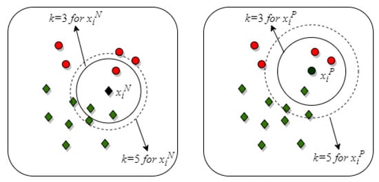
Figure 2. An intuitive demonstration of how the proposed method works.

3.3. The Proposed Metrics

According to the proposed method, two improved overlap metrics based on the R and $R_{aug}$ for binary imbalance datasets can be introduced. The two metrics, denoted as $ImR$ and $Im{R}_{aug}$, are defined as Equations (14) and (15):

$$\begin{array}{cc}\hfill ImR& =\frac{1}{IR+1}(IR·R\left(C_N\right)+R\left(C_P\right))\hfill \\ \hfill & =\frac{1}{|C_N|+|C_P|}(\sum _{i=1}^{|C_N|}\lambda \left(\right|k-NN(x_i^N,C_P)|-\theta )+\sum _{i=1}^{|C_P|}\lambda \left(\right|\lceil \frac{k}{IR}\rceil -NN(x_i^P,C_N)|-\theta ))\hfill \end{array}$$

(14)

$$\begin{array}{cc}\hfill Im{R}_{aug}& =\frac{1}{IR+1}(R\left(C_N\right)+IR·R\left(C_P\right))\hfill \\ \hfill & =\frac{1}{|C_N|+|C_P|}(\frac{1}{IR}\sum _{i=1}^{|C_N|}\lambda \left(\right|k-NN(x_i^N,C_P)|-\theta )+IR\sum _{i=1}^{|C_P|}\lambda \left(\right|\lceil \frac{k}{IR}\rceil -NN(x_i^P,C_N)|-\theta ))\hfill \end{array}$$

(15)

According to the definition of the two metrics, they can both be equal to the original R value when the dataset is balanced ($IR=1$). In addition, the experimental results in [9,17] demonstrate that the R and $R_{aug}$ are strongly correlated with the accuracy and the area under the ROC curve (AUC) respectively. Therefore, it is expected that $ImR$ is more strongly correlated with the accuracy of the imbalanced datasets and $Im{R}_{aug}$ is more strongly correlated with the AUC of the imbalanced datasets.

4. Experiment Design

In this section, the experiment setup is firstly introduced. Then, the datasets adopted in the experiments are presented. Finally, the evaluation metric for the comparison of different class overlap metrics is described.

4.1. Experiment Setup

The experiments are conducted to prove the effectiveness of the proposed method and the two metrics for addressing the class overlap of the imbalanced datasets. To evaluate the effectiveness, not only the correlation of different overlap metrics with the classification performance but also the time consuming of the overlap metrics and the classification modeling are compared. The Pearson correlation coefficient and the $\xi$ correlation coefficient are adopted to obtain the correlation result. The Pearson correlation coefficient can only handle the linear correlations, while the $\xi$ correlation coefficient can deal with both the linear and nonlinear correlations.

According to the investigation of Guo et al. in [2], the AUC and accuracy are the most frequently used metrics for evaluating the classification performance. The AUC is obtained based on the ROC curve which consists of a series points of (false positive rate, true positive rate) [21]. In addition, the points are generated by varying different thresholds for the prediction probability of the classifier. As the AUC is robust to the imbalanced datasets [22], it is recognized as an objective metric and widely utilized to evaluate the classification performance for imbalanced problems. The accuracy is defined as the rate of the number of correctly predicted samples to the number of samples in the whole dataset. Although the accuracy has been proved to be biased to the majority class, it is still frequently used in the research on imbalance learning as it is the most general and intuitive metric [2]. In addition, the proposed metrics $ImR$ and $Im{R}_{aug}$ are expected to be strongly correlated with the accuracy and AUC respectively based on the analysis in Section 3. Therefore, the two metrics are both adopted to evaluate the classification performance for the better evaluation of the proposed overlap metrics.

Moreover, for the comparison of the generalization ability, eight commonly used algorithms are adopted to obtain the classification performance and the performances are obtained based on the 5-fold cross validation. The eight classification algorithms are k-nearest neighbor (KNN), Naive Bayesian (NB), Support Vector Machine with linear kernel (SVM-L), Support Vector Machine with radial basis kernel (SVM-R), Decision Tree (DT), Multiple Layer Perceptron (MLP), Random Forest (RF), and Adaptive Boosting (AdaB). All methods in the experiments are implemented in python based on some packages like scikit-learn [23] and so on. The parameters of the eight classification algorithms are set to default in the experiment. In addition, the same parameter setting, $k=7,\theta =k/2$, is adopted for all overlap metrics.

4.2. Datasets

In the experiments, a relatively well-known collection of 66 datasets for imbalanced classification is utilized. This collection can be obtained from the KEEL repository and has been adopted in [17,24]. The descriptions of these datasets are shown in Table 1, where #Inst. and #Attrs indicate the number of samples and attributes, respectively, and $IR$ means the imbalance ratio. The imbalance ratios of the datasets are in a very wide range. The minimum imbalance ratio is 1.82, while the maximum imbalance ratio is 128.87.

Table 1. The information about the imbalanced datasets.

Dataset	#Inst.	#Attrs	IR	Dataset	#Inst.	#Attrs	IR
Glass1	214	9	1.82	Glass04vs5	92	9	9.22
Ecoli0vs1	220	7	1.86	Ecoli0346vs5	205	7	9.25
Wisconsin	683	9	1.86	Ecoli0347vs56	257	7	9.28
Pima	768	8	1.9	Yeast05679vs4	528	8	9.35
Iris0	150	4	2	Ecoli067vs5	220	6	10
Glass0	214	9	2.06	Vowel0	988	13	10.1
Yeast1	1484	8	2.46	Glass016vs2	192	9	10.29
Vehicle1	846	18	2.52	Glass2	214	9	10.39
Vehicle2	846	18	2.52	Ecoli0147vs2356	336	7	10.59
Vehicle3	846	18	2.52	Led7digit02456789vs1	443	7	10.97
Haberman	306	3	2.68	Glass06vs5	108	9	11
Glass0123vs456	214	9	3.19	Ecoli01vs5	240	6	11
Vehicle0	846	18	3.23	Glass0146vs2	205	9	11.06
Ecoli1	336	7	3.36	Ecoli0147vs56	332	6	12.28
New-thyroid2	215	5	4.92	Cleveland0vs4	177	13	12.62
New-thyroid1	215	5	5.14	Ecoli0146vs5	280	6	13
Ecoli2	336	7	5.46	Ecoli4	336	7	13.84
Segment0	2308	19	6.01	Yeast1vs7	459	8	13.87
Glass6	214	9	6.38	Shuttle0vs4	1829	9	13.87
Yeast3	1484	8	8.11	Glass4	214	9	15.47
Ecoli3	336	7	8.19	Page-blocks13vs2	472	10	15.85
Page-blocks0	5472	10	8.77	Abalone9vs18	731	8	16.68
Ecoli034vs5	200	7	9	Glass016vs5	184	9	19.44
Yeast2vs4	514	8	9.08	Shuttle2vs4	129	9	20.5
Ecoli067vs35	222	7	9.09	Yeast1458vs7	693	8	22.1
Ecoli0234vs5	202	7	9.1	Glass5	214	9	22.81
Glass015vs2	172	9	9.12	Yeast2vs8	482	8	23.1
Yeast0359vs78	506	8	9.12	Yeast4	1484	8	28.41
Yeast02579vs368	1004	8	9.14	Yeast1289vs7	947	8	30.56
Yeast0256vs3789	1004	8	9.14	Yeast5	1484	8	32.78
Ecoli046vs5	203	6	9.15	Ecoli0137vs26	281	7	39.15
Ecoli01vs235	244	7	9.17	Yeast6	1484	8	39.15
Ecoli0267vs35	224	7	9.18	Abalone19	4174	8	128.87

4.3. Evaluation of Correlation

Pearson correlation coefficient [25] is defined to measure the strength of the relationship between two variables in statistics. The equation of Pearson correlation coefficient is shown in Equation (16), where X and Y are two variables, $\overline{X}$ and $\overline{Y}$ are the mean value of the two variables, $cov(.,.)$ is the covariance, and $\sigma$ is the standard deviation:

$${\rho }_{X,Y}=\frac{cov(X,Y)}{{\sigma }_X{\sigma }_Y}=\frac{{\sum }_{i=1}^n(X_i-\overline{X})(Y_i-\overline{Y})}{\sqrt{{\sum }_{i=1}^n{(X_i-\overline{X})}^2}\sqrt{{\sum }_{i=1}^n{(Y_i-\overline{Y})}^2}}$$

(16)

The Pearson correlation coefficient is widely utilized to calculate the linear correlation of two variables. It has been used to compare the performance of R and $R_{aug}$ in [17], and it is also used in the experiments of this paper. In addition, the range of Pearson correlation coefficient $\rho$ is [−1, 1]. The bigger of the absolute value of $\rho$, the stronger correlation of the two variables. $\rho =1$ indicates that there is a perfect positive correlation between the two variables, while $\rho =-1$ means a perfect negative correlation. In addition, when $\rho =0$, it indicates that the two variables are dependent and there is no correlation can be found between them.

To further verify the linear correlation of the proposed metrics and the classification performance, the probabilities of the Pearson correlation results are also compared. The probability can be indicated by p-value, where the smaller p-value indicates the stronger support for the result of Pearson correlation coefficient. Generally, a p-value smaller than 0.05 means that the result of linear correlation is solid. In addition, the result is significantly solid when the p-value is smaller than 0.01.

Besides the Pearson correlation coefficient, the $\xi$ correlation coefficient is also used to the evaluate the relationships of different overlap metrics with the classification performance. $\xi$ correlation coefficient, which was proposed in [26], can not only measure the linear correlation but also the nonlinear correlation. To calculate the $\xi$ correlation coefficient of a pair of variables (X, Y), the data should be rearranged as $(X_1,Y_1),\dots ,(X_n,Y_n)$ such that $X_1\le$··· $\le X_n$. Let $h_i$ be the number of j such that $Y_j\le Y_i$ and $l_i$ are the number of j such that $Y_j\ge Y_i$, and the $\xi$ correlation coefficient is defined as Equation (17) shown. It is in range of $[0,1]$, where $\xi (X,Y)=0$ indicates that X and Y are independent and $\xi (X,Y)=1$ indicates that Y is a measurable function of X:

$$\xi (X,Y)=1-\frac{n{\sum }_{i=1}^{n-1}|h_{i+1}-h_i|}{2{\sum }_{i=1}^n{l}_i(n-l_i)}$$

(17)

5. Results and Discussion

To verify the efficiency of the proposed method to measure class overlap, both the correlation results of different metrics with the AUC and the accuracy are compared. As the AUC metric is more objective than the accuracy for imbalance learning, the comparison of the correlations of different overlap metrics and the AUC of different algorithms is firstly conducted. In addition, then the correlation results of different metrics with the accuracy are compared. Finally, the overall results are summarized.

5.1. The Correlation Results for the AUC Metric

Figure 3 shows the correlation results of different overlap metrics with the AUCs of classification algorithms. The results demonstrate that the $Im{R}_{aug}$ metric achieved the best performance among these metrics for all classification algorithms. In addition, the $ImR$ metric also obtained better performance than the original R metric based on the AUC metric of classification algorithms. In addition, both the original R and $R_{aug}$ value have low correlation coefficients with the AUC of the NB algorithm. It can be seen that the generalization ability of the existing overlap metrics is not good. While, the correlation coefficients of the R and $R_{aug}$ with the NB algorithm are both largely improved by the proposed method. The $ImR$ and $Im{R}_{aug}$ seem to have better generalization abilities for these algorithms than the R and $R_{aug}$, respectively.

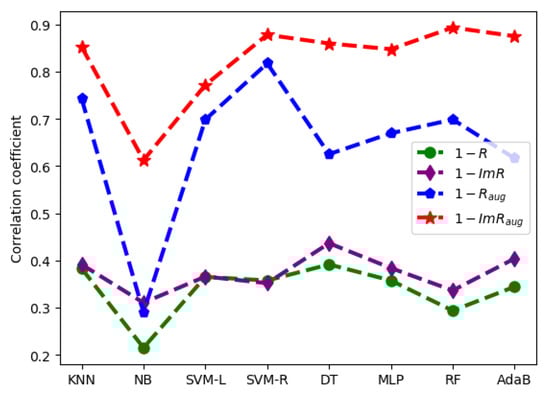
Figure 3. The Pearson correlation comparison between different overlap metrics and the AUCs of different algorithms on all data sets.

As expected, the $R_{aug}$ and $Im{R}_{aug}$ achieve much stronger correlations with the AUC of different algorithms. It is consistent with the result in [17]. In the following, the detailed correlation results of the $R_{aug}$ and $Im{R}_{aug}$ with different classification algorithms are compared. The detailed correlation coefficients along with the p-values of $R_{aug}$ and $Im{R}_{aug}$ with the AUC of different algorithms are presented in Table 2. It can be seen that the correlation coefficients of the $R_{aug}$ with the AUC of the DT, MLP, RF, and AdaB algorithms are all lower than 0.7, while the correlation coefficients with the AUC of these algorithms are all improved to more than 0.8 by $Im{R}_{aug}$. On average, the $Im{R}_{aug}$ achieves a 34.7488% improvement to the $R_{aug}$. An illustration of the correlation coefficient improvements of $Im{R}_{aug}$ over $R_{aug}$ is shown in Figure 4. The correlation coefficient between $R_{aug}$ and the AUC of the NB algorithm is largely improved by the proposed $Im{R}_{aug}$.

Table 2. The detailed Pearson correlation coefficient results of $R_{aug}$ and $Im{R}_{aug}$ with the AUCs of different algorithms on all data sets.

Algorithm	${\mathit{R}}_{\mathit{aug}}$	${\mathit{ImR}}_{\mathit{aug}}$	$\mathit{Improvement}$
KNN	−0.7425 ($9.62\times {10}^{-13}$)	−0.8525 ($\mathbf{1.09}\times {\mathbf{10}}^{-\mathbf{19}}$)	14.8108%
NB	−0.2900 ($1.82\times {10}^{-02}$)	−0.6125 ($\mathbf{4.60}\times {\mathbf{10}}^{-\mathbf{08}}$)	111.2128%
SVM-L	−0.6985 ($7.03\times {10}^{-11}$)	−0.7718 ($\mathbf{3.30}\times {\mathbf{10}}^{-\mathbf{14}}$)	10.5068%
SVM-R	−0.8176 ($5.48\times {10}^{-17}$)	−0.8783 ($\mathbf{3.51}\times {\mathbf{10}}^{-\mathbf{22}}$)	7.4199%
DT	−0.6253 ($2.00\times {10}^{-08}$)	−0.8598 ($\mathbf{2.38}\times {\mathbf{10}}^{-\mathbf{20}}$)	37.5162%
MLP	−0.6695 ($7.94\times {10}^{-10}$)	−0.8477 ($\mathbf{2.81}\times {\mathbf{10}}^{-\mathbf{19}}$)	26.6104%
RF	−0.6986 ($6.92\times {10}^{-11}$)	−0.8936 ($\mathbf{5.99}\times {\mathbf{10}}^{-\mathbf{24}}$)	27.9070%
AdaB	−0.6163 ($3.62\times {10}^{-08}$)	−0.8752 ($\mathbf{7.49}\times {\mathbf{10}}^{-\mathbf{22}}$)	42.0063%
Mean	−0.6448 (-)	−0.8239 (-)	34.7488%
SD	0.1571 (-)	0.0930 (-)	-

The bold values means better results and the values in the brackets are the p-value.

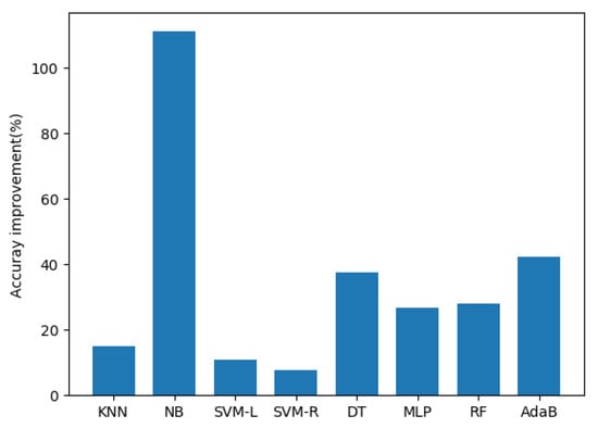
Figure 4. Correlation coefficient improvements of the $Im{R}_{aug}$ over the $R_{aug}$ with the AUCs of different algorithms on all datasets.

In addition, all the p-values of $Im{R}_{aug}$ are far less than 0.01, which indicates that $Im{R}_{aug}$ does have linear correlations with the AUC of these algorithms. In addition, the p-values of $Im{R}_{aug}$ are also much less than that of $R_{aug}$. Therefore, the $Im{R}_{aug}$ has a much better performance than the $R_{aug}$ for estimating the level of class overlap under imbalanced distribution. Moreover, $Im{R}_{aug}$ can not only achieve the better mean value of correlations with the AUCs of all classification algorithms, but also achieve the smaller standard deviation. It demonstrates that $Im{R}_{aug}$ also has a better generalization ability to these algorithms.

Figure 5 demonstrates the $\xi$ correlation coefficients of the AUCs of different algorithms with the $R_{aug}$ and $Im{R}_{aug}$. It can be seen that the result of the $\xi$ correlation coefficient is similar to the result of the Pearson correlation coefficient. The $x_i$ correlation coefficient of the AUC of the RF algorithm with the $Im{R}_{aug}$ is the highest and the correlation coefficient of the NB algorithm with $R_{aug}$ is largely improved by $Im{R}_{aug}$. In addition, the $\xi$ correlation coefficients of the AUCs of different algorithms with the $Im{R}_{aug}$ are all higher than that with the $R_{aug}$. Therefore, the comparison of $\xi$ correlation coefficient also demonstrates the superior of $Im{R}_{aug}$.

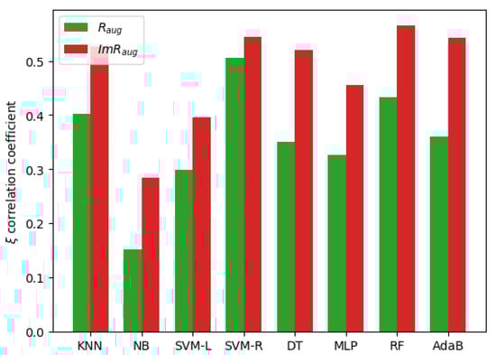
Figure 5. $\xi$ Correlation coefficients of the AUCs of different algorithms with the $R_{aug}$ and $Im{R}_{aug}$.

5.2. The Correlation Results for the Accuracy Metric

Figure 6 shows the correlation results of R and $ImR$ with the accuracy of several classification algorithms. It can be seen that the $ImR$ achieves better performance than the original R for more classification algorithms. In addition, the $Im{R}_{aug}$ measure also obtained better performance than the $R_{aug}$ measure based on the accuracy of classification algorithms.

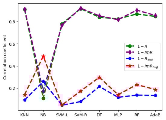
Figure 6. The correlation comparison of different overlap metrics and classification accuracies of different algorithms on all datasets.

The detailed correlation coefficients and p-values of the R and $ImR$ with the accuracy of different algorithms are shown in Table 3. As expected, the $ImR$ is strongly correlated with the accuracy of the KNN algorithm. The Pearson correlation coefficient of the $ImR$ with the accuracy of the KNN algorithm is more than 0.9. In addition, the $ImR$ also achieves high correlation coefficients with the accuracy of the SVM-R, DT, MLP, RF, and AdaB algorithms. Although the correlation coefficients of the R and $ImR$ with the accuracy of the NB algorithm are very low, the correlation coefficient is greatly improved by the $ImR$. On average, the $ImR$ achieves a 8.0898% improvement of the Pearson correlation coefficient to the R. Therefore, the $ImR$ has a better performance than the R for estimating the level of class overlap under imbalanced distribution.

Table 3. The detailed Pearson correlation coefficient results of R and $ImR$ with the accuracies of different algorithms on all data sets.

Algorithm	R	ImR	Improvement
KNN	−0.9085 ($6.11\times {10}^{-26}$)	−0.9125 ($\mathbf{1.53}\times {\mathbf{10}}^{-\mathbf{26}}$)	0.4441%
NB	−0.1091 ($3.83\times {10}^{-01}$)	−0.1742 ($\mathbf{1.62}\times {\mathbf{10}}^{-\mathbf{01}}$)	59.6436%
SVM-L	−0.7787 ($\mathbf{1.40}\times {\mathbf{10}}^{-\mathbf{14}}$)	−0.7674 ($5.67\times {10}^{-14}$)	−1.4452%
SVM-R	−0.9145 ($7.76\times {10}^{-27}$)	−0.9192 ($\mathbf{1.33}\times {\mathbf{10}}^{-\mathbf{27}}$)	0.5234%
DT	−0.8376 ($1.86\times {10}^{-18}$)	−0.8498 ($\mathbf{1.84}\times {\mathbf{10}}^{-\mathbf{19}}$)	1.4656%
MLP	−0.8229 ($\mathbf{2.31}\times {\mathbf{10}}^{-\mathbf{17}}$)	−0.8160 ($7.05\times {10}^{-17}$)	−0.8434
RF	−0.8672 ($4.77\times {10}^{-21}$)	−0.9014 ($\mathbf{6.04}\times {\mathbf{10}}^{-\mathbf{25}}$)	3.9400%
AdaB	−0.8451 ($4.56\times {10}^{-19}$)	−0.8535 ($\mathbf{8.83}\times {\mathbf{10}}^{-\mathbf{20}}$)	0.9902%
Mean	−0.7393 (-)	−0.7545 (-)	8.0898%
SD	0.2809 (-)	0.2609 (-)	-

The bold values means better results and the values in the brackets are the p-value.

In addition, all the p-values of $ImR$ except for the NB algorithm are far less than 0.01, which indicates that $ImR$ does have linear correlations with the ACC of most algorithms. In addition, the p-values of $ImR$ except for SVM-L and MLP algorithms are much less than that of R. Therefore, the $ImR$ has a much better performance than the R for estimating the level of class overlap under imbalanced distribution. Moreover, $ImR$ can not only achieve the better mean value of correlation coefficients with the accuracy of all classification algorithms, but also achieve the smaller standard deviation. It demonstrates that $ImR$ also has a better generalization ability to these algorithms.

Figure 7 presents the $\xi$ correlation coefficients of the accuracies of different algorithms with the $R_{aug}$ and $Im{R}_{aug}$. It can be seen that the result of the $\xi$ correlation coefficient is also similar to the result of the Pearson correlation coefficient. The $x_i$ correlation coefficient of the accuracy of the NB algorithm with the R is much smaller than that of the accuracies of other algorithms with the R, and the coefficient is largely improved by the $ImR$. The $x_i$ correlation coefficient of the accuracy of the SVM-R algorithm with the $ImR$ is also the highest. Meanwhile, the $\xi$ correlation coefficients of the accuracies of different algorithms with the $ImR$ are all higher than that with the R. Therefore, the comparison of $\xi$ correlation coefficient also shows that the $ImR$ has a better performance than that of the R.

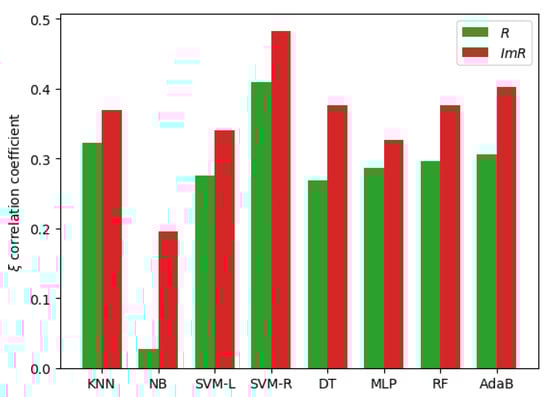
Figure 7. $\xi$ correlation coefficients of the accuracies of different algorithms with the R and $ImR$.

5.3. The Comparison of Time Consumption

The average time-consuming comparison of different overlap metrics and 5-fold cross validation of different classification algorithms is shown in Figure 8. It can be seen that the MLP algorithm has the most time-consuming performance due to the backpropagation. In addition, the RF and AdaB algorithms are also very time consuming because of the ensemble learning. In addition, these overlap metrics have a similar time consuming performance and the consuming time of the KNN algorithm is approximately four times that of the overlap metric. The main reason is that the k-nearest neighbors searching is the most time-consuming process for these overlap metrics and the KNN algorithm. The searching process will be conducted in the range of n samples for a dataset, and it will be conducted five times in the range of $\frac{4n}{5}$ samples for the 5-fold cross validation of the KNN algorithm. Therefore, the result is consistent to the analysis and the proposed overlap metrics are also superior in terms of time consumption.

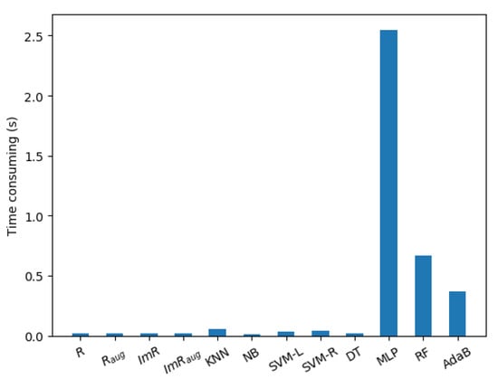
Figure 8. The average time-consuming comparison of different overlap metrics and 5-fold cross validation of different algorithms.

To sum up, the metrics $ImR$ and $Im{R}_{aug}$, which are proposed based on the proposed method, can achieve better performance than the original R and $R_{aug}$ respectively for estimating the level of class overlap of imbalanced datasets. Therefore, the conclusion that the proposed method and metrics are superior to address the class overlap under imbalanced distribution can be drawn.

6. Conclusions

In this paper, a theoretical analysis is conducted on the existing class overlap metrics and an improved method to address the class overlap under imbalanced distribution is proposed based on the theoretical analysis. Then, the corresponding metrics for estimating the class overlap of imbalanced datasets are also introduced. A well-known collection of the imbalanced datasets is used to compare the Pearson correlation coefficients and the $\xi$ correlation coefficients of different overlap metrics with the classification performance. In addition, the experimental results demonstrate that the proposed data overlap metrics outperform other compared metrics for the imbalanced datasets. The Pearson correlation coefficients with the AUC metric and the accuracy metric can be improved by 34.7488% and 8.0898% on average, respectively. Therefore, the proposed method and metrics can much better estimate the class overlap under imbalanced distribution.

In the future, the proposed metrics can be applied to feature selection and feature construction. In addition, they can also be used as meta-features in meta-learning for algorithm selection and parameters optimization.

References

- Japkowicz, N.; Stephen, S. The class imbalance problem: A systematic study. Intell. Data Anal. 2002, 6, 429–449. [Google Scholar] [CrossRef]
- Guo, H.; Li, Y.; Jennifer, S.; Gu, M.; Huang, Y.; Gong, B. Learning from class-imbalanced data: Review of methods and applications. Expert Syst. Appl. 2017, 73, 220–239. [Google Scholar]
- Sun, Y.; Wong, A.K.C.; Kamel, M.S. Classification of imbalanced data: A review. Int. J. Pattern Recognit. Artif. Intell. 2009, 23, 687–719. [Google Scholar] [CrossRef]
- Dogo, E.M.; Nwulu, N.I.; Twala, B.; Aigbavboa, C. Accessing Imbalance Learning Using Dynamic Selection Approach in Water Quality Anomaly Detection. Symmetry 2021, 13, 818. [Google Scholar] [CrossRef]
- Bejjanki, K.K.; Gyani, J.; Gugulothu, N. Class Imbalance Reduction (CIR): A Novel Approach to Software Defect Prediction in the Presence of Class Imbalance. Symmetry 2020, 12, 407. [Google Scholar] [CrossRef] [Green Version]
- He, H.; Garcia, E.A. Learning from Imbalanced Data. IEEE Trans. Knowl. Data Eng. 2009, 21, 1263–1284. [Google Scholar]
- Xiong, H.; Wu, J.; Liu, L. Classification with Class Overlapping: A Systematic Study. In Proceedings of the 1st International Conference on E-Business Intelligence (ICEBI 2010), Guangzhou, China, 19–21 December 2010; Atlantis Press: Dordrecht, The Netherlands, 2010; pp. 491–497. [Google Scholar]
- Liu, C.L. Partial discriminative training for classification of overlapping classes in document analysis. Int. J. Doc. Anal. Recognit. 2008, 11, 53–56. [Google Scholar] [CrossRef]
- Oh, S. A new dataset evaluation method based on category overlap. Comput. Biol. Med. 2011, 41, 115–122. [Google Scholar] [CrossRef]
- Denil, M.; Trappenberg, T. Overlap versus imbalance. In Advances in Artificial Intelligence; Canadian AI 2010. Lecture Notes Computer Science; Farzindar, A., Keselj, V., Eds.; Springer: Berlin/Heidelberg, Germany, 2010; Volume 6085, pp. 220–231. [Google Scholar]
- Lee, H.K.; Kim, S.B. An overlap-sensitive margin classifier for imbalanced and overlapping data. Expert Syst. Appl. 2018, 98, 72–83. [Google Scholar] [CrossRef]
- Klomsae, A.; Auephanwiriyakul, S.; Theera-Umpon, N. A string grammar fuzzy-possibilistic c-medians. Appl. Soft Comput. 2017, 57, 684–695. [Google Scholar] [CrossRef]
- Lee, J.; Batnyam, N.; Oh, S. RFS: Efficient feature selection method based on R-value. Comput. Biol. Med. 2013, 43, 91–99. [Google Scholar] [CrossRef]
- Wang, X.; Lin, X.; Huang, X.; Yang, Y. Ensemble unsupervised feature selection based on permutation and R-value. In Proceedings of the 2015 12th International Conference on Fuzzy Systems and Knowledge Discovery (FSKD), Zhangjiajie, China, 15–17 August 2015. [Google Scholar]
- Li, Z.; He, J.; Zhang, X.; He, J.; Qin, J. Toward high accuracy and visualization: An interpretable feature extraction method based on genetic programming and non-overlap degree. In Proceedings of the 2020 IEEE International Conference on Bioinformatics and Biomedicine (BIBM), Seoul, Korea, 16–19 December 2020; pp. 299–304. [Google Scholar]
- Kang, D.; Oh, S. Balanced Training/Test Set Sampling for Proper Evaluation of Classification Models. Intell. Data Anal. 2020, 24, 5–18. [Google Scholar] [CrossRef]
- Borsos, Z.; Lemnaru, C.; Potolea, R. Dealing with overlap and imbalance: A new metric and approach. Pattern Anal. Appl. 2018, 21, 381–395. [Google Scholar] [CrossRef]
- Fu, G.; Wu, Y.; Zong, M.; Yi, L. Feature selection and classification by minimizing overlap degree for class-imbalanced data in metabolomics. Chemom. Intell. Lab. Syst. 2020, 196, 103906. [Google Scholar] [CrossRef]
- Fatima, E.B.; Omar, B.; Abdelmajid, E.M.; Rustam, F.; Mehmood, A.; Choi, G.S. Minimizing the overlapping degree to improve class-imbalanced learning under sparse feature selection. Application to fraud detection. IEEE Access 2021, 9, 28101–28110. [Google Scholar] [CrossRef]
- Venna, J.; Peltonen, J.; Nybo, K.; Aidos, H.; Kaski, S. Information Retrieval Perspective to Nonlinear Dimensionality Reduction for Data Visualization. J. Mach. Learn. Res. 2010, 11, 451–490. [Google Scholar]
- Bradley, A.P. The use of the area under the roc curve in the evaluation of machine learning algorithms. Pattern Recognit. 1997, 30, 1145–1159. [Google Scholar] [CrossRef] [Green Version]
- Luque, A.; Carrasco, A.; Martín, A.; Lama, J.R. Exploring Symmetry of Binary Classification Performance Metrics. Symmetry 2019, 11, 47. [Google Scholar] [CrossRef] [Green Version]
- Pedregosa, F.; Varoquaux, G.; Gramfort, A.; Michel, V.; Thirion, B.; Grisel, O.; Blondel, M.; Prettenhofer, P.; Weiss, R.; Dubourg, V.; et al. Scikit-learn: Machine Learning in Python. J. Mach. Learn. Res. 2011, 12, 2825–2830. [Google Scholar]
- López, V.; Fernández, A.; García, S.; Palade, V.; Herrera, F. An insight into classification with imbalanced data: Empirical results and current trends on using data intrinsic characteristics. Inform. Sci. 2013, 250, 113–141. [Google Scholar] [CrossRef]
- Pearson, K. Notes on Regression and Inheritance in the Case of Two Parents. Proc. R. Soc. Lond. 1895, 58, 240–242. [Google Scholar]
- Sourav, C. A New Coefficient of Correlation. J. Am. Stat. Assoc. 2020, 1–14. [Google Scholar]
Publisher’s Note: MDPI stays neutral with regard to jurisdictional claims in published maps and institutional affiliations. |
© 2021 by the authors. Licensee MDPI, Basel, Switzerland. This article is an open access article distributed under the terms and conditions of the Creative Commons Attribution (CC BY) license (https://creativecommons.org/licenses/by/4.0/).