Einstein and Møller Energy-Momentum Distributions for the Static Regular Simpson–Visser Space-Time

Abstract

Energy-momentum localization for the four-dimensional static and spherically symmetric, regular Simpson–Visser black hole solution is studied by use of the Einstein and Møller energy-momentum complexes. According to the particular values of the parameter of the metric, the static Simpson–Visser solution can possibly describe the Schwarzschild black hole solution, a regular black hole solution with a one-way spacelike throat, a one-way wormhole solution with an extremal null throat, or a traversable wormhole solution of the Morris–Thorne type. In both prescriptions it is found that all the momenta vanish, and the energy distribution depends on the mass m, the radial coordinate r, and the parameter a of the Simpson–Visser metric. Several limiting cases of the results obtained are discussed, while the possibility of astrophysically relevant applications to gravitational lensing issues is pointed out.

1. Introduction

The question of the gravitational field’s energy-momentum localization remains one of the deepest and still open problems in classical general relativity. Essentially, the problem consists in the absence of an appropriate definition of the gravitational field energy density for a given space-time geometry. Already in 1915, Einstein presented the first attempt to tackle the problem ([1], and also [2]) by introducing an energy-momentum complex represented by a pseudo-tensorial quantity for which a local conservation law holds. A number of various similar pseudo-tensorial definitions, most notably the complexes of Landau and Lifshitz [3], Papapetrou [4], Bergmann and Thomson [5], Møller [6], and Weinberg [7], followed Einstein’s prescription. A common feature characterizing all these energy-momentum complexes, except Møller’s pseudo-tensorial definition, is a problem inherent in their construction, namely their coordinate dependence. Thus, their application requires the use of Cartesian or quasi-Cartesian coordinates, while particularly for the Møller prescription any coordinate system can be utilized for a given gravitational background. Despite the cavil raised by the aforementioned coordinate dependence (see, e.g., [8,9]), the last three decades have known a reinstatement of the energy-momentum complexes justified by a number of physically reasonable and compelling results for various ($d+1$)-dimensional space-time geometries, where $d=1,2,3$ [10,11,12,13,14,15,16,17,18,19,20,21,22,23,24], obtained by different localization prescriptions. In fact, it should be pointed out that different complexes have given the same energy-momentum distribution for any metric belonging to the Kerr-Schild class and for more general metrics [25,26,27]. In particular, the Møller prescription, the only suitable for any coordinate system, has also provided several physically intriguing results for various gravitational backgrounds [24,28,29].

The problem of energy-momentum localization has been also investigated by use of other approaches, notably the superenergy tensors [30,31,32] and the quasi-local mass [33,34,35,36]. Indeed, results obtained by using the aforementioned Einstein, Landau–Lifshitz, Papapetrou, Bergmann–Thomson, Weinberg, and Møller prescriptions agree with those derived by the application of the quasi-local mass definition. Further, one should notice the approaches based on the notion of a quasi-local energy-momentum with respect to a closed 2-surface that bounds a 3-volume in space-time. In this context, the notion of quasi-local energy introduced by Wang and Yau (Wang-Yau quasi-local energy) is of great significance. Additionally, efforts to reinvigorate the concept of energy-momentum complex have steered, quite recently, the research on pseudo-tensors and quasi-local formulations towards the covariant Hamiltonian approach, whereby a Minkowski reference geometry is isometrically matched on the 2-surface boundary. In this approach, it is found that quasi-local superpotentials associated with different energy-momentum complexes accord, linearly, with the Freud superpotential, thus leading to the same quasi-local energy for any closed 2-surface (for more details, see [37,38]).

Finally, it should be mentioned that the strive to avoid the coordinate dependence of the energy-momentum complexes has led to alternative calculation methods put in the context of the teleparallel equivalent of general relativity (TEGR) or in some modifications of this theory, whereby a number of outcomes similar to the general-relativistic energy-momentum localization results have been obtained (see, e.g., [39,40,41,42,43,44,45,46,47]).

The structure of this paper is the following: The geometry of the static, regular Simpson–Visser space-time considered is introduced, presenting the line element of the metric and the metric functions in Section 2. Section 3 contains the definitions and the basic properties of the energy-momentum complexes used, while the formulae for the computation of the energy and momentum distributions are obtained. Then, in Section 4, the calculated superpotentials, energies, and momenta are provided for both prescriptions, while figures showing the behavior of the energies with the radial coordinate for various values of the parameter of the metric are presented. The final Section 5 accommodates a discussion of the results, including some comments on their possible astrophysical applicability. Also, we have inserted more figures that present the behavior of the energies with the radial coordinate for various values of the parameter of the metric. Furthermore, the energies obtained for some limiting values of the metric parameter and the radial coordinate are given. Geometrized units (c = G = 1) have been adopted and the metric signature reads (+, −, −, −). For the Einstein prescription, Schwarzschild Cartesian coordinates (t, x, y, z) are used, while for the Møller prescription we have utilized Schwarzschild coordinates (t, r, $\theta$,$\varphi$). Greek indices run from 0 to 3, while Latin indices range from 1 to 3.

2. The Simpson–Visser Space-Time

In this section we introduce the Simpson–Visser gravitational background that is very important in the studies performed to understand the gravitational lensing of light rays reflected by a photon sphere of black holes and wormholes [48,49,50]. The Simpson–Visser space-time contains a parameter $a>0$ that is responsible for the regularisation of the central singularity and $m\ge 0$ which is the ADM mass. The static Simpson–Visser solution considered is characterized by a four-fold advantage. Depending on the value of the single positive parameter entering the metric, $a>0$, we have the following aspects: (a) a Schwarzschild metric for $a=0$ and $m\ne 0$, (b) a non-singular black hole metric for $a<2m$, in this case the singularity is replaced by a bounce to a different universe, e.g., a “black-bounce” or a “hidden wormhole”. The solution portrays a regular black hole space-time that does not belong to the traditional family of regular black hole solutions, while it yields the ordinary Schwarzschild solution as a special case, (c) a one-way traversable wormhole metric with a null throat for $a=2m$, (d) a two-way traversable wormhole metric space-time of the Morris–Thorne type for $a>2m$, and (e) an Ellis–Bronnikov wormhole metric for $a\ne 0$ and $m=0$. A comment concerning the zero mass is deemed necessary at this point. The massless Ellis–Bronnikov wormhole solution refers to an exact solution with zero ADM mass but with a positive “Wheelerian mass” (as introduced by J.A. Wheeler for his geon, see e.g., [51]) responsible for the gravitational reaction of this wormhole. Indeed, despite the zero ADM mass, these massless wormholes can be sourced by other (rather exotic) fields, such as a ghost scalar field (having negative energy density) or a dilaton field, that can attribute a non-zero mass to the wormhole and thus equip it with a strong lensing behavior (see, e.g., [52,53]). The regular black holes and traversable wormholes are distinct and interesting scenarios, and have been the subject of various studies. Finally, despite the apparent pure theoretical motivation while aiming at a first step toward a unified handling of regular black holes and wormholes that led to the Simpson–Visser metric but also stimulated our study of its energy, it seems that the formulation of simple phenomenological models in this context may possibly gain from this solution as well.

The Simpson–Visser static and spherically symmetric geometry is given by the line element of the form

$$d{s}^2=B\left(r\right)d{t}^2-A\left(r\right)d{r}^2-(r^2+a^2)(d{\theta }^2+{sin}^2\theta d{\varphi }^2),$$

(1)

with $B\left(r\right)=f\left(r\right)$, $A\left(r\right)=\frac{1}{f\left(r\right)}$, while the metric function has the expression

$$f\left(r\right)=1-\frac{2m}{{(r^2+a^2)}^{1/2}}.$$

(2)

Note that the r coordinate can take positive as well as negative real values $r\in (-\infty ,+\infty )$. However, in this work, as we consider a classical spherically symmetric black hole, it is physically plausible to restrict our study to only positive-definite values of the r coordinate, starting with the value $r=0$ at the centre of the black hole.

Furthermore, in a recent paper Mazza, Franzin, and Liberati [54] elaborated a novel family of rotating black hole mimickers and developed a proposal for a spinning generalisation of the Simpson–Visser metric that can be used for comparisons with future observational data on strong-field gravitational lensing [55]. To construct this spinning generalisation of the Simpson–Visser metric the authors have employed the Newman-Janis procedure. The rotating Simpson–Visser metric reduces to the Simpson–Visser metric for a vanishing value of the parameter $l=0$ and to the Kerr metric for $a=0$.

3. Einstein and Møller Prescriptions

For a ($3+1$) dimensional space-time the Einstein energy-momentum complex [1] has the expression

$${\theta }_{\nu }^{\mu }=\frac{1}{16\pi }{h}_{\nu ,\lambda }^{\mu \lambda }.$$

(3)

In Equation (3) $h_{\nu }^{\mu \lambda }$ are the superpotentials given by

$$h_{\nu }^{\mu \lambda }=\frac{1}{\sqrt{-g}}{g}_{\nu \sigma }{\left[-g(g^{\mu \sigma }{g}^{\lambda \kappa }-g^{\lambda \sigma }{g}^{\mu \kappa })\right]}_{,\kappa }.$$

(4)

The superpotentials $h_{\nu }^{\mu \lambda }$ satisfy the antisymmetric property

$$h_{\nu }^{\mu \lambda }=-h_{\nu }^{\lambda \mu }.$$

(5)

The Einstein pseudotensor respects the local conservation law:

$${\theta }_{\nu ,\mu }^{\mu }=0.$$

(6)

To calculate the energy and momentum we use the expression

$$P_{\mu }=\int \int \int {\theta }_{\mu }^{0}d{x}^{1}d{x}^{2}d{x}^3,$$

(7)

where ${\theta }_0^0$ and ${\theta }_i^0$ are the energy and momentum density components, respectively.

Making use of Gauss’ theorem, the energy-momentum can be expressed by

$$P_{\mu }=\frac{1}{16\pi }\int \int h_{\mu }^{0i}{n}_{i}dS,$$

(8)

with $n_i$ the outward unit normal vector over the surface element $dS.$ In Equation (8) $P_0$ represents the energy.

In the Møller prescription [6] we have

$${\mathcal{J}}_{\nu }^{\mu }=\frac{1}{8\pi }{M}_{\nu ,\lambda }^{\mu \lambda },$$

(9)

with the Møller superpotentials $M_{\nu }^{\mu \lambda }$

$$M_{\nu }^{\mu \lambda }=\sqrt{-g}\left(\frac{\partial g_{\nu \sigma }}{\partial x^{\kappa }}-\frac{\partial g_{\nu \kappa }}{\partial x^{\sigma }}\right)g^{\mu \kappa }{g}^{\lambda \sigma }.$$

(10)

The Møller superpotentials $M_{\nu }^{\mu \lambda }$ are also antisymmetric:

$$M_{\nu }^{\mu \lambda }=-M_{\nu }^{\lambda \mu }.$$

(11)

In the Møller prescription the local conservation law holds:

$$\frac{\partial {\mathcal{J}}_{\nu }^{\mu }}{\partial x^{\mu }}=0.$$

(12)

while, the energy and momentum distributions are given by

$$P_{\mu }=\int \int \int {\mathcal{J}}_{\mu }^{0}d{x}^{1}d{x}^{2}d{x}^3.$$

(13)

In Equation (13) ${\mathcal{J}}_0^0$ represents the energy density and ${\mathcal{J}}_i^0$ are the momentum density components.

The energy distribution is evaluated with

$$E=\int \int \int {\mathcal{J}}_0^{0}d{x}^{1}d{x}^{2}d{x}^3.$$

(14)

Using Gauss’ theorem one obtains for the energy-momentum

$$P_{\mu }=\frac{1}{8\pi }\int \int M_{\mu }^{0i}{n}_{i}dS.$$

(15)

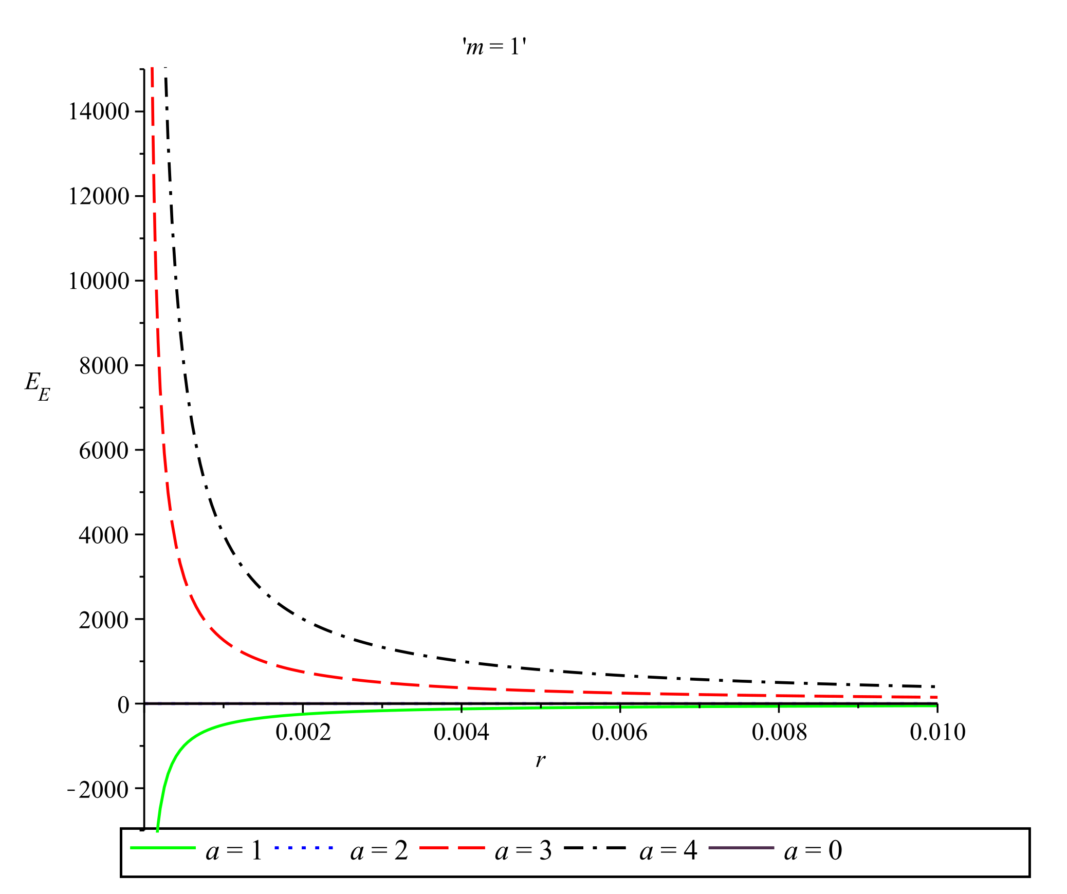
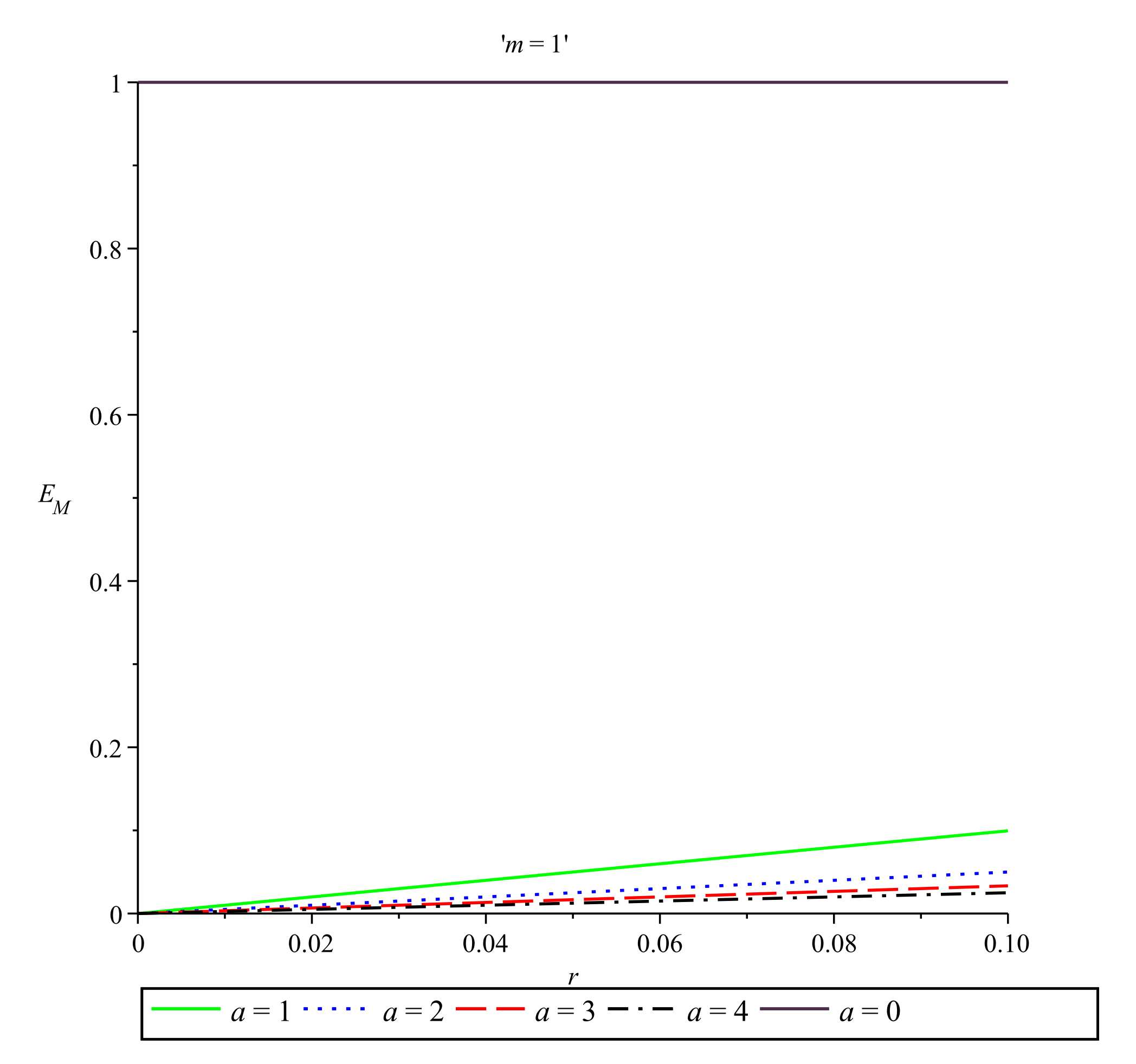
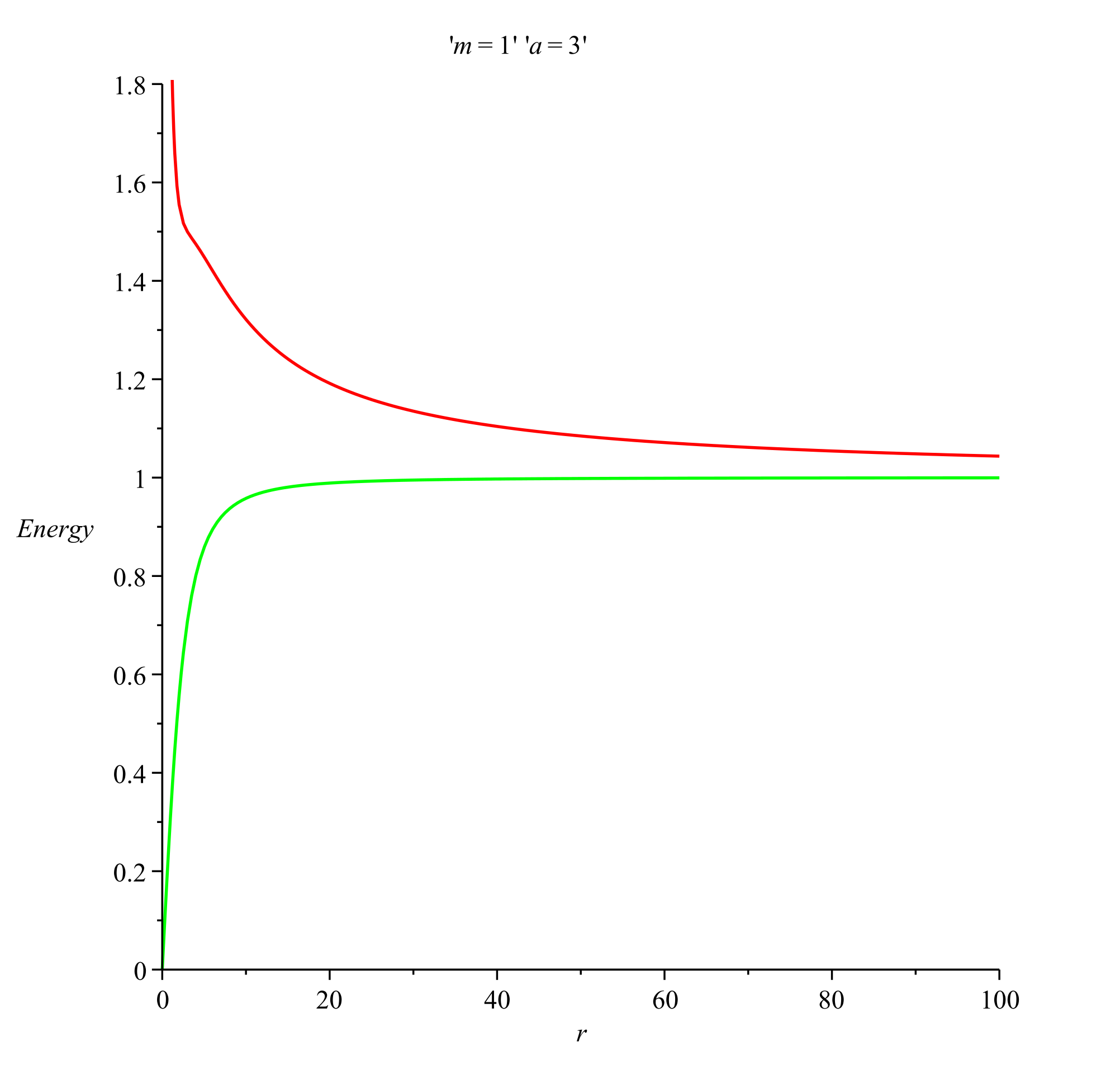
4. Energy-Momentum Distribution of the Simpson–Visser Space-Time

In the case of the Einstein prescription, in order to calculate the energy-momentum the metric given by (1) has to be converted into Schwarzschild Cartesian coordinates using the coordinate transformation $x=rsin\theta cos\varphi ,$$y=rsin\theta sin\varphi ,$$z=rcos\theta$. Then, the metric (1) becomes

$$d{s}^2=B\left(r\right)d{t}^2-(d{x}^2+d{y}^2+d{z}^2)-\frac{A\left(r\right)-1}{r^2}{(xdx+ydy+zdz)}^2.$$

(16)

The components of the superpotential $h_{\mu }^{0i}$ (needed for the calculation of (8)) for $\mu =0,1,2,3$ and $i=1,2,3$ in quasi-Cartesian coordinates vanish

$$\begin{array}{cc}\hfill & h_1^{01}=h_1^{02}=h_1^{03}=0,\hfill \\ \hfill & h_2^{01}=h_2^{02}=h_2^{03}=0,\hfill \\ \hfill & h_3^{01}=h_3^{02}=h_3^{03}=0.\hfill \end{array}$$

(17)

The non-vanishing components of the superpotential have the expressions

$$h_0^{01}=\frac{2x}{r^4}[(1-\frac{2m}{{(r^2+a^2)}^{1/2}})(a^2-r^2)+r^2],$$

(18)

$$h_0^{02}=\frac{2y}{r^4}[(1-\frac{2m}{{(r^2+a^2)}^{1/2}})(a^2-r^2)+r^2],$$

(19)

$$h_0^{03}=\frac{2z}{r^4}[(1-\frac{2m}{{(r^2+a^2)}^{1/2}})(a^2-r^2)+r^2].$$

(20)

Now, using the Equations (8), (16), and (18)–(20), we get for the energy distribution in the Einstein prescription for the Simpson–Visser space-time

$$E_E=\frac{[(1-\frac{2m}{{(r^2+a^2)}^{1/2}})(a^2-r^2)+r^2]}{2r}.$$

(21)

Applying Equations (8) and (17) we obtain that all the momentum components vanish:

$$P_x=P_y=P_z=0.$$

(22)

Figure 1 shows the energy distribution in the Einstein prescription (21) as a function of r for $m=1$ and five different values of the parameter a.

In Figure 2, using the same five values of the parameter a with $m=1$, we have plotted the Einstein energy distribution as a function of r near the origin.

To apply the Møller prescription, the Schwarzschild coordinates $\{t,$$r,$ $\theta ,$$\varphi \}$ have to be used for the line element (1) and the metric function given by (2). After performing the calculations, we find only one non-vanishing component of the Møller superpotential (10), namely

$$M_0^{01}=\frac{2mr}{{(r^2+a^2)}^{1/2}}sin\theta ,$$

(23)

while all the other components vanish.

Combining the expression given by Equation (23) for the Møller superpotential with Equation (15), we find the energy distribution in the Møller prescription:

$$E_M=\frac{mr}{{(r^2+a^2)}^{1/2}}.$$

(24)

The vanishing of the spatial components of the Møller superpotential leads, as it is expected, to the vanishing of all momentum components. So, we have:

$$P_r=P_{\theta }=P_{\varphi }=0.$$

(25)

In Figure 3, we plot the energy distribution in the Møller prescription for $m=1$ and for five different values of the parameter a. Figure 4 exhibits the behavior of the Møller energy near the origin also for $m=1$ and for five different values of the parameter a.

5. Discussion and Concluding Remarks

In this work, we have investigated the energy-momentum distribution for the static Simpson–Visser space-time. In order to study the energy distribution and the momenta we resorted to the use of the Einstein and Møller prescriptions. From the calculations we found zero values for all the momenta in both pseudotensorial prescriptions. Regarding the results obtained for the energy distributions, we found well-defined expressions, a fact highlighting a dependence on the mass m, the positive metric parameter a, and on the radial coordinate r.

In addition, we studied the limiting behavior of the energy distribution for $r\to 0$ and $r\to \infty$, and for the particular case $a=0$ respectively. Both energies acquire the same value being equal to the ADM mass M (ADM mass) for $r\to \infty$ or for $a=0$.

Table 1. Einstein energy $E_E$ and Møller energy $E_M$ for some limiting and particular cases.

Energy	$\mathit{a}=0$	$\mathit{r}\to 0,\mathit{a}>0$	$\mathit{r}\to \mathit{\infty },\mathit{a}>0$
$E_E$	M	$0(a=2m)$	M
$E_M$	M	0	M

shows the physically meaningful results for these limiting and particular cases.

Based on the limiting and particular cases from Table 1 we conclude that the energy in the prescriptions of Einstein and Møller vanishes near the origin $r\to 0$ (the energy in the Einstein prescription vanishes in the case r tends toward zero for $a=2m$), while for either $r\to \infty$ or $a=0$ both energy distributions acquire the same value M which is the ADM mass. This result agrees with the result obtained by Virbhadra for the energy of the Schwarzschild black hole [26].

In Figure 5 we plot the energy distribution in the Einstein prescription in the particular case of the Ellis–Bronnikov wormhole metric for $a\ne 0$ and $m=0$. Indeed, in this case the Einstein energy (21) is not zero, but it is positive and equals $a^2/2r$. Figure 6 presents the behavior of the Einstein energy distribution as a function of r for the same particular case of the Ellis–Bronnikov wormhole metric with $a\ne 0$ and $m=0$ near the origin. Note that in this case the energy (24) in the Møller prescription is equal to zero.

Figure 7 shows the behavior of the Einstein and Møller energy in the case $m=1$ and $a=3$. In Figure 8 we present the Einstein and Moller energy near the origin for $m=1$ and $a=3$. At this point in the discussion we have to emphasize that the behavior of the energy for the Simpson–Visser solution is very interesting and is clearly influenced by the value of the parameter a. For $a=0$ and $m\ne 0$ the Simpson–Visser space-time corresponds to the Schwarzschild metric and the energy in both the Einstein and Møller prescriptions is equal to the ADM mass M, i.e., $E_E=M$ and $E_M=M$, respectively. In the case of the regular black hole metric obtained for $a<2m$, the energy in the Einstein prescription exhibits a small region of negativity beyond which it becomes an increasing positive function of r until it reaches a maximum value. After taking this maximum, the energy decreases to the ADM mass M. For a one-way traversable wormhole metric with a null throat for $a=2m$, the Einstein energy takes only positive values and after increasing and taking a maximum it tends toward the ADM mass M. In the case of a two-way traversable wormhole metric space-time of the Morris–Thorne type for $a>2m$, the energy in the Einstein prescription is everywhere positive and decreases from a maximum value to the ADM mass M. For the energy in the Møller prescription we conclude that for $m\ne 0$ and for any value of the parameter $a>0$ the energy is a positive and increasing function of r and reaches a maximum value which is the ADM mass for r tending toward infinity. In the case $a=0$ and $m\ne 0$, which corresponds to the Schwarzschild metric, the energy in the Møller prescription is equal to the ADM mass M.

The obtained results for the Einstein energy $E_E$ and the Møller energy $E_M$ come to support the use of the Einstein and Møller prescriptions for the evaluation of the energy of a gravitational background, specifying that the positive energy regions can serve as a convergent gravitational lens, while the negative one can serve as a divergent gravitational lens [56]. In fact, the Simpson–Visser metric and its generalizations appear to be extremely advantageous for a deeper understanding of strong-field gravitational lensing of light reflected by a photon sphere of black holes and wormholes [55,57,58,59]. Further, the small region of negativity in the expressions of the Einstein energy $E_E$ in the case $a<2m$ indicates some difficulty in the physically meaningful interpretation of the energy in certain regions of a specific space-time.

As a perspective for future work, the application of other energy-momentum prescriptions and the comparison of the relevant results is planned for the metric considered in the present paper.

References

1. Einstein, A. On the general theory of relativity. In Sitzungsberichte der Königlich Preussischen Akademie der Wissenschaften zu Berlin; Deutsche Akademie der Wissenschaften zu Berlin: Berlin, Germany, 1915; Volume 47, pp. 778–786, Addendum: Volume 47, pp. 799–801; Available online: https://einsteinpapers.press.princeton.edu/vol6-doc/ (accessed on 15 June 2021).
2. Trautman, A. Conservation laws in general relativity. In Gravitation: An Introduction to Current Research; Witten, L., Ed.; John Wiley & Sons: New York, NY, USA, 1962; p. 169. [Google Scholar]
3. Landau, L.D.; Lifshitz, E.M. The Classical Theory of Fields; Pergamon Press: New York, NY, USA, 1987; p. 280. [Google Scholar]
4. Papapetrou, A. Equations of motion in general relativity. Proc. Phys. Soc. A 1951, 64, 57. [Google Scholar] [CrossRef]
5. Bergmann, P.G.; Thomson, R. Spin and angular momentum in general relativity. Phys. Rev. 1953, 89, 400–407. [Google Scholar] [CrossRef]
6. Møller, C. On the localization of the energy of a physical system in the general theory of relativity. Ann. Phys. 1958, 4, 347–371. [Google Scholar] [CrossRef]
7. Weinberg, S. Gravitation and Cosmology: Principles and Applications of General Theory of Relativity; John Wiley & Sons: New York, NY, USA, 1972; p. 165. [Google Scholar]
8. Bergqvist, G. Positivity and definitions of mass. Class. Quantum Gravity 1992, 9, 1917. [Google Scholar] [CrossRef]
9. Chen, C.-M.; Nester, J.M. Quasi local quantities for general relativity and other gravity theories. Class. Quantum Gravity 1999, 16, 1279. [Google Scholar] [CrossRef] [Green Version]
10. Sinha, A.K.; Pandey, G.K.; Bhaskar, A.K.; Rai, B.C.; Jha, A.K.; Kumar, S.; Xulu, S.S. Effective gravitational mass of the Ayón-Beato and García metric. Mod. Phys. Lett. 2015, 30, 1550120. [Google Scholar] [CrossRef] [Green Version]
11. Tripathy, S.K.; Mishra, B.; Pandey, G.K.; Singh, A.K.; Kumar, T.; Xulu, S.S. Energy and momentum of Bianchi type VIh universes. Adv. High Energy Phys. 2015, 2015, 705262. [Google Scholar] [CrossRef] [Green Version]
12. Saleh, M.; Thomas, B.B.; Kofane, T.C. Energy distribution and thermodynamics of the quantum-corrected Schwarzschild black hole. Chin. Phys. Lett. 2017, 34, 080401. [Google Scholar] [CrossRef] [Green Version]
13. Sahoo, P.K.; Mahanta, K.L.; Goit, D.; Sinha, A.K.; Xulu, S.S.; Das, U.R.; Prasad, A.; Prasad, R. Einstein energy-momentum complex for a phantom black hole metric. Chin. Phys. Lett. 2015, 32, 020402. [Google Scholar] [CrossRef] [Green Version]
14. Yang, I.-C. Some characters of the energy distribution for a charged wormhole. Chin. J. Phys. 2015, 53, 110108-1–110108-4. [Google Scholar]
15. Radinschi, I.; Rahaman, F.; Ghosh, A. On the energy of charged black holes in generalized dilaton-axion gravity. Int. J. Theor. Phys. 2010, 49, 943–956. [Google Scholar] [CrossRef] [Green Version]
16. Yang, I.-C.; Lin, C.-L.; Radinschi, I. The energy of a regular black hole in general relativity coupled to nonlinear electrodynamics. Int. J. Theor. Phys. 2009, 48, 248–255. [Google Scholar] [CrossRef] [Green Version]
17. Vagenas, E.C. Energy distribution in 2d stringy black hole backgrounds. Int. J. Mod. Phys. 2003, 18, 5781–5794. [Google Scholar] [CrossRef] [Green Version]
18. Radinschi, I.; Rahaman, F.; Banerjee, A. On the energy of Hořava-Lifshitz black holes. Int. J. Theor. Phys. 2011, 50, 2906–2916. [Google Scholar] [CrossRef]
19. Radinschi, I.; Rahaman, F.; Grammenos, T.; Islam, S. Einstein and Møller energy-momentum complexes for a new regular black hole solution with a nonlinear electrodynamics source. Adv. High Energy Phys. 2016, 2016, 9049308. [Google Scholar] [CrossRef]
20. Radinschi, I.; Grammenos, T.; Rahaman, F.; Spanou, A.; Islam, S.; Chattopadhyay, S.; Pasqua, A. Energy-momentum for a charged nonsingular black hole solution with a nonlinear mass function. Adv. High Energy Phys. 2017, 2017, 7656389. [Google Scholar] [CrossRef]
21. Abdel-Megied, M.; Gad, R.M. Møller’s Energy in the Kantowski-Sachs Space-Time. Adv. High Energy Phys. 2010, 2010, 379473. [Google Scholar] [CrossRef] [Green Version]
22. Radinschi, I.; Grammenos, T.; Rahaman, F.; Cazacu, M.M.; Spanou, A.; Chakraborty, J. On the energy of a non-singular black hole solution satisfying the weak energy condition. Universe 2020, 6, 169. [Google Scholar] [CrossRef]
23. Balart, L. Energy distribution of (2+1)-dimensional black holes with nonlinear electrodynamics. Mod. Phys. Lett. A 2009, 24, 2777–2785. [Google Scholar] [CrossRef]
24. Matyjasek, J. Some remarks on the Einstein and Møller pseudotensors for static and spherically-symmetric configurations. Mod. Phys. Lett. A 2008, 23, 591–601. [Google Scholar] [CrossRef] [Green Version]
25. Aguirregabiria, J.M.; Chamorro, A.; Virbhadra, K.S. Energy and angular momentum of charged rotating black holes. Gen. Relativ. Gravit. 1996, 28, 1393–1400. [Google Scholar] [CrossRef] [Green Version]
26. Virbhadra, K.S. Naked singularities and Seifert’s conjecture. Phys. Rev. D 1999, 60, 104041. [Google Scholar] [CrossRef] [Green Version]
27. Xulu, S.S. Bergmann–Thomson energy-momentum complex for solutions more general than the Kerr-Schild class. Int. J. Theor. Phys. 2007, 46, 2915–2922. [Google Scholar] [CrossRef] [Green Version]
28. Grammenos, T.; Radinschi, I. Energy distribution in a Schwarzschild-like spacetime. Int. J. Theor. Phys. 2007, 46, 1055–1064. [Google Scholar] [CrossRef] [Green Version]
29. Vagenas, E.C. Energy distribution in the dyadosphere of a Reissner-Nordström black hole in Møller’s prescription. Mod. Phys. Lett. A 2006, 21, 1947–1956. [Google Scholar] [CrossRef] [Green Version]
30. Bel, L. Définition d’une densité d’énergie et d’un état de radiation totale généralisée. Comptes Rendus Del’Acad. Sci. 1958, 246, 3015–3018. [Google Scholar]
31. Bonilla, M.A.G.; Senovilla, J.M.M. Some properties of the Bel and Bel-Robinson tensors. Gen. Relativ. Gravit. 1997, 29, 91–116. [Google Scholar] [CrossRef]
32. Senovilla, J.M. Super-energy tensors. Class. Quantum Gravity 2000, 17, 2799–2841. [Google Scholar] [CrossRef] [Green Version]
33. Penrose, R. Quasi-local mass and angular momentum in general relativity. Proc. R. Soc. Lond. A Math. Phys. Eng. Sci. 1982, 381, 53–63. [Google Scholar]
34. Tod, K.P. Some examples of Penrose’s quasilocal mass construction. Proc. R. Soc. Lond. A Math. Phys. Eng. Sci. 1983, 388, 457–477. [Google Scholar]
35. Brown, J.D.; York, J.W. Quasilocal energy and conserved charges derived from the gravitational action. Phys. Rev. D 1993, 47, 1407. [Google Scholar] [CrossRef] [Green Version]
36. Hayward, S.A. Quasilocal gravitational energy. Phys. Rev. D 1994, 49, 831–839. [Google Scholar] [CrossRef] [PubMed] [Green Version]
37. Chen, C.-M.; Liu, J.-L.; Nester, J.M. Gravitational energy is well defined. Int. J. Mod. Phys. D 2018, 27, 1847017. [Google Scholar] [CrossRef]
38. Chen, C.-M.; Liu, J.-L.; Nester, J.M. Quasi-local energy from a Minkowski reference. Gen. Relativ. Gravit. 2018, 50, 158. [Google Scholar] [CrossRef] [Green Version]
39. Møller, C. The four-momentum of an insular system in general relativity. Nucl. Phys. 1964, 57, 330–338. [Google Scholar] [CrossRef]
40. Hayashi, K.; Shirafuji, T. New general relativity. Phys. Rev. D 1979, 19, 3524. [Google Scholar] [CrossRef]
41. Maluf, J.W.; Veiga, M.V.O.; da Rocha-Neto, J.F. Regularized expression for the gravitational energy-momentum in teleparallel gravity and the principle of equivalence. Class. Quantum Gravity 2007, 39, 227–240. [Google Scholar] [CrossRef] [Green Version]
42. Nester, J.M.; So, L.L.; Vargas, T. Energy of homogeneous cosmologies. Phys. Rev. D 2008, 78, 044035. [Google Scholar] [CrossRef] [Green Version]
43. Nashed, G.G.L. Energy of spherically symmetric space-times on regularizing teleparallelism. Int. J. Mod. Phys. A 2010, 25, 28–83. [Google Scholar] [CrossRef] [Green Version]
44. Sousa, A.; Pereira, R.B.; Silva, A.C. Energy and angular momentum densities in a Gödel-type universe in teleparallel geometry. Gravit. Cosmol. 2010, 16, 25–33. [Google Scholar] [CrossRef]
45. Sharif, M.; Jawad, A. Energy contents of some well-known solutions in teleparallel gravity. Astrophys. Space Sci. 2011, 331, 257–263. [Google Scholar] [CrossRef] [Green Version]
46. Aygun, S.; Baysal, H.; Aktaş, C.; Yılmaz, I.; Sahoo, P.K.; Tarhan, I.S. Teleparallel energy-momentum distribution of various black hole and wormhole metrics. Int. J. Mod. Phys. A 2018, 33, 1850184. [Google Scholar] [CrossRef]
47. Ganiou, M.G.; Houndjo, M.J.S.; Tossa, J. f (T) gravity and energy distribution in Landau–Lifshitz prescription. Int. J. Mod. Phys. D 2018, 27, 1850039. [Google Scholar] [CrossRef] [Green Version]
48. Simpson, A.; Visser, M. Black-bounce to traversable wormhole. J. Cosmol. Astropart. Phys. 2019, 2, 42. [Google Scholar] [CrossRef] [Green Version]
49. Simpson, A.; Martin-Moruno, P.; Visser, M. Vaidya spacetimes, black-bounces, and traversable wormholes. Class. Quantum Gravity 2019, 36, 145007. [Google Scholar] [CrossRef] [Green Version]
50. Lobo, F.S.N.; Rodrigues, M.E.; Silva, M.V.d.; Simpson, A.; Visser, M. Novel black-bounce spacetimes: Wormholes, regularity, energy conditions, and causal structure. Phys. Rev. D 2021, 103, 0840521. [Google Scholar] [CrossRef]
51. Wheeler, J.A. Geometrodynamics; Academic Press: Cambridge, MA, USA, 1962. [Google Scholar]
52. Izmailov, R.N.; Zhdanov, E.R.; Bhattacharya, A.; Potapov, A.A.; Nandi, K.K. Can massless wormholes mimic a Schwarzschild black hole in the strong field lensing? Eur. Phys. J. Plus 2019, 134, 384. [Google Scholar] [CrossRef]
53. Yusupova, R.M.; Karimov, R.K.; Izmailov, R.N.; Nandi, K.K. Accretion Flow onto Ellis–Bronnikov Wormhole. Universe 2021, 7, 177. [Google Scholar] [CrossRef]
54. Mazza, J.; Franzin, E.; Liberati, S. A novel family of rotating black hole mimickers. J. Cosmol. Astropart. Phys. 2021, 4, 82. [Google Scholar] [CrossRef]
55. Islam, S.U.; Kumar, J.; Ghosh, S.G. Strong gravitational lensing by rotating Simpson–Visser black holes. arXiv 2021, arXiv:2104.00696. [Google Scholar]
56. Virbhadra, K.S.; Ellis, G.F.R. Schwarzschild black hole lensing. Phys. Rev. D 2000, 62, 084003. [Google Scholar] [CrossRef] [Green Version]
57. Tsukamoto, N. Gravitational lensing in the Simpson–Visser black-bounce spacetime in a strong deflection limit. Phys. Rev. D 2021, 103, 024033. [Google Scholar] [CrossRef]
58. Jafarzade, K.; Zangeneh, M.K.; Lobo, F.S.N. Observational optical constraints of the Simpson–Visser black-bounce geometry. arXiv 2021, arXiv:2106.13893. [Google Scholar]
59. Nascimento, J.R.; Petrov, A.Y.; Porfírio, P.J.; Soares, A.R. Gravitational lensing in black-bounce spacetimes. Phys. Rev. D 2020, 102, 044021. [Google Scholar] [CrossRef]
Figure 1. Einstein energy vs. r for m = 1 and a = 0 , a = 1 , a = 2 , a = 3 and a = 4 .
Symmetry 13 01622 g001
Figure 2. Einstein energy near the origin vs. r for m = 1 and a = 0 , a = 1 , a = 2 , a = 3 and a = 4 . The corresponding values on the energy axis for a = 0 and a = 2 are less than the energy values corresponding to a = 1 , a = 3 and a = 4 and are therefore not distinguishable from the x-axis.
Symmetry 13 01622 g002
Figure 3. Møller energy vs. r for m = 1 and a = 0 , a = 1 , a = 2 , a = 3 and a = 4 .
Symmetry 13 01622 g003
Figure 4. Møller energy near the origin vs. r for m = 1 and a = 0 , a = 1 , a = 2 , a = 3 and a = 4 .
Symmetry 13 01622 g004
Figure 5. Einstein energy vs. r for m = 0 and a = 1 , a = 2 , a = 3 and a = 4 .
Symmetry 13 01622 g005
Figure 6. Einstein energy near the origin vs. r for m = 0 and a = 1 , a = 2 , a = 3 and a = 4 .
Symmetry 13 01622 g006
Figure 7. Einstein (red) and Møller (green) energy vs. r for m = 1 and a = 3 .
Symmetry 13 01622 g007
Figure 8. Einstein (red) and Møller (green) energy near the origin vs. r for m = 1 and a = 3 .
Symmetry 13 01622 g008