Article

Identifying Influential Nodes in Complex Networks Based on Node Itself and Neighbor Layer Information

College of Electronic Engineering, National University of Defense Technology, Hefei 230037, China
*
Author to whom correspondence should be addressed.
Symmetry 2021, 13(9), 1570; https://doi.org/10.3390/sym13091570
Submission received: 9 August 2021 / Revised: 15 August 2021 / Accepted: 16 August 2021 / Published: 26 August 2021

Abstract

:
Identifying influential nodes in complex networks is of great significance for clearly understanding network structure and maintaining network stability. Researchers have proposed many classical methods to evaluate the propagation impact of nodes, but there is still some room for improvement in the identification accuracy. Degree centrality is widely used because of its simplicity and convenience, but it has certain limitations. We divide the nodes into neighbor layers according to the distance between the surrounding nodes and the measured node. Considering that the node’s neighbor layer information directly affects the identification result, we propose a new node influence identification method by combining degree centrality information about itself and neighbor layer nodes. This method first superimposes the degree centrality of the node itself with neighbor layer nodes to quantify the effect of neighbor nodes, and then takes the nearest neighborhood several times to characterize node influence. In order to evaluate the efficiency of the proposed method, the susceptible–infected–recovered (SIR) model was used to simulate the propagation process of nodes on multiple real networks. These networks are unweighted and undirected networks, and the adjacency matrix of these networks is symmetric. Comparing the calculation results of each method with the results obtained by SIR model, the experimental results show that the proposed method is more effective in determining the node influence than seven other identification methods.

1. Introduction

The research direction of node influence in complex networks has attracted wide attention in recent years. The main research focus is to rank the influence of nodes to evaluate their importance. In fact, many systems in real life can be considered as complex network systems [1], such as animal networks [2], traffic networks [3], social networks [4], and economic networks. For example, identifying critical nodes in social networks and monitoring them can prevent the mass spread of infectious diseases. Identifying effective drug targets in cellular network systems allows for faster drug action in the body [5]. Numerous studies [6,7,8,9,10,11,12,13] have shown the significant theoretical and practical importance of identifying influential nodes that have a role in network structure and function. In the network, there are often a small number of nodes that support the entire network architecture, and the accurate identification of these nodes helps to maintain the stability of the network and ensure the normal operation of network functions.
Currently, researchers have proposed many classical methods for identifying influential nodes, including degree centrality [6], betweenness centrality [7], closeness centrality [8], eigenvector centrality [9], bridging centrality [10], LeaderRank [11], k-shell decomposition [12], and H-index [13]. Among these methods, the most widely used are degree centrality and k-shell decomposition. Degree centrality is simpler and more intuitive because it can be expressed directly in terms of the number of connected nodes, and it can be easily applied to large-scale networks. However, degree centrality and k-shell decomposition also have certain limitations. Degree centrality considers the most local information of nodes, while k-shell decomposition divides many nodes into the same layer; both easily cause the node sorting to be too coarse-grained. Researchers have made many efforts to improve the problem of coarse-graining. Joonhyun et al. [14] proposed an improved coreness method that introduces information on neighborhoods to define node influence. Ahmed et al. [15] proposed a method to identify the influence of nodes according to the circular area density formula by taking the nodes’ own degree centrality and the shortest path distance between two nodes as mass and radius, respectively. Li et al. [16] used the gravity model to propose a method that uses neighborhood information and path information to measure the influence of nodes in the spreading process. Li et al. [17] considered the role of the clustering coefficient, and they combined the clustering coefficient and the sum of the degree centrality of the nearest neighbor node to quantify node influence. Sheng et al. [18] combined the global and local structural characteristics of the network, global information reflecting the proximity to other nodes in the network, and local information as the contribution value of the nearest neighbor node to the measured node. Yang et al. [19] first proposed an improved k-shell decomposition method based on the k-shell value and the number of iterations of node removal in the k-shell decomposition, and then combined the improved method with degree centrality and the shortest path length to characterize the node influence. Zareie et al. [20] proposed an improved clustering ranking approach, which takes the common hierarchical structure of nodes and their neighborhood set into account. Yan et al. [21] propose, a new method that considers the local topological characteristics of nodes, center position of nodes, and effect of neighbor nodes.
The above methods are from different perspectives to solve the problem of insufficient differentiation in the process of node identification, but there is still room for improvement in recognition accuracy. In order to improve the accuracy of identification, we propose a new method of identifying node influence by combining information on the node itself and neighbor layers, which first superimposes the degree centrality of the node itself and neighborhood nodes within a certain range, and then considers the contribution of multiple fetches of nearest neighbor information to the accuracy of the results. To verify the effectiveness of the proposed method, this paper uses the SIR model [22,23] to perform 1000 independent simulations on multiple real networks to obtain the information dissemination ability of nodes. The proposed method in this paper is compared with degree centrality, betweenness centrality, closeness centrality, area density centrality [15], GM method [16], CLD method [17], and GLI method [19] in terms of discrimination and accuracy. The experimental results show that the proposed method in this paper can distinguish the influence among nodes and improve the recognition accuracy.
This section clarified the background of the study and the current research progress in the field. The rest of the paper is framed as follows: Section 2 explains the definition of comparison methods and the detailed idea of the proposed method based on information on the node itself and neighbor layers. The datasets used in this paper and the evaluation criteria for the experiments are given in Section 3. In Section 4, we present verification experiments in terms of the discrimination and accuracy comparing the proposed method with others. The final summary of this paper is given in Section 5.

2. Materials and Methods

An unweighted and undirected network is represented by G = (V, E), where V = {v1, v2, …, vn} represents the set of n nodes, and E = {e1, e2, …, em} represents the set of m edges. We can use adjacency matrix A = (aij)n × n to represent the structural characteristics of a complex network, where the adjacency matrix is symmetric. The element aij in the matrix can represent the edge information between any two nodes. If aij = 1, it means that there is a connection relationship between two nodes; otherwise, there is no connection relationship. Hereafter, ki represents the degree centrality of node i.

2.1. Node Influence Based on Node and Neighbor Layer Information

Degree centrality represents the most local information of nodes in the network. It only reflects the importance of nodes according to the nodes themselves and ignores the influence of the surrounding nodes. Numerous studies have shown that the neighbor layer information of a node has an indispensable effect on node influence. During the spreading process, the node will certainly spread information to neighbor nodes through their connection in sequence until it cannot be transmitted. It is destined that the surrounding environment of the node will directly affect the spreading ability of the node. In order to explore the role of neighbor layer information on node spreading, this paper proposes a node influence identification method based on the node itself and neighbor layer information, called the NINL method. The main idea of this method is to consider the local information within a certain range of nodes. First, a radius is defined according to the average path length of the network, and the main consideration is the influence of the surrounding environment caused by the set of nodes within this radius. Then, the information of the nodes themselves is combined with the information of nodes within this range, and the initial local information is defined as
N I N L 0 i = k i + j k j , j Γ i L ,
where Γ is used to represent nodes within a certain distance from node i, L refers to the average path length of the network, and ⌈x⌉ refers to the smallest integer not smaller than x. To reflect the influence of nearest neighbor information more comprehensively, Equation (1) is extended to define the influence of nodes by using recursion, and the recursive formula is shown below.
N I N L 1 i = j Γ i N I N L 0 j N I N L 2 i = j Γ i N I N L 1 j , N I N L p i = j Γ i N I N L p 1 j
where p refers to the number of iterations, and Γ i represents the nearest neighborhood nodes of node i. We can speculate the p-value according to some networks. In this paper, we chose p = 3, for reasons discussed in the next section. We use an example network below to illustrate the calculation process in detail.
Taking the example network of 13 nodes in Figure 1, the average path length of the network is calculated as L = sum(dij)/(n × (n−1)) = 358/(13 × (13−1)) ≈ 2.2949. Thus, we can get ⌈L⌉ = 3. The following takes node 1 as an example to g ive the calculation process of NINL0(1). First, we need to calculate degree centrality of each node, as shown below.
k1 = 1, k2 = 1, k3 = 4, k4 = 6, k5 = 4, k6 = 3, k7 = 1, k8 = 4, k9 = 5, k10 = 2, k11 = 2, k12 = 4, k13 = 1.
Then, according to ceil(L) = 3, we can get that the first-level neighbor node set of node 1 is {3}, the second-level neighbor node set is {4, 5, 6}, and the third-level neighbor node set is {2, 7, 8, 9}. To sum up, the set of neighbor nodes within the three layers is {2, 3, 4, 5, 6, 7, 8, 9}; thus, NINL0(1) = k1 + (k2 + k3+ k4 + k5 + k6 + k7 + k8 + k9) = 1 + (1 + 4 + 6 + 4 + 3 + 1 + 4 + 5) = 1 + 28 = 29. Table 1 shows the calculation results of the node influence of NINL0NINL3 of the example network.
From the table, we can see that NINL0 defines nodes 2, 3, 5, 6, 7, 10, 11, and 12 as the same value, and nodes 4, 8, and 9 as the same value. After getting the nearest neighbor node information for the first time, NINL1 defines nodes 1 and 13 as the same value, nodes 2 and 7 as the same value, nodes 5 and 8 as the same value, and nodes 10 and 11 as the same value. NINL2 also distinguishes the influence of nodes 1 and 13. The influence of nodes 5 and 8 was also identified. As for nodes 2 and 7, they could not be distinguished because they had the same information about themselves and their neighbors as nodes 10 and 11. At the same time, we can observe that nodes 2 and 7 were locally symmetrical, just like nodes 10 and 11. The above phenomenon shows that the proposed NINL method can effectively distinguish the influence of the nodes in the sample network.
The specific computational flow of Algorithm 1 is shown below.
Algorithm 1. The NINLp Method
Input: the network G = (V, E)
Output: node influence of NINLp centrality
1: for i = 1 to |V|
2:   for j = 1 to |V|
3:     calculate the shortest path length between node i and node j
4:   end for
5: end for
6: calculate average path length L
7: for i = 1 to |V|
8:   calculate the Degree centrality of node i
9: end for
10: for i = 1 to |V|
11:   find the neighbor nodes with a radius of ceil(L) from the node i
12:   calculate NINL0 of node i according to Equation (1)
13: end for
14: for i = 1 to |V|
15:   find the nearest neighbor nodes of node i
16: end for
17: set the value of p
18: Recursively calculate NINLp centrality according to Equation (2)
19: return NINLp centrality

2.2. Benchmark Methods

2.2.1. Degree Centrality

Degree centrality [6] in complex network reflects the node’s connection information, which can be expressed by the number of nearest neighbor nodes. A greater value of the degree denotes a greater influence of the node. The degree centrality of node i can be defined as
k i = j = 1 n a i j .
In addition, degree centrality can be normalized to
D C i = k i n 1 .

2.2.2. Betweenness Centrality

Betweenness centrality [7] refers to the ratio of the number of shortest paths through a node to the number of shortest paths for all pairs of nodes in the network. The betweenness centrality of node i can be expressed as
B C ( i ) = s t i V g s t i g s t ,
where g s t i represents the number of shortest paths through node i, and g s t refers to the number of shortest paths for all node pairs in the node set.

2.2.3. Closeness Centrality

Closeness centrality [8] refers to the reciprocal of the sum of the shortest path lengths between a node and other nodes. This method takes the global information of the network into account. The formula is as follows:
C C i = n 1 j i V d i j ,
where dij refers to the shortest path length between node i and node j.

2.2.4. Density Centrality

The principle of density centrality [15] is the circular area density formula. The degree centrality of the node and the path length between two nodes are used as the mass and radius in the density formula, which highlights the influence of the number of neighbor nodes. The density centrality of node i can be defined as
D N C i = j Γ i r k i π d i j 2 ,
where Γ i r refers to the set of nodes whose path length is less than or equal to r; r = 3 was applied in the original paper.

2.2.5. Gravity Model

The gravity model [16] is derived from the law of gravity. It considers the relationship between node neighbor layer information and path length. The degree centrality is regarded as quality, and the shortest path length is taken as the distance. The influence of node i is expressed as
G M ( i ) = j i k i k j d i j 2 .

2.2.6. Clustered Local-Degree (CLD) Method

The clustered local-degree method [17] first obtains the sum of degree centrality of the nearest neighbor nodes, and then links the obtained results with the clustering coefficient of the nodes to propose a method for identifying the influence of nodes, as expressed below.
C L D i = ( 1 + C i ) j Γ i k j ,
where Ci represents clustering coefficient of node i, and Γ i represents the nearest neighborhood.

2.2.7. GLI Method

The GLI method [19] contains both global location information and local structure information. First, considering that the k-shell decomposition method divides many nodes into the same layer, an improved k-shell decomposition method (Iks) was defined as follows:
I k s i = k s i + n i t ( i ) ,
where ks(i) refers to the level of node i after k-shell decomposition, and nit(i) refers to the number of iterations when the node is deleted during the iteration. Then, researchers proposed a new node influence identification method named the GLI method by linking the obtained improved method with degree centrality and path information, expressed as follows:
G L I i = exp I k s i + k i i = 1 n I k s i + k i × j Γ i r I k s j + k j d i j .
In this case, the neighbors within three hops of the node are considered, i.e., r = 3.

3. Experimental Data and Evaluation Criteria

3.1. Datasets

In order to verify the effectiveness of the method proposed in this paper, several real networks with different structures were selected for experiments. The real networks used in this article were the Contiguous network [24], Dolphin network [25], Polbooks network [26], Word network [27], Jazz network [28], Slavko Facebook network [26], USAir network [29], Netscience network [27], Infectious network [30], and Email network [31]. The datasets can also be found at https://github.com/Ismileo/Datasets, accessed on 19 July 2021 [32]. Table 2 shows the basic topological properties of the networks. In the table, n and m denote the number of nodes in the network and the number of connected edges, respectively. kmax refers to the maximum degree, <k> refers to the average degree of all network nodes, D is the network diameter, L is the average path length, C refers to the average clustering coefficient, and r refers to the assortative coefficient of the network [33].

3.2. Spreading Model and Evaluation Criteria

3.2.1. SIR Model

The SIR model can be used to describe the process of information dissemination, which is widely used in the field of infectious diseases. In this paper, the SIR model was used to simulate the node infection process to obtain the influence of nodes. Nodes in the SIR spreading model can exist in the following three states: (i) susceptible (S), (ii) infected (I), and (iii) recovered (R). The susceptible state means that the node is not currently infected but has the possibility of being infected, the infected state means that it has been infected and can infect other nodes with a certain probability, and the recovered state means that it cannot infect other nodes and cannot be infected by other nodes. The specific process is to first set a node to be in an infected state and other nodes to be in a susceptible state, and then the infected node can infect the susceptible nodes with a certain spread probability β, while the infected nodes will also be converted to the recovery state with a recovery probability λ = 1, until the whole process is in a stable state. In this paper, the spreading probability β was set to take a value around the spreading threshold [34], and the total number of nodes infected by a node during spreading was considered as the influence of a node. In this article, we carried out 1000 independent simulations, and the average value was used to represent the node influence according to SIR model. The proposed method and other methods were compared on the basis of the ranking results obtained from the SIR spreading model. A closer ranking result to the SIR model denotes a higher accuracy.

3.2.2. CCDF Method

In the process of obtaining node influence, there will be multiple nodes with the same value. The complementary cumulative distribution function (CCDF) can show the probability distribution of the sorting results, and the effect of each method can be observed through the change trend. The specific formula is as follows:
C C D F ( r ) = 1 i = 1 r n i n ,
where ni refers to the numerical value in the i-th place in a ranking list, and n refers the number of all nodes. When the number of different values in a ranking list is closer to n, it means that the method can distinguish the influence of each node more effectively, and the decrease rate of CCDF will be smaller.

3.2.3. Kendall Correlation Coefficient

The Kendall correlation coefficient [35] is usually used to evaluate the correlation of two sorting results, with a value range of [−1,1]; when the value is 1, it means that the two groups have the same sorting result, whereas a value of −1 means that two sets of numbers are completely negatively correlated, and a value of 0 means the sorting results are independent of each other. Suppose there exist two sequences X and Y with n elements, whereby the sequence XYi = (xi, yi) is formed by taking the elements at the same position in the sequences X and Y. For any two elements XYi and XYj in the newly composed sequence, there are three cases: (i) if xi > xj and yi > yj or xi < xj and yi < yj, it is said that the node pairs are concordant; (ii) if xi > xj and yi < yj or xi < xj and yi > yj, the node pairs are discordant; (iii) if the above conditions are not met, the node pairs are neither concordant nor discordant. The Kendall correlation coefficient can be expressed by the following formula:
τ X , Y = 2 C D n n 1 ,
where C refers to the number of concordant pairs, and D is the number of discordant pairs. It is worth noting that, in addition to the Kendall correlation coefficient, there are the Pearson correlation coefficient, Spearman’s rank correlation coefficient, and Gamma correlation coefficient [36].

3.2.4. Jaccard Similarity Coefficient

Jaccard similarity [37] can be used to evaluate the similarity of the two methods in the sorting results, expressed as the ratio of the number of intersection nodes to the number of union nodes. The specific formula is
J r X , Y = X r Y r X r Y r ,
where X(r) and Y(r) refer to the first r elements in the two lists X and Y, respectively. A closer Jr result to 1 denotes that the two lists are closer, which can be used to evaluate the accuracy of a certain ratio of node identification.

4. Experiment and Analysis

In this section, the CCDF, Kendall correlation coefficient, influence consistency, and Jaccard similarity coefficient were used to evaluate the proposed method. The experimental process and results are presented below.

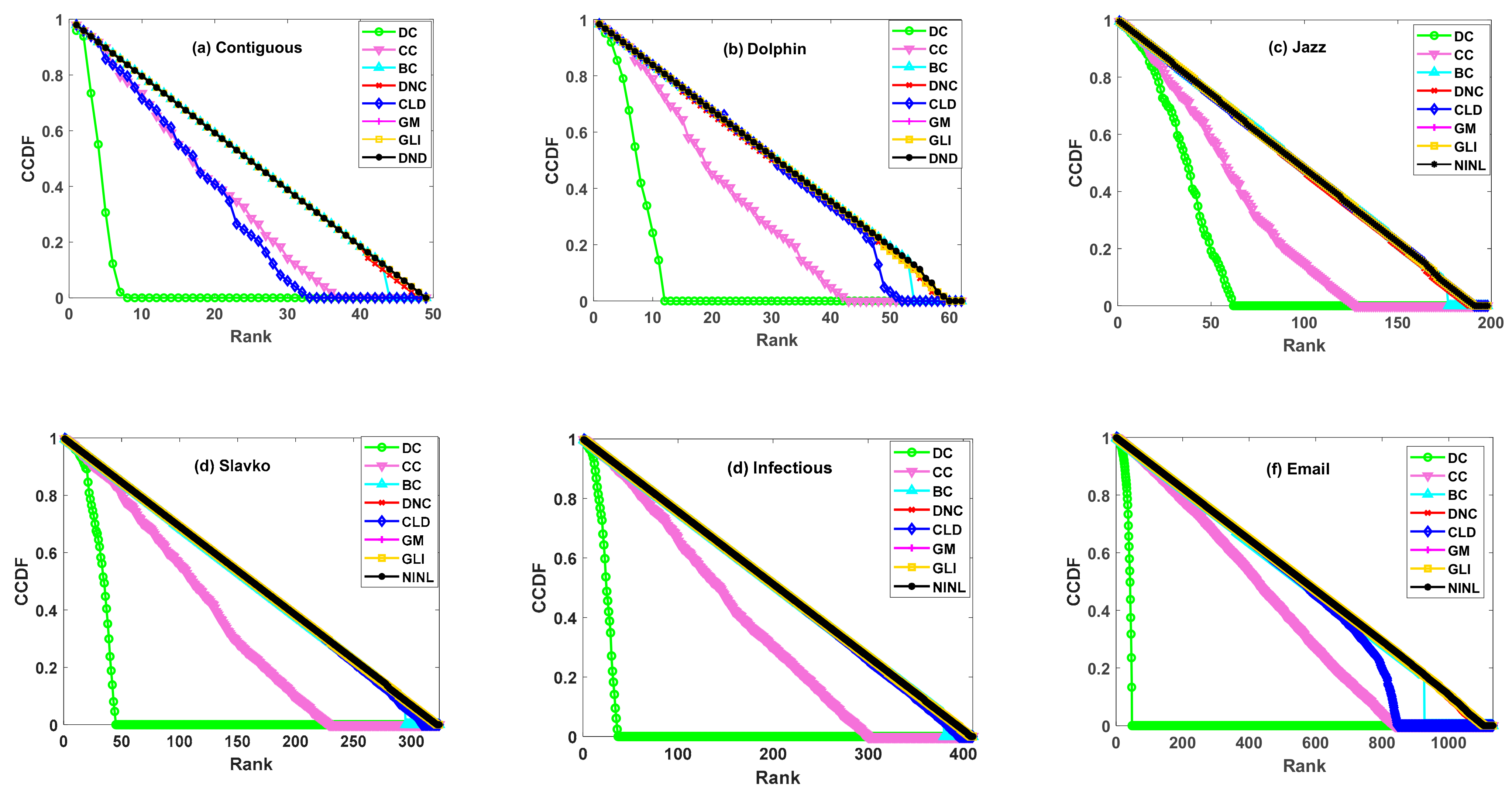
4.1. Discrimination Experiment

The easy accessibility of degree centrality has led to it being widely used. Degree centrality can be expressed only by the number of nearest neighbor nodes. This is its advantage and its disadvantage. The disadvantage is that it is too simple to represent node information using degree centrality, which will cause multiple nodes to be defined with the same influence. The information of the nodes is also influenced by the environmental elements, which leads to the majority of nodes having different influence results. Therefore, the first step of an effective method should be able to distinguish the importance of each node. Only by distinguishing the influence of each node can an effective ranking be carried out. To verify the discernibility of each method on the node, this paper used the CCDF method to determine the discrimination effect of the obtained sorting results, as shown in Figure 2.
Figure 2 shows the change trend of CCDF obtained using each method on the six networks of Contiguous, Dolphin, Jazz, Slavko, Infectious, and Email. The downward trend of CCDF at a certain point is determined by the frequency of the corresponding ranking point. If the number of corresponding ranking nodes is higher, the change trend is more drastic. The closer the CCDF is to a straight line, the better the effect is of distinguishing node influence. From the results in Figure 2, we can see that DC and CC methods declined faster among the six networks compared to other methods. DC represents the most local information of nodes; hence, it is very easy to define multiple nodes as the same value, which also highlights the biggest shortcoming of the DC method. Furthermore, CC considers the global shortest path length, and the result of superposition is likely to have the same value. The CLD method has a certain limitation because it only considers the node’s own clustering coefficient and the degree centrality of the nearest neighbor nodes, which results in it not being able to distinguish the influence of nodes well. It can also be observed that the BC method can make an effective distinction at an early stage, but there is a sudden decrease at a later stage. The BC method considers the pivotal role of nodes in the network, but there are also several nodes with insignificant pivotal roles in the network. Such nodes will also vary in importance when they are affected by the environment; however, the BC method cannot distinguish this phenomenon. Overall, GM, GLI, and the method proposed in this paper best discriminated the influence of network nodes, basically demonstrating a straight line. It can be concluded that the method proposed in this paper can successfully distinguish the spreading influence of each node.

4.2. Accuracy Experiment

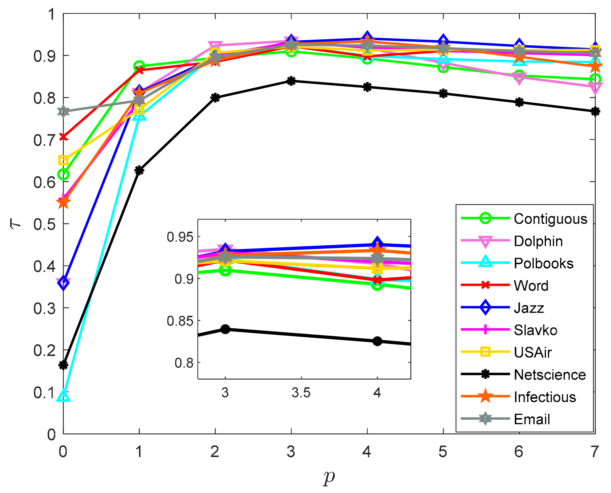
4.2.1. Selection of p-Value

In order to ensure the rationality of the value of p, this paper used the Kendall coefficient to carry out simulation research on 10 networks, and the simulation results are shown in Figure 3. We set the value of p as the x-axis and Kendall coefficient as the y-axis. To observe the changes more clearly, a partially enlarged subfigure is presented. According to the experimental results, the Kendall coefficient value increased with the increase in p at the beginning, but stopped increasing after reaching a threshold. In the partial enlarged image, we can see that the Kendall values of the networks except for Jazz and Infectious began to decrease after a p-value of 3, whereas the Jazz and Infectious networks began to decrease after a p-value of 4. Therefore, this paper selected p = 3 for subsequent experiments.
Table 3 shows the Kendall values obtained by comparing all methods and the SIR model using the 10 networks. In this paper, the spreading probability β set in the SIR model was the value near the spreading threshold βth, and 1000 independent SIR model simulation experiments were conducted to represent the influence of a node with the average value. According to the experimental results in Table 3, the BC method had the worst effect in identifying nodes. Comparing the Kendall coefficients of the CLD and DC methods, it can be found that superimposing the information of the nearest neighbor nodes could improve the accuracy of node identification. Comparing the GM, GLI, and DC methods, it can be found that the combination of the node itself and the neighbor layer information could more effectively identify influential nodes. From this table, we can see that the NINL method proposed in this paper had a more obvious recognition effect and a more accurate effect compared with other methods, thus verifying that accumulating the nearest neighbor information several times after combining node and neighbor layer information can more accurately reflect the node influence and achieve effective identification.

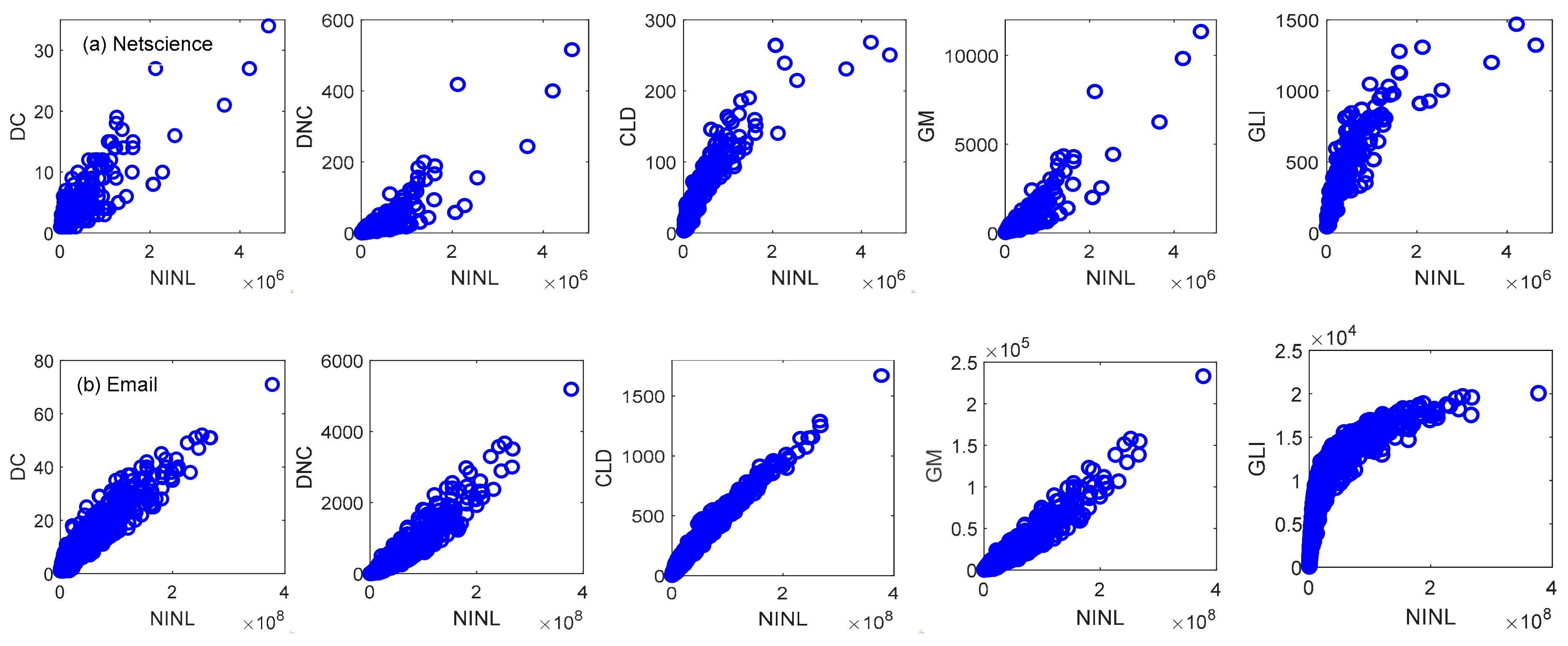
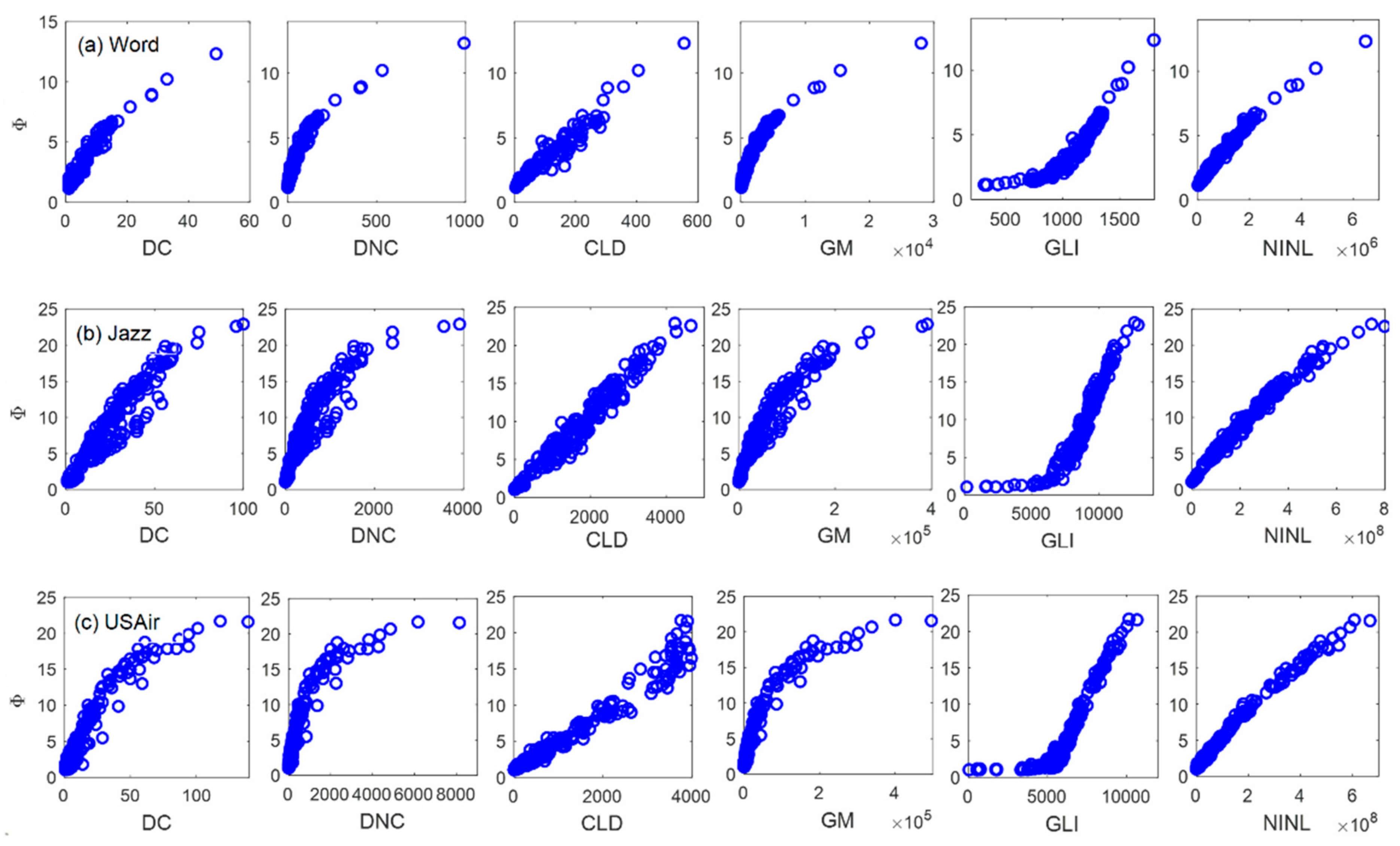
4.2.2. Influence Consistency Experiment

The influence consistency experiment was used to show the correlation between each method and the node influence and the correlation between the proposed method and each method. A higher correlation denotes a higher accuracy of node recognition. Figure 4 shows the experimental results of six methods on the Word, Jazz, and USAir networks. The x-axis is the node influence calculated by each method, and the y-axis is the node influence calculated by 1000 independent SIR spreading models. The experimental plots show that all six methods had positive correlations with node influence. Among them, the DNC and GM methods had an obvious upward convex trend, the GLI method had an obvious downward convex trend, and the DC, CLD, and NINL methods had a straight-line trend. The NINL method proposed in this paper showed better linearity in the three networks, and the scattered points were basically maintained around the straight line, suggesting a relatively strong correlation with the influence of nodes. In summary, the method proposed in this paper is more advantageous for discovering influential nodes.
To explore the intrinsic connection between the methods, Figure 5 shows the nodal influence correlation diagram between the proposed method and the other five methods in this paper. Each node in the figure represents the value obtained by a node in the network according to different methods. The x-axis refers to the NINL method values, and the y-axis refers to five method values of DC, DNC, CLD, GM, and GLI. As shown in Figure 5, the NINL method showed a positive correlation with the other five methods, and in the Netscience network, a more divergent scatter plot was obtained. In the Email network, the NINL method and CLD method seemingly presented a straight line. There was no such correlation when using the other methods. By observing the scatter plots of the NINL method and the DC method in the three networks, we can find that the value of DC method was concentrated in a very small interval, highlighting that the weak distinguishing ability of degree centrality for nodes was the main reason for the divergence of the results.

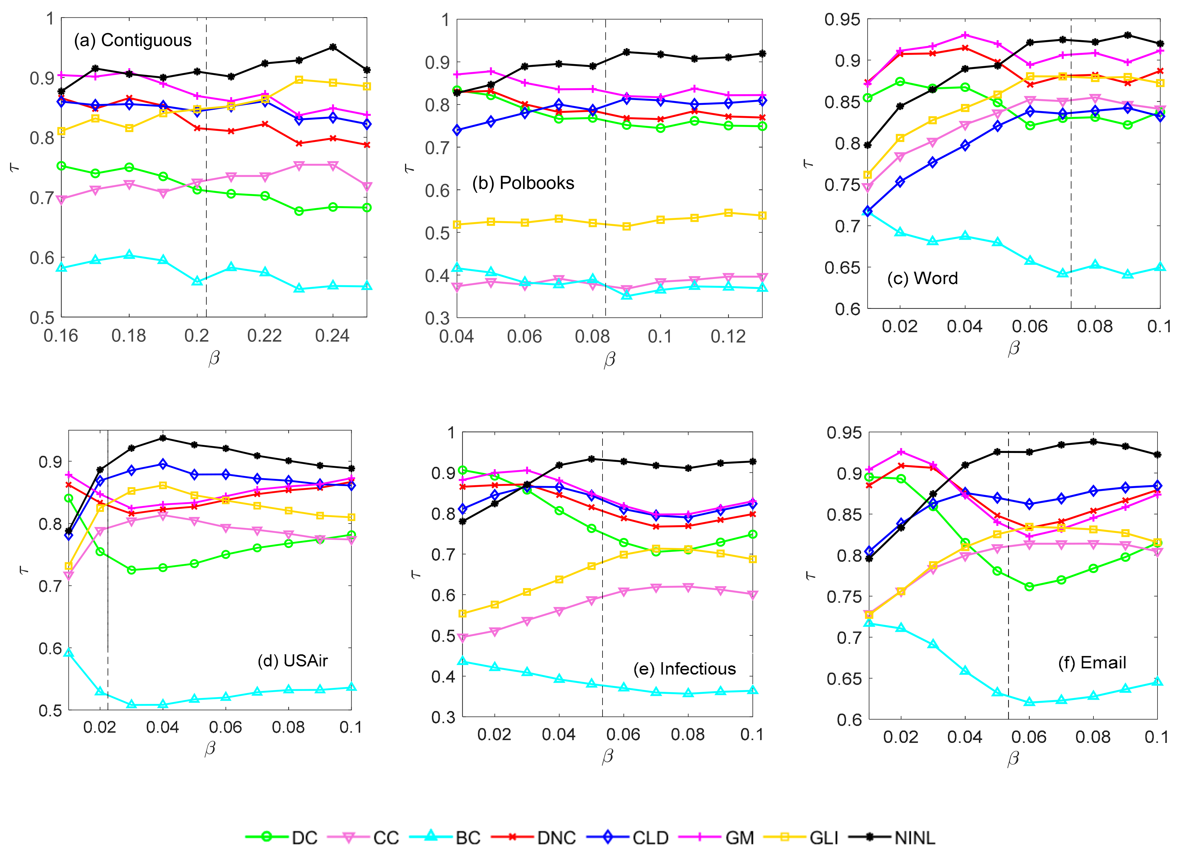
4.2.3. Recognition Effect of Each Method under a Certain Range of Propagation Probability

In order to more comprehensively evaluate the influence of the spreading probability on the ranking accuracy, this paper used the SIR model to obtain the node influence within a certain range of spreading probability, and the effectiveness of the proposed method was verified by the Kendall correlation coefficient. The results are shown in Figure 6. It can be seen from the figure that the BC method had the weakest ability to accurately identify influential nodes on the six networks. When the spreading probability was small, it can be seen that the DC, DNC, and GM methods had higher Kendall correlation coefficients, which was due to the fact that the infected node could only infect a portion of nodes close to it. At this time, the spreading process was limited to a certain local area, and the degree of a node in the local area had a great impact on the spreading influence. As the spreading probability was near the spreading threshold, the NINL method fully considered the relationship between the nearest neighbor and neighbor layer information within a certain range. Compared with other methods, NINL had a higher correlation with node influence, reflecting a better recognition effect. When the spreading probability was increased, we can see that the correlation curve had a significant decline in the USAir network. This is because the clustering coefficient of the network was very high, which led to the connection between nodes becoming closer. Under these circumstances, the information between nodes could be easily transmitted through the closely connected nodes layer by layer. As a result, the recognition accuracy of the NINL method approached that of the other methods. In general, the proposed NINL method could more accurately evaluate the influence of nodes than other methods around the propagation threshold.

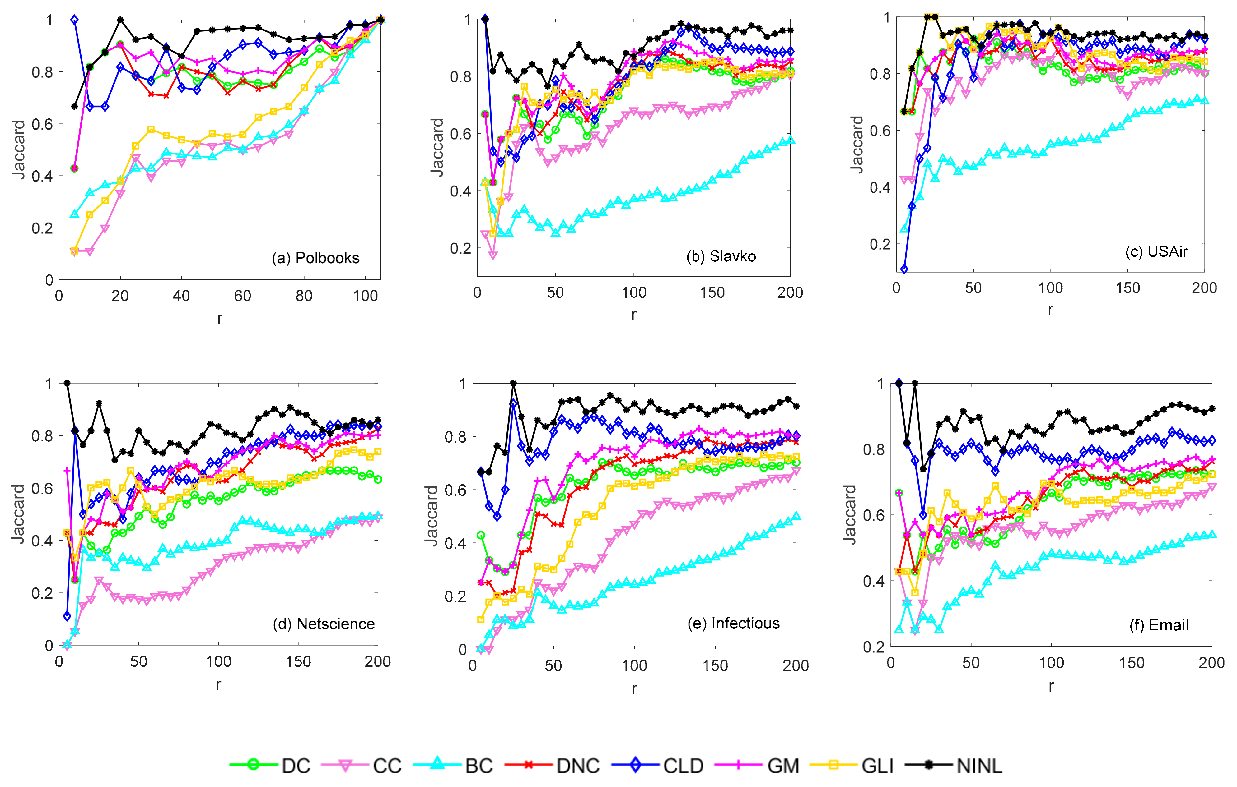
4.2.4. Recognition Effect of Each Method under a Certain Percentage of Ranking Results

There are a very small number of nodes in the network responsible for the normal operation of the entire network. It is of great significance to identify the most influential nodes. Table 4 shows the top 10 nodes obtained using each method in the Word and USAir networks. In this table, the Φ value given in the last column of the table is the ranking result calculated by the SIR model under the condition of spreading probability β. By observing the results of each method and the SIR model, it can be found that, in the Word network, the top 10 nodes identified by the DC, DNC, GM, GLI, and NINL methods had nine identical nodes in terms of Φ, whereas eight of the CC and CLD methods were identical. The BC method had only seven identical nodes. In the USAir network, the GM, GLI, and NINL methods identified nine identical nodes in terms of Φ, whereas DC and DNC only identified eight identical nodes, CC identified six identical nodes, and BC and CLD only identified five identical nodes. According to the above analysis, the NINL method could accurately identify the top 10 nodes.
In order to explore the recognition accuracy of the top nodes, the Jaccard similarity coefficient was used as the evaluation standard to carry out related experiments. Figure 7 presents the results of Jaccard similarity experiments on six types of networks. The x-axis represents the range of ranking results considered, and the y-axis represents the Jaccard similarity coefficient. A larger Jaccard coefficient denotes a higher similarity and, thus, a more effective recognition result. It can be seen from Figure 7 that, as the range of the ranking results increased, the Jaccard similarity coefficients obtained by each method became more and more stable. At the same time, the NINL method proposed in this paper clearly showed a superior similarity curve to the other seven methods in the Slavko, Netscience, Infectious, and Email networks. Thus, it can be considered that the NINL method was highly correlated with the influence of nodes and, thus, could more accurately identify the first r nodes.

5. Conclusions

In this paper, we studied the problem of identifying influential nodes in the network. Identifying influential nodes accurately in the network can provide a clearer understanding of the overall network function implementation process and the information dissemination between nodes. This paper mainly uses the symmetric adjacency matrix of the unweighted and undirected network to obtain various information. The paper first defines a node’s own information and neighbor layer nodes within a certain range as the initial node influence, and then takes the nearest neighbor information multiple times as the final influence of nodes. In different networks, the number of times to fetch the nearest neighbor information is different. In order to ensure the rationality of the p-value, a verification experiment of p selection was done. At the same time, this paper used the CCDF curve to perform a discrimination experiment on multiple real networks, while the Kendall coefficient and Jaccard similarity coefficient were used to carry out recognition and accuracy experiments. The method proposed in this paper effectively avoided the phenomenon of most nodes having the same value. Furthermore, it had higher accuracy in identifying the influence of nodes near the propagation threshold. The experimental results show that the proposed method was more effective than other methods in identifying influential nodes, which is significant for understanding the node information dissemination process.

Author Contributions

Conceptualization, J.Z. and L.W.; methodology, J.Z.; writing—original draft preparation, J.Z.; writing—review and editing, J.Z. All authors have read and agreed to the published version of the manuscript.

Funding

This research received no external funding.

Institutional Review Board Statement

Not applicable.

Informed Consent Statement

Not applicable.

Data Availability Statement

The datasets that support the findings of this study are openly available at https://github.com/Ismileo/Datasets, accessed on 19 July 2021.

Conflicts of Interest

The authors declare no conflict of interest.

References

  1. Pawan, K.; Ravins, D. Formalising and detecting community structures in real world complex networks. J. Syst. Sci. Complex. 2021, 34, 180–205. [Google Scholar]
  2. Robitaille, A.L.; Webber, Q.M.R.; Turner, J.W.; Wal, E.V. The problem and promise of scale in multilayer animal social networks. Curr. Zool. 2021, 67, 113–123. [Google Scholar] [CrossRef] [PubMed]
  3. Li, Q.; Jing, R.Z. Characterization of delay propagation in the air traffic network. J. Air Transp. Manag. 2021, 94, 102075. [Google Scholar] [CrossRef]
  4. Liu, Q.; Chen, Y.; Zhang, G.Q.; Wang, G.Y. A novel functional network based on three-way decision for link prediction in signed social networks. Cognit. Comput. 2021, 1–13. [Google Scholar] [CrossRef]
  5. Nguyen, T.; Le, H.; Quinn, T.P.; Nguyen, T.; Venkatesh, S. GraphDTA: Predicting drug–target binding affinity with graph neural networks. Bioinformatics 2021, 37, 1140–1147. [Google Scholar] [CrossRef] [PubMed]
  6. Freeman, L.C. Centrality in social networks conceptual clarification. Soc. Netw. 1978, 1, 215–239. [Google Scholar] [CrossRef] [Green Version]
  7. Freeman, L.C. A set of measures of centrality based on betweenness. Sociometry 1977, 40, 35–41. [Google Scholar] [CrossRef]
  8. Sabidussi, G. The centrality index of a graph. Psychometrika 1966, 31, 581–603. [Google Scholar] [CrossRef]
  9. Borgatti, S.P. Centrality and network flow. Soc. Netw. 2005, 27, 55–71. [Google Scholar] [CrossRef]
  10. Hwang, W.; Cho, Y.; Zhang, A.; Cho, Y.R.; Hwang, W. Bridging Centrality: Identifying Bridging Nodes in Scale-free Networks. In Proceedings of the Twelfth ACM SIGKDD International Conference on Knowledge Discovery and Data Mining (KDD’06), Philadelphia, PA, USA, 20–23 August 2006. [Google Scholar]
  11. Lü, L.Y.; Zhang, Y.C.; Yeung, C.H.; Zhou, T. Leaders in social networks, the Delicious case. PLoS ONE 2011, 6, e21202. [Google Scholar] [CrossRef] [Green Version]
  12. Kitsak, M.; Gallos, L.K.; Havlin, S.; Liljeros, F.; Muchnik, L.; Stanley, H.E.; Makse, H.A. Identification of influential spreaders in complex networks. Nat. Phys. 2010, 6, 888–893. [Google Scholar] [CrossRef] [Green Version]
  13. Lü, L.Y.; Zhou, T.; Zhang, Q.M.; Stanley, H.E. The H-index of a network node and its relation to degree and coreness. Nat. Commun. 2016, 7, 440–442. [Google Scholar] [CrossRef] [Green Version]
  14. Bae, J.; Kim, S. Identifying and ranking influential spreaders in complex networks by neighborhood coreness. Phys. A 2014, 395, 549–559. [Google Scholar] [CrossRef]
  15. Ahmed, I.; Mohamed, E.H. Density centrality: Identifying influential nodes based on area density formula. Chaos Solitons Fractals 2018, 114, 69–80. [Google Scholar]
  16. Li, Z.; Ren, T.; Ma, X.Q.; Zhou, T. Identifying influential spreaders by gravity model. Sci. Rep. 2019, 9, 355–359. [Google Scholar] [CrossRef] [PubMed] [Green Version]
  17. Li, M.T.; Zhang, R.S.; Hu, R.J.; Yang, F.; Yao, Y.; Yuan, Y.B. Identifying and ranking influential spreaders in complex networks by combining a local-degree sum and the clustering coefficient. Int. J. Mod. Phys. B 2018, 32, 1850118. [Google Scholar] [CrossRef]
  18. Sheng, J.F.; Dai, J.Y.; Wang, B.; Duan, G.H.; Long, J.; Zhang, J.K.; Guan, K.R.; Hu, S.; Chen, L.; Guan, W.H. Identifying influential nodes in complex networks based on global and local structure. Phys. A 2020, 541, 123262. [Google Scholar] [CrossRef]
  19. Yang, Y.Z.; Hu, M.; Huang, T.Y. Influential nodes identification in complex networks based on global and local information. Chin. Phys. B 2020, 29, 664–670. [Google Scholar] [CrossRef]
  20. Zareie, A.; Sheikhahmadi, A.; Jalili, M.; Fasaei, M.S.K. Finding influential nodes in social networks based on neighborhood correlation coefficient. Knowl. Based Syst. 2020, 194, 105580. [Google Scholar] [CrossRef]
  21. Yan, X.L.; Cui, Y.P.; Ni, S.J. Identifying influential spreaders in complex networks based on entropy weight method and gravity law. Chin. Phys. B. 2020, 29, 664–672. [Google Scholar] [CrossRef]
  22. Babu, M.; Marimuthu, S.; Joy, M.; Nadaraj, M.; Jeyaseelan, L. Forecasting COVID-19 epidemic in India and high incidence states using SIR and logistic growth models. Clin. Epidemiol. Glob. Health 2021, 9, 26–33. [Google Scholar]
  23. Kermack, W.O.; McKendrick, A.G. A contribution to the mathematical theory of epidemics. Proc. R. Soc. A 1927, 115, 700–721. [Google Scholar]
  24. Contiguous USA Network Dataset—KONECT. 2017. Available online: http://konect.cc/networks/contiguous-usa (accessed on 5 July 2021).
  25. Lusseau, D.; Schneider, K.; Boisseau, O.J.; Haase, P.; Slooten, E.; Dawson, S.M. The bottlenose dolphin community of Doubtful Sound features a large proportion of long-lasting associations. Behav. Ecol. Sociobiol. 2003, 54, 396–405. [Google Scholar] [CrossRef]
  26. Blagus, N.; Šubelj, L.; Bajec, M. Self-similar scaling of density in complex real-world networks. Phys. A 2012, 391, 2794–2802. [Google Scholar] [CrossRef] [Green Version]
  27. Newman, M.E.J. Finding community structure in networks using the eigenvectors of matrices. Phys. Rev. E 2006, 74, 036104. [Google Scholar] [CrossRef] [PubMed] [Green Version]
  28. Gleiser, P.M.; Danon, L. Community structure in jazz. Adv. Complex Syst. 2003, 6, 565–573. [Google Scholar] [CrossRef] [Green Version]
  29. Batagel, V.; Mrvar, A. Pajek-program for large Network analysis. Connections 1998, 21, 47–57. [Google Scholar]
  30. Isella, L.; Stehlé, J.; Barrat, A.; Cattuto, C.; Pinton, J.F.; Broeck, W.V.D. What’s in a crowd? Analysis of face-to-face behavioral networks. J. Theor. Biol. 2011, 271, 166–180. [Google Scholar] [CrossRef] [Green Version]
  31. Guimerà, R.; Danon, L.; Díaz, G.A.; Giralt, F.; Arenas, L. Self-similar community structure in a network of human interactions. Phys. Rev. E 2003, 68, 065103. [Google Scholar] [CrossRef] [Green Version]
  32. Datasets. Available online: https://github.com/Ismileo/Datasets (accessed on 19 July 2021).
  33. Newman, M.E.J. Assortative mixing in networks. Phys. Rev. Lett. 2002, 89, 208701. [Google Scholar] [CrossRef] [Green Version]
  34. Castellano, C.; Pastor-Satorras, R. Thresholds for epidemic spreading in networks. Phys. Rev. Lett. 2010, 105, 218701. [Google Scholar] [CrossRef] [Green Version]
  35. Knight, W.R. A computer method for calculating kendall’s tau with ungrouped data. J. Am. Stat. Assoc. 1966, 61, 436–439. [Google Scholar] [CrossRef]
  36. Lorentz, J.; Bolboacă, S.-D. Pearson versus Spearman, Kendall’s Tau Correlation Analysis on Structure-Activity Relationships of Biologic Active Compounds. Leonardo J. Sci. 2006, 5, 179–200. [Google Scholar]
  37. Amirkhani, D.; Bastanfard, A. An objective method to evaluate exemplar-based inpainted images quality using Jaccard index. Multimed. Tools. Appl. 2021, 80, 26199–26212. [Google Scholar] [CrossRef]
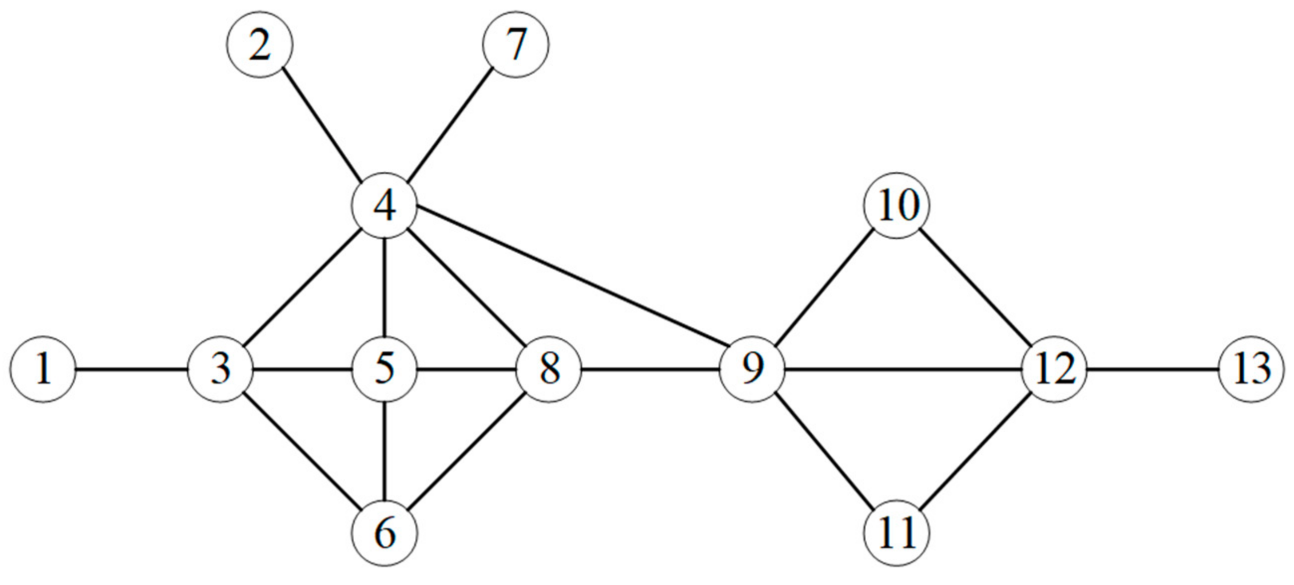
Figure 1. Example network.
Symmetry 13 01570 g001
Figure 2. CCDF of the ranking results obtained using each method. (af): CCDF on the network of Contiguous, Dolphin, Jazz, Slavko, Infectious, Email.
Symmetry 13 01570 g002
Figure 3. Kendall values of different p-values on 10 networks.
Symmetry 13 01570 g003
Figure 4. The correlation between six methods and the influence of nodes by SIR model on three networks. (ac): The correlation on the network of Word, Jazz, USAir.
Symmetry 13 01570 g004
Figure 5. The correlation between several methods and the proposed method on two networks. (a,b): The correlation on the network of Netscience, Email.
Symmetry 13 01570 g005
Figure 6. Accuracy comparison of different methods under different probabilities. (af): The Kendall correlation coefficient on the network of Contiguous, Polbooks, Word, USAir, Infectious, Email.
Symmetry 13 01570 g006
Figure 7. Comparison of Jaccard similarity of different methods. (af): The Jaccard similarity on the network of Polbooks, Slavko, USAir, Netscience, Infectious, Email.
Symmetry 13 01570 g007
Table 1. Node influence calculation results of the example network.
Node12345678910111213
NINL029373738373737383837373724
NINL1373814122415011238150187757513637
NINL2141224523704627441224673660323323374136
NINL3523704191329312341182370424322397103410341442374
Table 2. Basic topological characteristics of 10 real networks.
Networksnmkmax<k>DLCr
Contiguous4910784.367114.1630.4970.2334
Dolphins62159125.12983.3570.259−0.0436
Polbooks105441258.473.0790.488−0.1279
Word112425497.58952.5360.173−0.1293
Jazz198274210027.69762.2350.6180.0202
Slavko32422185813.69173.0540.4660.2473
USAir332212613912.80762.7380.625−0.2079
Netscience379914344.823176.0420.741−0.0817
Infectious41027655013.48893.6310.4560.2258
Email11335451719.62283.6060.2200.0782
Table 3. Kendall coefficient between ranking list obtained by SIR model and by other methods using 10 networks.
NetworksβthβτDCτCCτBCτDNCτCLDτGMτGLIτNINL
Contiguous0.20270.200.71260.72530.55870.81550.84350.86900.84690.9099
Dolphin0.14700.150.77210.61870.53890.83550.79160.87310.83550.9344
Polbooks0.08380.090.75180.36790.35050.76790.81390.81980.51410.9229
Word0.07260.080.83110.85490.65230.88220.83880.90860.87840.9218
Jazz0.02590.030.80690.70800.45690.81750.86550.85050.89370.9322
Slavko0.04660.050.77190.71280.36250.82340.85380.84110.79380.9305
USAir0.02250.030.72510.80430.50810.81570.88540.82430.85220.9211
Netscience0.12470.130.59550.32920.30480.77240.79800.77880.69500.8395
Infectious0.05340.060.72810.60950.37070.78770.81050.81860.69840.9273
Email0.05350.060.76150.81380.62030.83300.86220.82260.83450.9255
Table 4. Top 10 nodes measured using various methods in Word and USAir networks.
Word NetworkUSAir Network
RankDCCCBCDNCCLDGMGLININLΦRankDCCCBCDNCCLDGMGLININLΦ
11818181818181818181118118118118109118118118261
233333333322612618261131261261261118
3445244525252525252325567261255112255255255255
45244524444444444444152255201182299182182182182
5105281010551105105105105518220147152118152152152230
6101058010105102551106230182182230255230230230176
7251010528222551102571664725516617616667112152
82827282555512826518671661526714767166166147
95125251252826252891122483131122611121126767
10226292632261055551020111213201301147147147166
Publisher’s Note: MDPI stays neutral with regard to jurisdictional claims in published maps and institutional affiliations.

