A General Model for Describing the Ovate Leaf Shape

Abstract

Many plant species produce ovate leaves, but there is no general parametric model for describing this shape. Here, we used two empirical nonlinear equations, the beta and Lobry–Rosso–Flandrois (LRF) equations, and their modified forms (referred to as the Mbeta and MLRF equations for convenience), to generate bilaterally symmetrical curves along the x-axis to form ovate leaf shapes. In order to evaluate which of these four equations best describes the ovate leaf shape, we used 14 leaves from 7 Neocinnamomum species (Lauraceae) and 72 leaves from Chimonanthus praecox (Calycanthaceae). Using the AIC and adjusted root mean square error to compare the fitted results, the modified equations fitted the leaf shapes better than the unmodified equations. However, the MLRF equation provided the best overall fit. As the parameters of the MLRF equation represent leaf length, maximum leaf width, and the distance from leaf apex to the point associated with the maximum leaf width along the leaf length axis, these findings are potentially valuable for studying the influence of environmental factors on leaf shape, differences in leaf shape among closely related plant species with ovate leaf shapes, and the extent to which leaves are bilaterally symmetrical. This is the first work in which temperature-dependent developmental equations to describe the ovate leaf shape have been employed, as previous studies lacked similar leaf shape models. In addition, prior work seldom attempted to describe real ovate leaf shapes. Our work bridges the gap between theoretical leaf shape models and empirical leaf shape indices that cannot predict leaf shape profiles.

1. Introduction

The ovate leaf shape is a common geometric form among many plant species, especially in the Lauraceae. It therefore exists in almost all floras. Similar linear leaf forms with comparable structural characteristics occur in other widely spread flowering plant families. However, there is no strict distinction between these two leaf shapes, although the difference between these two kinds of shapes comes from the variation in the ratio of leaf width to leaf length [1,2,3]. Previous studies show that a simplified version of a polar coordinate equation (proposed by Gielis [4]) can describe all shapes of bamboo leaves, including narrow linear leaves and even some with approximate ovate shapes [5,6]. However, variations in the general ovate shape occur as a result of subtle changes in the curvature along the leaf margin from the leaf apex to the point of the maximum leaf width. These variations limit the utility of the simplified Gielis equation in generically describing the ovate leaf shape [1,7].

In order to address these biological variations in leaf form mathematically, we employed the beta equation [8] and the Lobry–Rosso–Flandrois (LRF) equation [9,10]. These equations have two significant advantages: (i) they provide a better goodness of fit than other equations, and (ii) their four-parameter space reflects a better close-to-linear behavior for a nonlinear fit [11,12]. These two equations can generate curves that look like one side of an ovate leaf (as defined by the midrib running along the length of the leaf lamina). Importantly, the four parameters in each of these two equations can be shown to correspond to half of the maximum leaf width, the point on the leaf length axis associated with the leaf maximum width, the leaf base that connects the lamina and the petiole, and the leaf apex. These parameters, especially the first two, are especially meaningful for describing the shapes of ovate leaves. Specifically, the ratio of the distance from leaf apex to the point on the leaf length axis associated with leaf maximum width and total leaf length can be used to study the evolution and variation in leaf shape, even among distantly related species [13]. In addition, Shi et al. [14] proposed more general forms for the beta and LRF equations by introducing an additional parameter for each equation, which makes both equations more flexible and morphologically versatile.

Although some parametric leaf shape models exist, these models focus on linear leaves, especially those of crops and bamboos [5,6,15]. Here, we further modify the beta and LRF equations and apply their modified forms to generate ovate leaf shapes and test their utility by examining the leaves of seven species (including a variety) of the genus Neocinnamomum (Lauraceae). These species have typical ovate leaves that are morphologically representative of the general ovate leaf form of many other species (e.g., Prunis). In addition, to test whether an additional parameter is valuable in the modified beta and modified LRF equations, we used 72 individual leaves from the species Chimonanthus praecox (Calycanthaceae) to examine the goodness of fit and its trade-off with model complexity. Previously, it was shown that similar models were useful for fitting temperature-dependent developmental rates of arthropods [12] and the ontogenetic growth of plants [8,14]. If our four models could be demonstrated to be valid in describing the actual ovate leaf shapes of a plant group, it would show that these models have a wider scope in applications, and further suggest that there probably exists a similar mechanism for ontogenetic development and growth.

In this study, we aim to build several new leaf shape models that can describe ovate leaves and to find whether there is a best one relative to other candidate models. This work does not recommend a leaf shape index such as the leaf roundness index and leaf dissection index [16,17,18,19,20], because a leaf shape index cannot be used to fit the edge data of ovate leaves. Here, the mathematical model that we finally recommend can describe the ovate leaf shape with model parameters that can be well understood. In addition, the model parameters can be used to quantify leaf shape (see the Materials and Methods section for details). Although leaf shape can be affected by environmental factors [21,22], we did not attempt to check the influences of environmental factors on leaf shape, which exceeded the scope of the current study, but deserves future study.

2. Materials and Methods

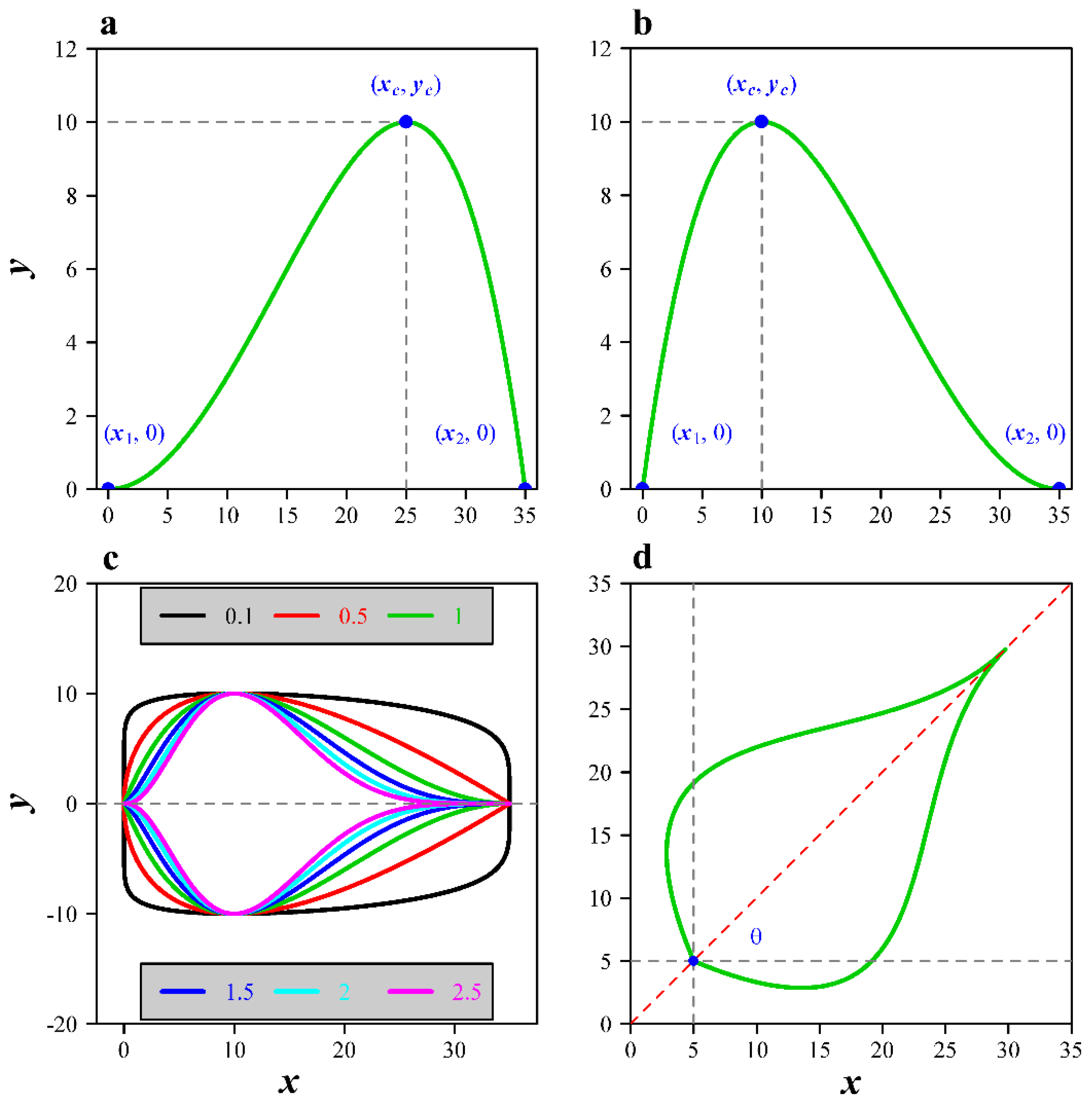
2.1. Models

The original beta and Lobry–Rosso–Flandrois (LRF) equations, which have been used to describe the influence of temperature on the growth rate of crops and bacteria and the developmental rates of insects, produce similar left-skewed curves in the range between the lower and upper developmental thresholds (Figure 1a). Each has four parameters with the same or very similar geometric meanings [8,9,10]. Specifically, the

Beta equation is:

$$y=y_c\left(\frac{x_2-x}{x_2-x_c}\right){\left(\frac{x-x_1}{x_c-x_1}\right)}^{\frac{x_c-x_1}{x_2-x_c}},$$

(1)

and the LRF equation is:

$$y=\frac{y_c\left(x-x_2\right){\left(x-x_1\right)}^2}{\left(x_c-x_1\right)\left[\left(x_c-x_1\right)\left(x-x_c\right)-\left(x_c-x_2\right)\left(x_c+x_1-2x\right)\right]},$$

(2)

where y represents the developmental rate at temperature x; y_c represents the maximum developmental rate; x_c represents the temperature associated with the maximum developmental rate y_c; x₁ and x₂ represent the lower and upper developmental thresholds that are the left and right intersections of the curve and the x-axis (Figure 1a). The beta equation can produce left- or right-skewed curves, whereas the LRF equation produces only left-skewed curves. When using the leaf base as the starting point and the leaf apex as the ceiling point, another form of the LRF equation should be used [14], i.e.,

$$y=\frac{y_c\left(x-x_1\right){\left(x-x_2\right)}^2}{\left(x_2-x_c\right)\left[\left(x_2-x_c\right)\left(x-x_c\right)-\left(x_1-x_c\right)\left(x_c+x_2-2x\right)\right]}.$$

(3)

Equation (3) is actually symmetrical with Equation (2) around the vertical axis x = (x₁ + x₂)/2 (Figure 1b). To increase the flexibility of curve fitting, Shi et al. [14] proposed generalized versions of the beta and LRF equations, i.e.,

Modified Beta equation:

$$y=y_c{\left[\left(\frac{x_2-x}{x_2-x_c}\right){\left(\frac{x-x_1}{x_c-x_1}\right)}^{\frac{x_c-x_1}{x_2-x_c}}\right]}^{\delta },$$

(4)

Modified LRF equation:

$$y=y_c{\left[\frac{\left(x-x_1\right){\left(x-x_2\right)}^2}{\left(x_2-x_c\right)\left[\left(x_2-x_c\right)\left(x-x_c\right)-\left(x_1-x_c\right)\left(x_c+x_2-2x\right)\right]}\right]}^{\delta },$$

(5)

where δ is an additional parameter, the numerical value of which influences the curvature of the curve. To reduce the model’s complexity in the current study, x₁ was fixed to be zero. An ovate leaf shape can be generated by defining a symmetrical equation along the x-axis for Equations (4) and (5): $f(x)=y(x)$ and $g(x)=-y(x)$, where f(x) and g(x) represent the upper and lower parts of the leaf shape curve, respectively. Figure 1c shows simulated leaf shape curves with different δ values. Hereafter, for convenience, we refer to Equations (4) and (5) as the Mbeta and MLRF equations.

For each of the four models, the parameters can be used to quantify leaf shape characteristics. For instance, the ratio of x_c to x₂ can reflect whether the maximum leaf width is more approximate to the middle of the lamina, and the ratio of 2y_c to x₂ approximates the ratio of lamina width to length.

2.2. Parameter Estimation for the Models

The coordinates of the leaf edge can be obtained by scanning leaf profile images [1]. The coordinates of the leaf base are not exactly located at (0, 0), and the angle between the leaf length axis (i.e., a straight line through leaf base and leaf apex) and the x-axis is usually not equal to 0 (Figure 1d). Thus, to obtain the estimates of the model parameters, three additional parameters are required, i.e., x₀, y₀, and θ, where (x₀, y₀) represent the coordinates of the leaf base, and θ is the angle between the aforementioned two axes. Thus, for the beta and LRF equations, there are six parameters in total (i.e., three location parameters plus three model parameters); for the Mbeta and MLRF equations, there are seven parameters in total (i.e., three location parameters plus four model parameters). The residual sum of squares (RSS) of the y coordinate was used to measure the goodness of fit:

$$\mathrm{RSS}={\displaystyle {\sum }_{i=1}^n{\left(y_i-{\widehat{y}}_i\right)}^2},$$

(6)

where i denotes the ith point on the leaf edge; n denotes the number of data points on the leaf edge; and y_i with a circumflex denotes the predicted value of y_i using a nonlinear equation. To reflect the trade-off between the goodness of fit and the model’s complexity, the Akaike information criterion (AIC) was also calculated [23]:

$$\mathrm{AIC}=2p+n\left[\ln \left(2\pi \right)+1-\ln \left(n\right)+\ln \left(\mathrm{RSS}\right)\right],$$

(7)

where p is the number of model parameters plus an error item. The equation with the lowest AIC is considered as the best one.

To diminish the influence of leaf size on the RSS, we used the adjusted root mean square error (RMSE_adj) (see References [24,25]) to intuitively compare the goodness of fit for different leaves:

$${\mathrm{RMSE}}_{\mathrm{adj}}=\frac{\sqrt{\mathrm{RSS}/n}}{\sqrt{A/\pi }},$$

(8)

where A denotes the leaf area. The adjusted RMSE accounts for the proportion of the average absolute deviation in the y coordinate to the radius of an assumed circle whose area is equal to the leaf area, and this is used as a reference indicator during the comparison of models.

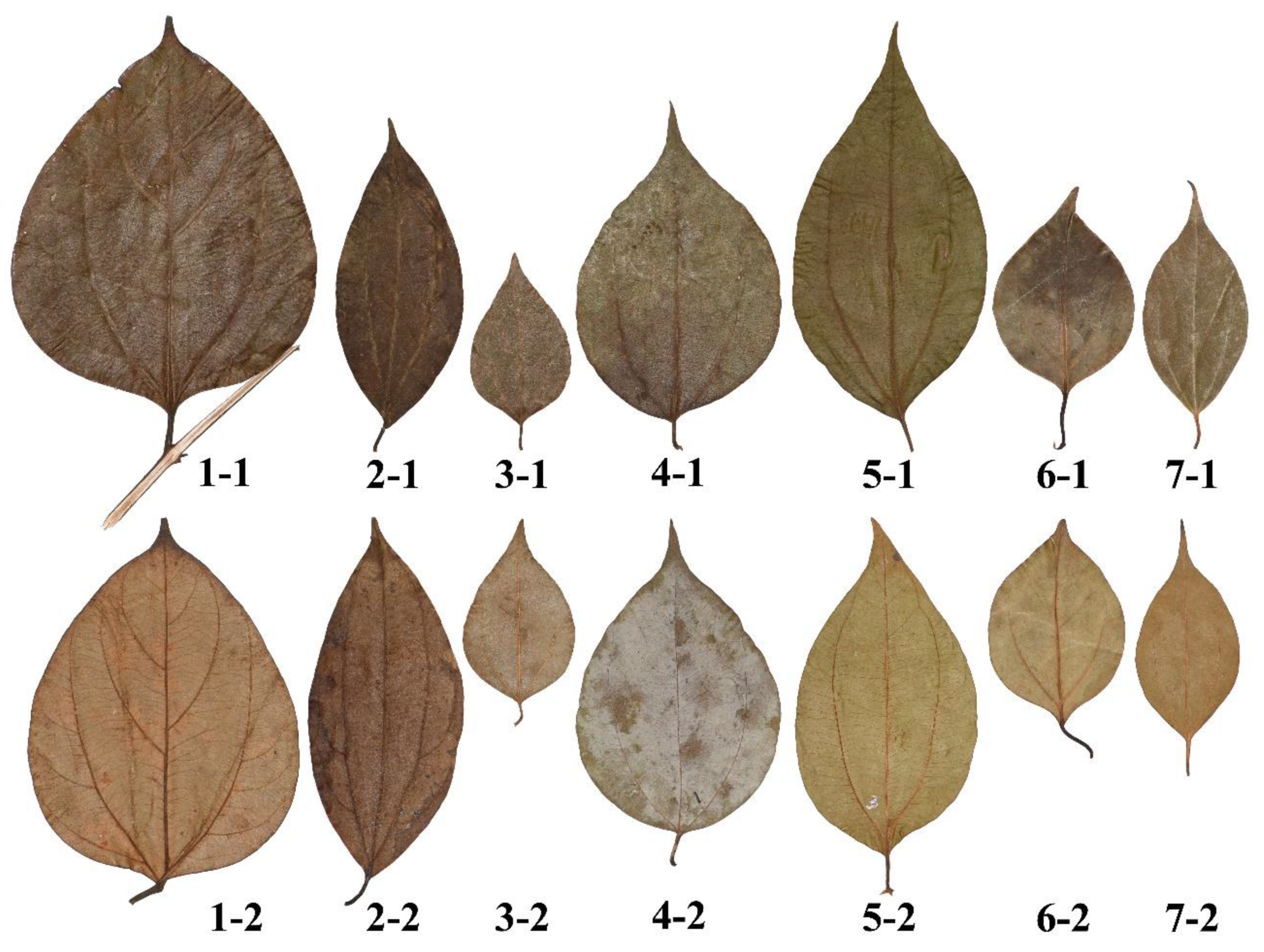
2.3. Samples of Representative Ovate Leaves

Representative plants of Neocinnamomum (Lauraceae) species with representative ovate leaf shapes were used to determine which among the four candidate equations provided the best fit. The leaves were collected from southern China, where the plants grew naturally (

Table 1. Sampling information for the Neocinnamomum leaves.

Code	Latin Name	Locality	Longitude (°), Latitude (°)	Sampling Date
1	Neocinnamomum lecomtei H. Liu	Hainan, China	107.8394, 22.4641	2017.03.09
2	Neocinnamomum complanifructum S.K. Lee et F.N. Wei	Yunnan, China	104.0189, 22.4669	2017.10.09
3	Neocinnamomum fargesii (Lecomte) Kosterm.	Sichuan, China	110.2984, 31.3034	2017.02.20
4	Neocinnamomum delavayi (Lecomte) H. Liu	Sichuan, China	103.9540, 28.5396	2017.09.04
5	Neocinnamomum caudatum (Nees) Merr.	Hainan, China	98.2949, 24.8070	2017.05.08
6	Neocinnamomum caudatum (Nees) Merr. var. macrocarpum W.B. Xu et B.S. Xia	Guangxi, China	106.3458, 23.5951	2017.11.17
7	Neocinnamomum mekongense (Hand.-Mazz.) Kosterm.	Yunnan, China	99.9285, 24.5804	2017.05.08

). Two healthy and mature representative leaves from each species were collected (Figure 2). To further compare the four candidate equations, we used 72 leaves of Chimonanthus praecox (Calycanthaceae) growing in the Nanjing Forestry University campus collected on 20 October 2017. There is no evidence to show that the geographical location, plant age, leaf position in the canopy, or light conditions can significantly alter the basic leaf shape characteristics of ovate leaves. Thus, we randomly sampled leaves from the plants that we had access to. Under any circumstances, any significant change in leaf shape would have no effect on evaluating which equation best described leaf shape. Indeed that is the whole point of this study.

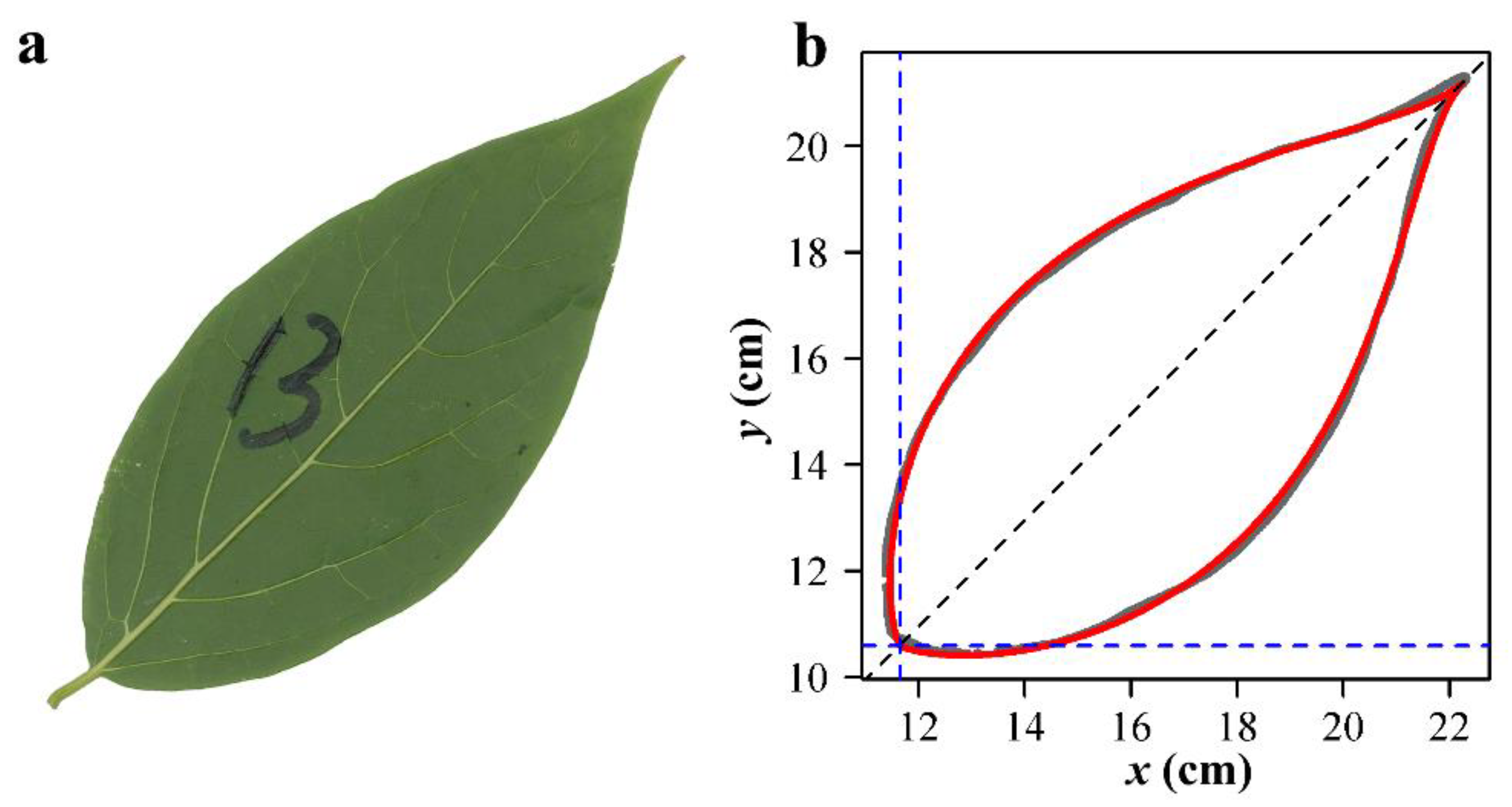
2.4. Leaf Image Processing and Data Acquisition

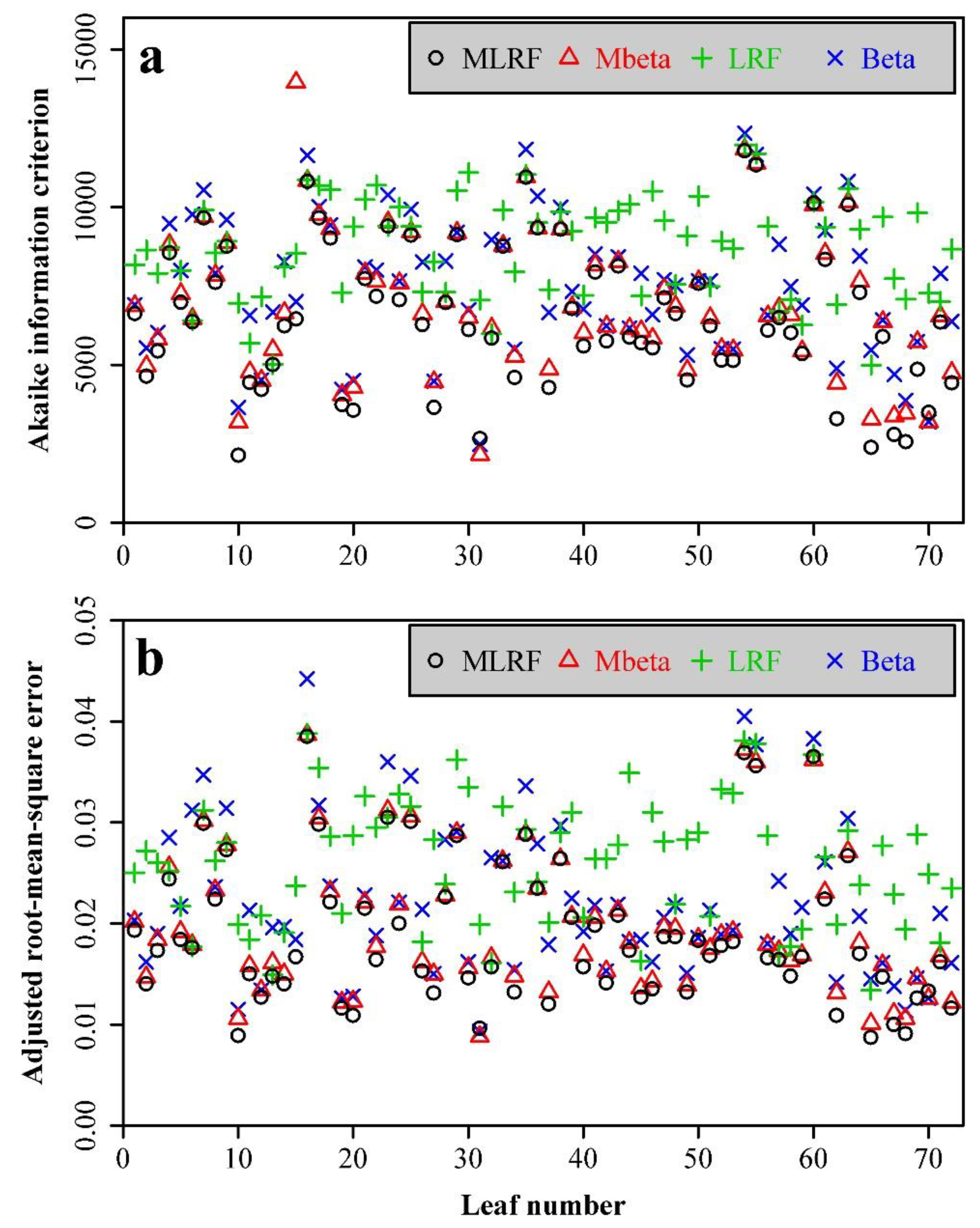
The Neocinnamomum leaves were photographed in jpg format, and the leaves of C. praecox were scanned using a photo scanner (HP Scanjet 4850; Hewlett-Packard Company, Palo Alto, California) at 400 dpi resolution. A Matlab procedure (version ≥ 2009a) [1] was used to extract planar coordinates for each leaf. The numbers of data points on the leaf edge for the 14 Neocinnamomum specimens ranged from 1000 to 2700 depending on the leaf size; the data points of the leaves of C. praecox were set to be ca. 3000. These numbers of data points are sufficient to form an integrated leaf shape. Each leaf image was transferred to a black–white image in bmp format. We fitted the four candidate equations (i.e., the beta, LRF, Mbeta and MLRF equations) to the leaf shape data using the Nelder–Mead optimization method [26], which was carried out using the “optim” function in R software (version 3.6.1) [27]. The target function is the RSS (see Equation (6) for details).

3. Results

For the 14 Neocinnamomum leaf specimens, the Mbeta and MLRF equations provided better fits than the beta or LRF equations. Specifically, 11 out of 14 AIC and RMSE_adj values of the MLRF equation were smaller than those using the Mbeta equation (

Table 2. The AICs and adjusted root mean square errors using the four equations for the 14 Neocinnamomum leaf specimens.

Leaf No.	Beta		Mbeta		LRF		MLRF
	AIC	RMSEadj	AIC	RMSEadj	AIC	RMSEadj	AIC	RMSEadj
1-1	6158	0.0288	6119	0.0286	9288	0.0522	6240	0.0292
1-2	4947	0.0279	4467	0.0252	8623	0.0599	4552	0.0256
2-1	2508	0.0375	1968	0.0320	1998	0.0323	1940	0.0318
2-2	4013	0.0384	3774	0.0362	3712	0.0357	3712	0.0357
3-1	277	0.0372	−653	0.0232	−607	0.0238	−648	0.0232
3-2	349	0.0342	−702	0.0209	−621	0.0218	−723	0.0207
4-4	4587	0.0448	4425	0.0429	4664	0.0457	4380	0.0424
4-2	1037	0.0179	1035	0.0179	3816	0.0364	675	0.0163
5-1	4302	0.0309	2647	0.0215	2617	0.0214	2597	0.0213
5-2	3933	0.0378	3490	0.0337	3678	0.0354	3423	0.0331
6-1	1211	0.0379	999	0.0348	973	0.0345	936	0.0339
6-2	1189	0.0376	1165	0.0372	1293	0.0392	1136	0.0367
7-1	86	0.0265	−294	0.0229	−481	0.0213	−483	0.0213
7-2	489	0.0333	53	0.0280	7	0.0275	−8	0.0273

). This result was interpreted to indicate that the MLRF equation is the best model among the other candidate equations. The adjusted RMSE values using the MLRF equation for the 14 leaves ranged from 0.0163 to 0.0424, i.e., the average absolute deviation of the curve fitting was less than 5% of the radius of a circle, assuming that its area is equal to the leaf area. This result further validated the superiority of the MLRF equation for describing ovate leaf shapes. Figure 3 shows the fitted results using the MLRF equation.

The MLRF equation was also found to be the best one among the four candidate equations based on the 72 individual leaves collected from C. praecox (Figure 4a). Specifically, the AIC values of the Mbeta equation were greater than those of the MLRF equation for 67 out of 72 leaves. In addition, the adjusted RMSE values of the Mbeta equation were greater than those of the MLRF equation for the same number of leaves (Figure 4b). The adjusted RMSE values using the MLRF equation for the 72 leaves ranged from 0.0087 to 0.0385, indicating that the average absolute deviation of the curve fitting was less than 4% of the radius of a circle whose area is hypothesized to equal the leaf area. The MLRF equation fitted the leaf edge data of C. praecox well (see Figure 5 for example).

Tables S1 and S2 in the online Supplementary Materials tabulate the estimates of the model parameters and the goodness of fit for the 86 leaves (14 + 72).

4. Discussion

Dornbusch et al. [15] proposed an empirical model to describe the leaf shapes of several crop species (i.e., Triticum aestivum, Hordeum vulgare and Zea mays cultivars). The advantage of this model is that it only requires information pertaining to leaf length, leaf maximum width, and the ratio of the distance from the leaf apex to the point on the leaf length axis associated with the leaf maximum width. However, this model consists of two step functions (i.e., from the leaf apex to the leaf maximum width and from the leaf maximum width to leaf base), which does not necessarily lead to smoothness at the junction between the two step functions (i.e., the point on the leaf edge curve at which the leaf has its maximum width). Shi et al. [5] proposed a simplified version of generating leaf shapes based on the original Gielis equation [4] using three location parameters and two model parameters. The modified Gielis equation can produce a similar but smoother curve than that of Dornbusch et al. [15], and it has fewer parameters (only two model parameters). Lin et al. [6] tested the validity of the simplified Gielis equation using the leaves of 42 bamboo species, and found that the equation fit them well. However, the simplified Gielis equation cannot produce a concave curve close to the leaf apex, the same limitation as that of the equation of Dornbusch et al. [15].

In contrast, the curve produced by the MLRF equation presented here not only produces an ovate leaf shape similar to that produced by the simplified Gielis equation (see Figure 1c for the case of δ = 0.5), but it also produces a concave curve close to the leaf apex. If an ovate leaf is not strictly bilaterally symmetrical for the parts close to the leaf apex (e.g., when one side is a linear or convex curve, whereas the other side is a concave curve), more parameters can be set for one or the other side (e.g., two δ values can be fitted, one for each side of the leaf). Thus, the MLRF equation can describe a broad variety of ovate leaf shapes. For some linear leaf shapes that have the same structural characteristics as ovate leaf shapes but a lower y_c value in the MLRF equation, the MLRF equation is still applicable, because there is no strict distinction between an ovate leaf shape and a linear leaf shape of the other kind. Schrader et al. [3] distinguished between the two leaf forms using the ratio of leaf width to leaf length, such that leaf shapes with ≤1/10 width/length ratio are defined as linear rather than ovate. Although this is an empirical definition, it shows that an ovate leaf shape can be defined as a linear leaf shape with a lower ratio of leaf width to length. Clearly, there are other linear leaf shapes that have structural characteristics that differ from the ovate leaf shape, i.e., linear leaf shapes appear to be similar because the small ratio of leaf width to length has hidden their different structural characteristics. However, these linear forms probably result from other leaf shapes that have been described as acicular, acuminate, cuneate, deltoid, or elliptical shapes. Examining these forms using the approach described here merits further investigation.

An important limitation of the MLRF equation is that its ability to mimic ovate shapes manifests errors at the leaf apex that can be large for some leaves (Figure 3). The actual leaf apex is longer and more skewed compared to the predicted form. This likely results from the evolution of what is called a drip-point in some Lauraceae species that can quickly drain water from the leaf surface (for a discussion of this phenomenon, see ref. [28]). We believe that this process-driven mechanism may be similar to temperature-dependent growth dynamics [29,30,31]. The process of leaf size growth has been demonstrated to follow a sigmoid curve [32]. According to References [8,14], a sigmoid curve results from integrating the beta equation or the LRF equation. Thus, the growth rate of a leaf results in curves that can still be simulated by the MLRF equation.

There are many statistical approaches, especially non-parametric models, such as elliptic Fourier, kernel estimation, local regression, neural network, and spline [33,34], which can depict leaf shape very accurately. However, these approaches have significant disadvantages such as requiring too many parameters in each step of multi-step calculations [33], and biologically important shape parameters fail to appear in these non-parametric approaches. In comparison with these models, the Mbeta and MLRF equations provide clear geometric and biological analogs for the curves they generate. For example, x_c represents the point on the leaf length axis associated with half of the leaf maximum width (i.e., y_c), x₂ represents leaf length, and δ can be used to adjust the concavity and convexity of a curve. There are other advantages of using the Mbeta and MLRF equations over other nonlinear temperature-dependent developmental rate equations such as the Briére, Lactin and square root equations [35,36,37,38]. In these models, with the exception of the lower and upper thresholds (i.e., x₁ and x₂), there are other parameters that cannot directly provide a link to a curve’s shape. However, the parameters in the MLRF equation can be intuitively understood and used to quantify the complexity of leaf shape. It can be used to assess leaf shape differences among different individuals of the same species or among different species that are taxonomically closely or distantly related. In addition, the MLRF equation, which generates bilaterally symmetrical leaf shapes perfectly, can be used to quantify the extent of bilateral asymmetry.

5. Conclusions

The modified beta and LRF equations (i.e., the Mbeta and MLRF equations) are demonstrated to be more flexible for data fitting than their original versions (the beta and LRF equations), and the MLRF equation has a lower AIC or adjusted RMSE value than the Mbeta equation for most of the data sets studied here. The MLRF equation can generate two types of ovate leaf shapes: for the part of the curve from the leaf apex to a point on the leaf edge not reaching the leaf maximum width (wherein one type is approximately linear and somewhat convex), and the other is concave. The MLRF appears to be more useful than other available leaf morphometric models for describing ovate leaf shapes. For example, the ratios of the average absolute deviation in the y coordinate to the radius of the assumed circle whose area equals leaf area are smaller than 5% for all leaves investigated. In addition, with the exception of δ, the other parameters of the MLRF can be intuitively understood in terms of geometric and biological features. Thus, the work presented has potential value for future studies understanding the influence of environmental factors on leaf shape for plants with ovate leaf shapes.

References

1. Shi, P.; Ratkowsky, D.A.; Li, Y.; Zhang, L.; Lin, S.; Gielis, J. General leaf-area geometric formula exists for plants—Evidence from the simplified Gielis equation. Forests 2018, 9, 714. [Google Scholar] [CrossRef] [Green Version]
2. Gallaher, T.J.; Adams, D.C.; Attigala, L.; Burke, S.V.; Craine, J.M.; Duvall, M.R.; Klahs, P.C.; Sherratt, E.; Wysocki, W.P.; Clark, L.G. Leaf shape and size track habitat transitions across forest–grassland boundaries in the grass family (Poaceae). Evolution 2019, 73, 927–946. [Google Scholar] [CrossRef] [PubMed]
3. Schrader, J.; Shi, P.; Royer, D.L.; Peppe, D.J.; Gallagher, R.V.; Li, Y.; Wang, R.; Wright, I.J. Leaf size estimation based on leaf length, width and shape. Ann. Bot. 2021, in press. [Google Scholar] [CrossRef]
4. Gielis, J. A general geometric transformation that unifies a wide range of natural and abstract shapes. Am. J. Bot. 2003, 90, 333–338. [Google Scholar] [CrossRef] [PubMed]
5. Shi, P.J.; Xu, Q.; Sandhu, H.S.; Gielis, J.; Ding, Y.L.; Li, H.R.; Dong, X.B. Comparison of dwarf bamboos (Indocalamus sp.) leaf parameters to determine relationship between spatial density of plants and total leaf area per plant. Ecol. Evol. 2015, 5, 4578–4589. [Google Scholar] [CrossRef]
6. Lin, S.Y.; Zhang, L.; Reddy, G.V.P.; Hui, C.; Gielis, J.; Ding, Y.L.; Shi, P.J. A geometrical model for testing bilateral symmetry of bamboo leaf with a simplified Gielis equation. Ecol. Evol. 2016, 6, 6798–6806. [Google Scholar] [CrossRef]
7. Su, J.; Niklas, K.J.; Huang, W.; Yu, X.; Yang, Y.; Shi, P. Lamina shape does not correlate with lamina surface area: An analysis based on the simplified Gielis equation. Glob. Ecol. Conserv. 2019, 19, e00666. [Google Scholar] [CrossRef]
8. Yin, X.; Kropff, M.J.; McLaren, G.; Visperas, R.M. A nonlinear model for crop development as a function of temperature. Agric. For. Meteorol. 1995, 77, 1–16. [Google Scholar] [CrossRef] [Green Version]
9. Lobry, J.R.; Rosso, L.; Flandrois, J.P. A FORTRAN subroutine for the determination of parameter confidence limits in non-linear models. Binary 1991, 3, 86–93. [Google Scholar]
10. Rosso, L.; Lobry, J.R.; Flandrois, J.P. An unexpected correlation between cardinal temperatures of microbial growth highlighted by a new model. J. Theor. Biol. 1993, 162, 447–463. [Google Scholar] [CrossRef]
11. Ratkowsky, D.A. Nonlinear Regression Modeling: A Unified Practical Approach; Marcel Dekker: New York, NY, USA, 1983. [Google Scholar]
12. Ratkowsky, D.A.; Reddy, G.V.P. Empirical model with excellent statistical properties for describing temperature-dependent developmental rates of insects and mites. Ann. Entomol. Soc. Am. 2017, 110, 302–309. [Google Scholar] [CrossRef] [Green Version]
13. Niinemets, Ü.; Portsmuth, A.; Tobias, M. Leaf shape and venation pattern alter the support investments within leaf lamina in temperate species, a neglected source of leaf physiological differentiation. Funct. Ecol. 2007, 21, 28–40. [Google Scholar] [CrossRef]
14. Shi, P.; Fan, M.; Ratkowsky, D.A.; Huang, J.; Wu, H.; Chen, L.; Fang, S.; Zhang, C. Comparison of two ontogenetic growth equations for animals and plants. Ecol. Model. 2017, 349, 1–10. [Google Scholar] [CrossRef]
15. Dornbusch, T.; Watt, J.; Baccar, R.; Fournier, C.; Andrieu, B. A comparative analysis of leaf shape of wheat, barley and maize using an empirical shape model. Ann. Bot. 2011, 107, 865–873. [Google Scholar] [CrossRef] [PubMed] [Green Version]
16. Kincaid, D.T.; Schneider, R.B. Quantification of leaf shape with a microcomputer and Fourier transform. Can. J. Bot. 1983, 61, 2333–2342. [Google Scholar] [CrossRef]
17. Thomas, S.C.; Bazzaz, F.A. Elevated CO2 and leaf shape: Are dandelions getting toothier? Am. J. Bot. 1996, 83, 106–111. [Google Scholar] [CrossRef]
18. Niinemets, Ü. Adjustment of foliage structure and function to a canopy light gradient in two co-existing deciduous trees. Variability in leaf inclination angles in relation to petiole morphology. Trees Struct. Funct. 1998, 12, 446–451. [Google Scholar] [CrossRef]
19. Santiago, L.S.; Kim, S.-C. Correlated evolution of leaf shape and physiology in the woody Sonchus alliance (Asteraceae: Sonchinae) in Macaronesia. Int. J. Plant Sci. 2009, 170, 83–92. [Google Scholar] [CrossRef] [Green Version]
20. Peppe, D.J.; Royer, D.L.; Gariglino, B.; Oliver, S.Y.; Newman, S.; Leight, E.; Enikolopov, G.; Fernandez-Burgos, M.; Herrera, F.; Adams, J.M.; et al. Sensitivity of leaf size and shape to climate: Global patterns and paleoclimatic applications. New Phytol. 2011, 190, 724–739. [Google Scholar] [CrossRef] [Green Version]
21. Royer, D.L.; Wilf, P. Why do toothed leaves correlate with cold climates? Gas exchange at leaf margins provides new insights into a classic paleotemperature proxy. Int. J. Plant Sci. 2006, 167, 11–18. [Google Scholar] [CrossRef] [Green Version]
22. Fanourakis, D.; Kazakos, F.; Nektarios, P.A. Allometric individual leaf area estimation in Chrysanthemum. Agronomy 2021, 11, 795. [Google Scholar] [CrossRef]
23. Spiess, A.-N.; Neumeyer, N. An evaluation of R squared as an inadequate measure for nonlinear models in pharmacological and biochemical research: A Monte Carlo approach. BMC Pharmacol. 2010, 10, 6. [Google Scholar] [CrossRef] [PubMed] [Green Version]
24. Wei, H.L.; Li, X.M.; Huang, H. Leaf shape simulation of castor bean and its application in nondestructive leaf area estimation. Int. J. Agric. Biol. Eng. 2019, 12, 135–140. [Google Scholar] [CrossRef]
25. Shi, P.; Ratkowsky, D.A.; Gielis, J. The generalized Gielis geometric equation and its application. Symmetry 2020, 12, 645. [Google Scholar] [CrossRef] [Green Version]
26. Nelder, J.A.; Mead, R. A simplex algorithm for function minimization. Comput. J. 1965, 7, 308–313. [Google Scholar] [CrossRef]
27. R Core Team. R: A Language and Environment for Statistical Computing; R Foundation for Statistical Computing: Vienna, Austria, 2019; Available online: https://www.R-project.org/ (accessed on 1 January 2020).
28. Wang, T.; Si, Y.; Dai, H.; Li, C.; Gao, C.; Dong, Z.; Jiang, L. Apex structures enhance water drainage on leaves. Proc. Natl. Acad. Sci. USA 2020, 117, 1890–1894. [Google Scholar] [CrossRef] [Green Version]
29. Sharpe, P.J.H.; DeMichele, D.W. Reaction kinetics of poikilotherm development. J. Theor. Biol. 1977, 64, 648–670. [Google Scholar] [CrossRef]
30. Schoolfield, R.M.; Sharpe, P.J.H.; Magnuson, C.E. Non-linear regression of biological temperature-dependent rate models based on absolute reaction rate theory. J. Theor. Biol. 1981, 88, 719–731. [Google Scholar] [CrossRef]
31. Ratkowsky, D.A.; Olley, J.; Ross, T. Unifying temperature effects on the growth rate of bacteria and the stability of globular proteins. J. Theor. Biol. 2005, 233, 351–362. [Google Scholar] [CrossRef]
32. Voorend, W.; Lootens, P.; Nelissen, H.; Roldán-Ruiz, I.; Inzé, D.; Muylle, H. LEAF-E: A tool to analyze grass leaf growth using function fitting. Plant Methods 2014, 10, 37. [Google Scholar] [CrossRef] [Green Version]
33. Camargo Neto, J.; Meyer, G.E.; Jones, D.D.; Samal, A.K. Plant species identification using Elliptic Fourier leaf shape analysis. Comput. Electron. Agric. 2006, 50, 121–134. [Google Scholar] [CrossRef]
34. Hastie, T.; Tibshirani, R.; Friedman, J. The Elements of Statistical Learning: Data Mining, Inference, and Prediction, 3rd ed.; Springer: New York, NY, USA, 2009. [Google Scholar]
35. Ratkowsky, D.A.; Lowry, R.K.; McMeekin, T.A.; Stokes, A.N.; Chandler, R.E. Model for bacterial culture growth rate throughout the entire biokinetic temperature range. J. Bacteriol. 1983, 154, 1222–1226. [Google Scholar] [CrossRef] [PubMed] [Green Version]
36. Lactin, D.J.; Holliday, N.J.; Johnson, D.L.; Craigen, R. Improved rate model of temperature-dependent development by arthropods. Environ. Entomol. 1995, 24, 68–75. [Google Scholar] [CrossRef]
37. Briére, J.-F.; Pracros, P.; Le Roux, A.-Y.; Pierre, J.-S. A novel rate model of temperature-dependent development for arthropods. Environ. Entomol. 1999, 28, 22–29. [Google Scholar] [CrossRef]
38. Coussement, J.R.; Steppe, K.; Lootens, P.; Roldán-Ruiz, I.; De Swaef, T. A flexible geometric model for leaf shape descriptions with high accuracy. Silva Fennica 2018, 52, 7740. [Google Scholar] [CrossRef] [Green Version]
Figure 1. Temperature-dependent developmental rate curve and its extensions. (a) The original temperature-dependent developmental rate curve, where x1 and x2 represent the lower and upper developmental thresholds, xc represents the temperature associated with the maximum developmental rate yc; (b) the 180° rotation of the original curve around the vertical axis at x = (x1 + x2)/2; (c) the leaf edge curves consisting of two symmetrical developmental curves (based on the modified LRF equation) along the horizontal axis at y = 0 with different δ values: 0.1, 0.5, 1.0, 1.5, 2.0 and 2.5; (d) a transformed leaf edge curve with the leaf base being located at (0, 0) and an angle θ between the leaf length axis and the x-axis.
Symmetry 13 01524 g001
Figure 2. Leaf samples of the seven Neocinnamomum species. For each species, there are two replicates, the first number of the code representing the species and the second the replicate. For the species code, “1” represents N. lecomtei; “2” N. complanifructum; “3” N. fargesii; “4” N. delavayi; “5” N. caudatum; “6” N. caudatum var. macrocarpum; “7” N. mekongense.
Symmetry 13 01524 g002
Figure 3. Comparisons between the scanned leaf edges (gray curves) and the predicted leaf edges (red curves) using the MLRF equation for the seven Neocinnamomum species. For each species, there are two replicates, with the first number of the code representing the species, and the second the replicate. For the species code, “1” represents N. lecomtei; “2” N. complanifructum; “3” N. fargesii; “4” N. delavayi; “5” N. caudatum; “6” N. caudatum var. macrocarpum; “7” N. mekongense.
Symmetry 13 01524 g003
Figure 4. The AIC values (a) and adjusted RMSE values (b) for the 72 leaves of C. praecox using the four equations. The scales on the x-axis represent the leaf numbers from 1 to 72.
Symmetry 13 01524 g004
Figure 5. Comparison between the scanned leaf edge (i.e., the gray curve) and the predicted leaf edge (i.e., the red curve) using the MLRF equation for a leaf of C. praecox. Panel (a) shows a scanned leaf sample of C. praecox, and panel (b) shows a comparison between the observed and fitted edge data of the leaf sample.
Symmetry 13 01524 g005