
Curvature and Entropy Statistics-Based Blind Multi-Exposure Fusion Image Quality Assessment

Abstract
:1. Introduction
- (1)
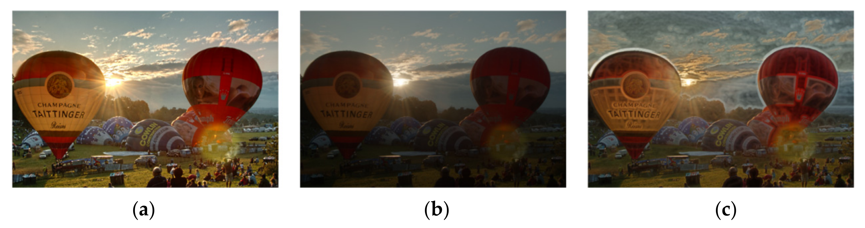
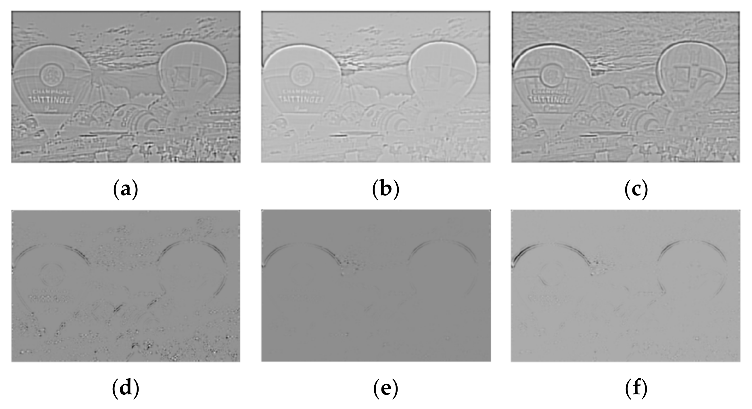
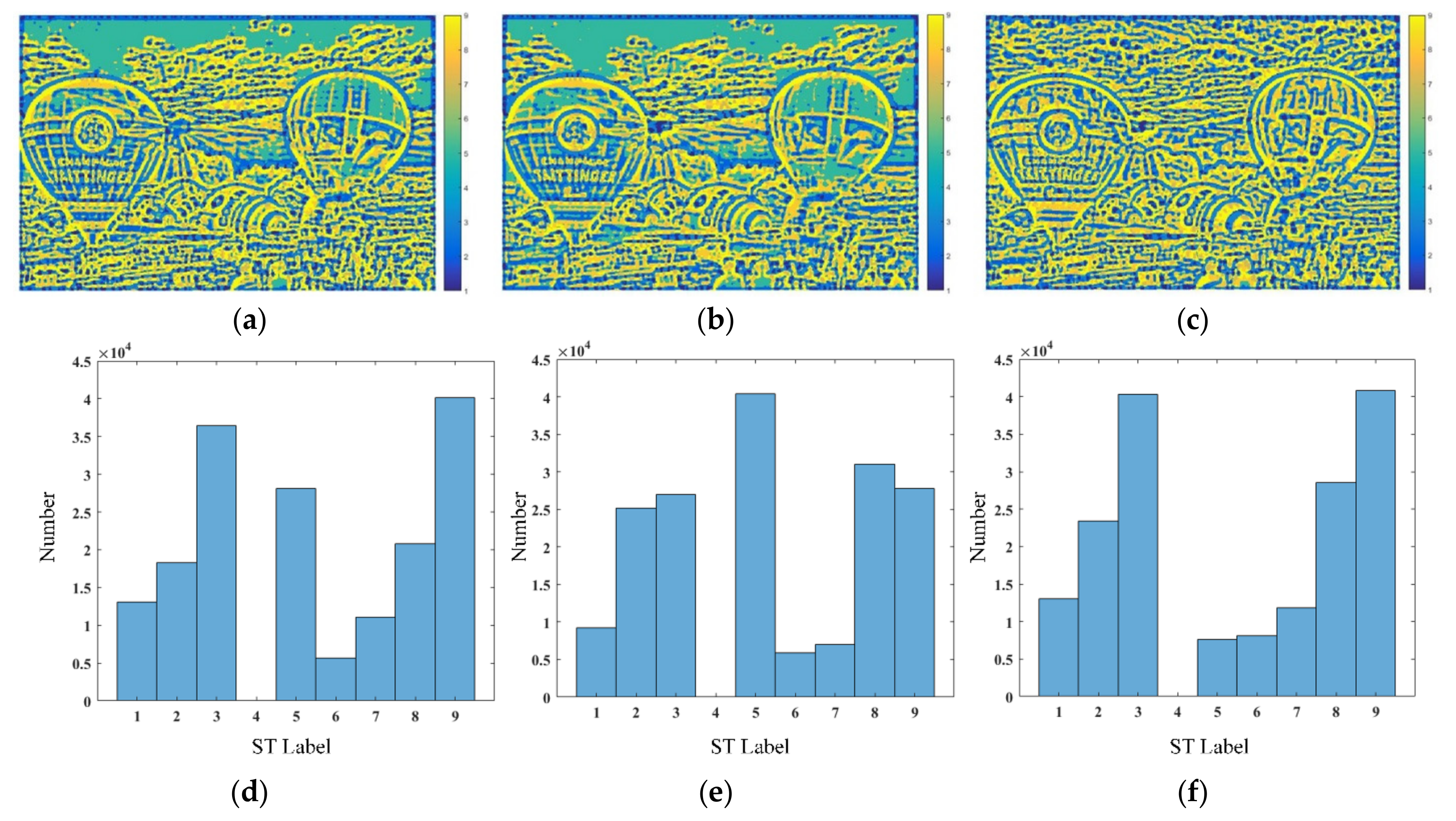
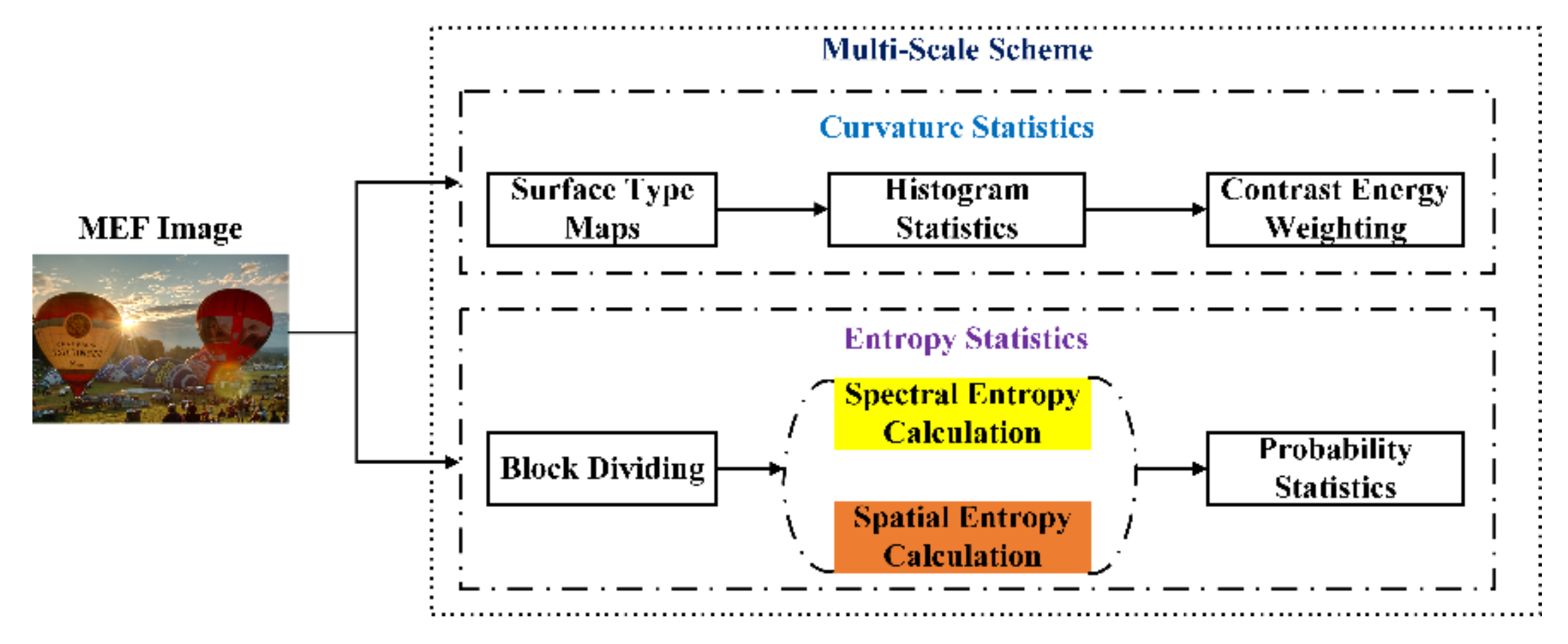
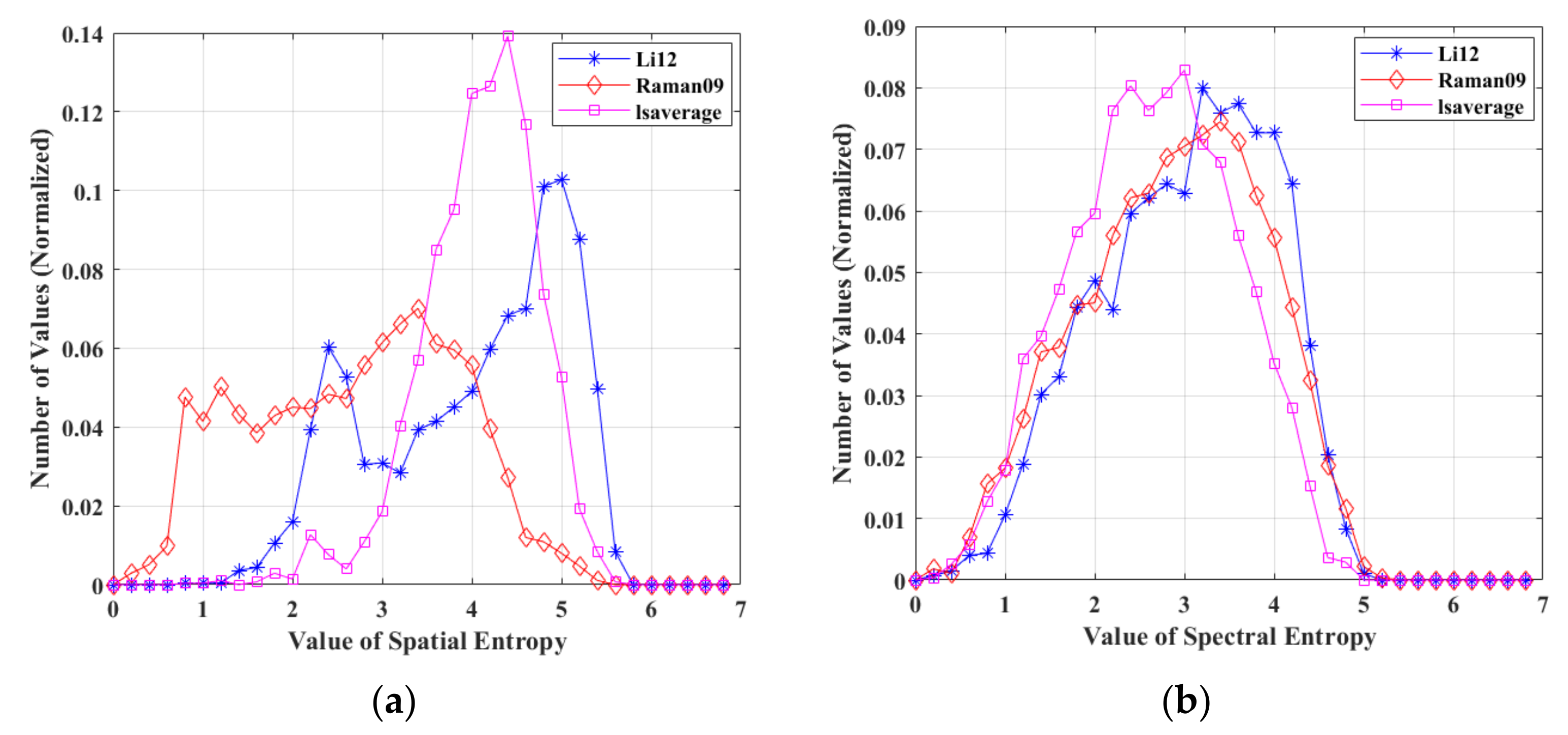
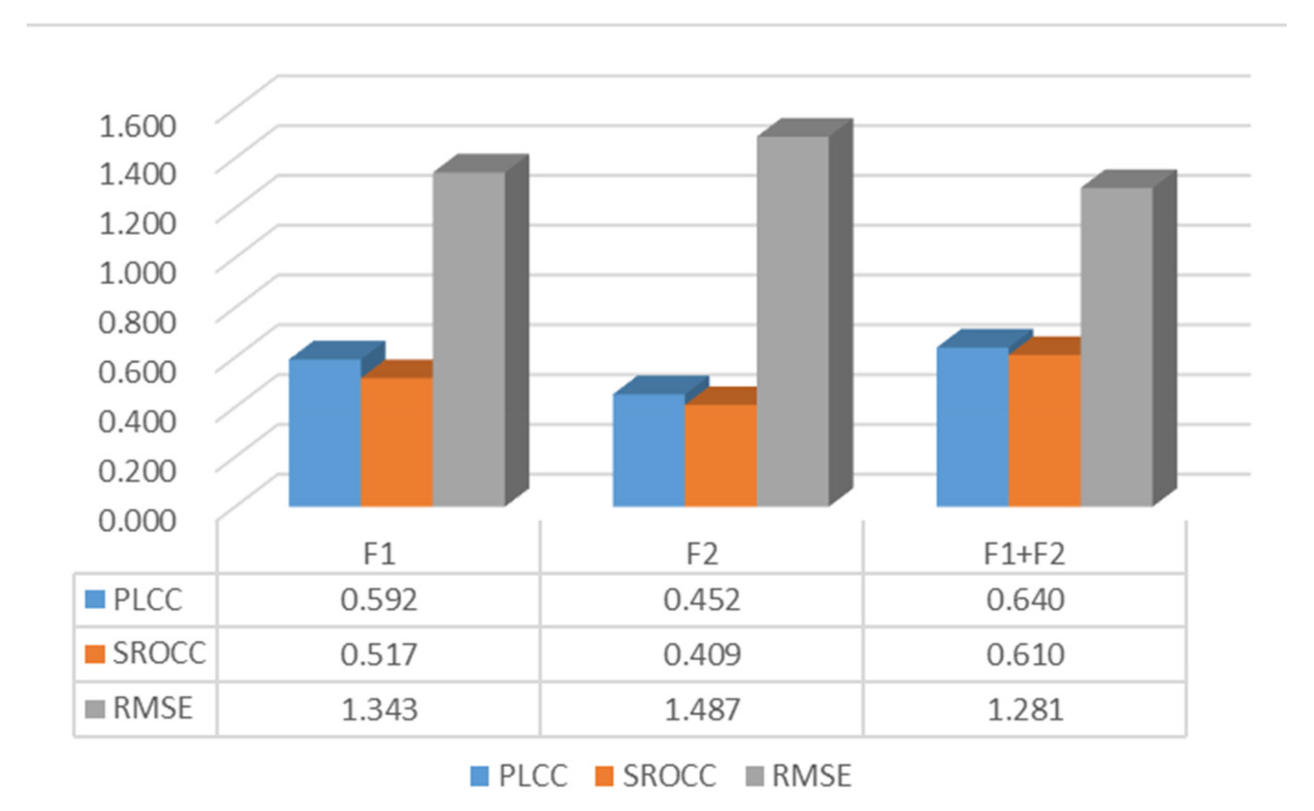
- In terms of structure and detail distortion introduced by inappropriate exposure conditions, the histogram statistics features of surface type maps generated from the mean and Gaussian curvature, and entropy statistics features in the spatial and spectral domains are extracted to form the quality-aware feature vectors.
- (2)
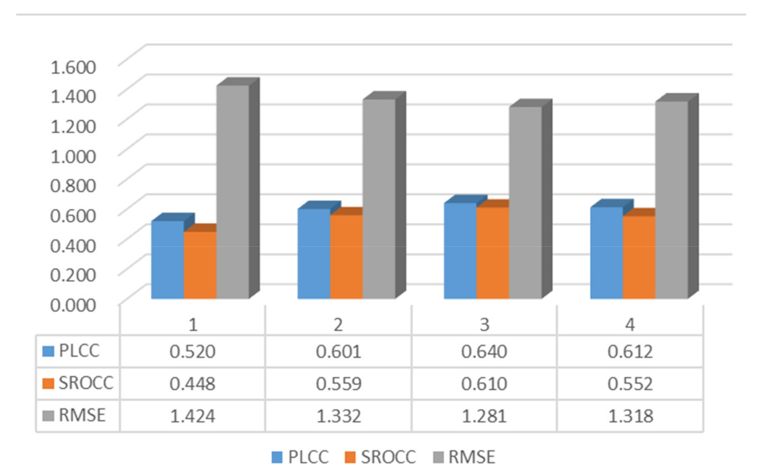
- Since the contrast variation is a key factor affecting the quality of the MEF image, contrast energy weights are designed to aggregate the above curvature features. Furthermore, a multi-scale scheme is adopted to perceive the distortion of the image in different resolutions for simulating the multi-channel characteristics in the human visual system.
- (3)
- Considering that it is significant for multimedia applications to bridge the gap between BIQA methods and MEF images, a novel CE-BMIQA method specialized for MEF images is proposed. Experimental results on the available MEF database demonstrate the superiority of the proposed CE-BMIQA method compared with the state-of-the-art BIQA methods.
2. Proposed CE-BMIQA Method
2.1. Curvature Statistics
2.2. Entropy Statistic
2.3. Quality Regression
3. Experiment Results and Analysis
3.1. Database and Experimental Protocols
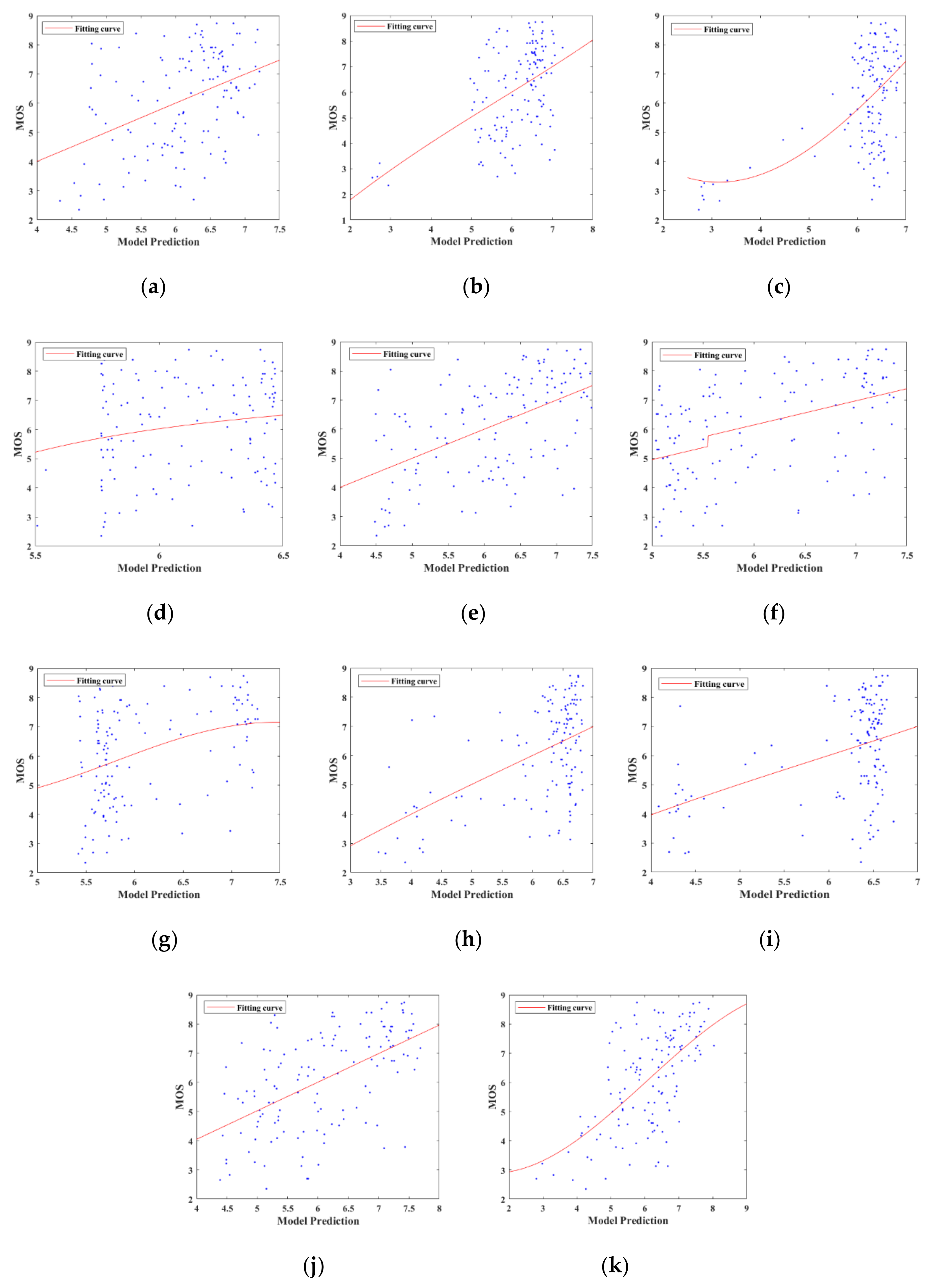
3.2. Performance Comparison
3.3. Impacts of Individual Feature Set
3.4. Impacts of Scale Number and Computational Complexity
4. Further Discussion
- (1)
- The detail loss usually occurs in the overexposure and underexposure regions of MEF images. In general, the degree of detail preservation also varies with different environmental compositions under different exposure conditions. Therefore, accurate segmentation methods for different exposure regions and semantic segmentation methods can be applied to design BIQA methods for MEF images in the future.
- (2)
- Generally, the natural scene is almost colorful and moving in practice. When the quality of the MEF image is not good, the color will inevitably be affected, so color is also one of the factors that need to be considered. In future work, color analysis will be concentrated to develop more valuable BIQA methods for MEF images.
5. Conclusions
Author Contributions
Funding
Data Availability Statement
Conflicts of Interest
References
- Kinoshita, Y.; Kiya, H. Scene segmentation-based luminance adjustment for multi-exposure image fusion. IEEE Trans. Image Process. 2019, 28, 4101–4116. [Google Scholar] [CrossRef] [Green Version]
- Qi, Y.; Zhou, S.; Zhang, Z.; Luo, S.; Lin, X.; Wang, L.; Qiang, B. Deep unsupervised learning based on color un-referenced loss functions for multi-exposure image fusion. Inf. Fusion 2021, 66, 18–39. [Google Scholar] [CrossRef]
- Ma, K.; Zeng, K.; Wang, Z. Perceptual quality assessment for multi-exposure image fusion. IEEE Trans. Image Process. 2015, 24, 3345–3356. [Google Scholar] [CrossRef]
- Wang, Z.; Bovik, A.C. Reduced and no reference visual quality assessment. IEEE Signal Process. Mag. 2011, 29, 29–40. [Google Scholar] [CrossRef]
- Mittal, A.; Moorthy, A.K.; Bovik, A.C. No-reference image quality assessment in the spatial domain. IEEE Trans. Image Process. 2012, 21, 4695–4708. [Google Scholar] [CrossRef]
- Moorthy, A.K.; Bovik, A.C. Blind image quality assessment: From natural scene statistics to perceptual quality. IEEE Trans. Image Process. 2011, 20, 3350–3364. [Google Scholar] [CrossRef]
- Saad, M.A.; Bovik, A.C.; Charrier, C. Blind image quality assessment: A natural scene statistics approach in the DCT domain. IEEE Trans. Image Process. 2012, 21, 3339–3352. [Google Scholar] [CrossRef]
- Li, Q.; Lin, W.; Fang, Y. No-reference quality assessment for multiply-distorted images in gradient domain. IEEE Signal Process. Lett. 2016, 23, 541–545. [Google Scholar] [CrossRef]
- Liu, L.; Hua, Y.; Zhao, Q.; Huang, H.; Bovik, A.C. Blind image quality assessment by relative gradient statistics and adaboosting neural network. Signal Process. Image Commun. 2016, 40, 1–15. [Google Scholar] [CrossRef]
- Oszust, M. Local feature descriptor and derivative filters for blind image quality assessment. IEEE Signal Process. Lett. 2019, 26, 322–326. [Google Scholar] [CrossRef]
- Liu, L.; Dong, H.; Huang, H.; Bovik, A.C. No-reference image quality assessment in curvelet domain. Signal Process. Image Commun. 2014, 29, 494–505. [Google Scholar] [CrossRef]
- Gu, K.; Lin, W.; Zhai, G.; Yang, X.; Zhang, W.; Chen, C.W. No-reference quality metric of contrast-distorted images based on information maximization. IEEE Trans. Cybern. 2017, 47, 4559–4565. [Google Scholar] [CrossRef]
- Rana, A.; Singh, P.; Valenzise, G.; Dufaux, F.; Komodakis, N.; Smolic, A. Deep tone mapping operator for high dynamic 397 range images. IEEE Trans. Image Process. 2019, 29, 1285–1298. [Google Scholar] [CrossRef] [Green Version]
- Gu, K.; Wang, S.; Zhai, G.; Ma, S.; Yang, X.; Lin, W.; Zhang, W.; Gao, W. Blind quality assessment of tone-mapped images via analysis of information, naturalness, and structure. IEEE Trans. Multimed. 2016, 18, 432–443. [Google Scholar] [CrossRef]
- Kundu, D.; Ghadiyaram, D.; Bovik, A.C.; Evans, B.L. No-reference quality assessment of tone-mapped HDR pictures. IEEE Trans. Image Process. 2017, 26, 2957–2971. [Google Scholar] [CrossRef]
- Xing, L.; Cai, L.; Zeng, H.G.; Chen, J.; Zhu, J.Q.; Hou, J.H. A multi-scale contrast-based image quality assessment model for multi-exposure image fusion. Signal Process. 2018, 145, 233–240. [Google Scholar] [CrossRef]
- Deng, C.W.; Li, Z.; Wang, S.G.; Liu, X.; Dai, J.H. Saturation-based quality assessment for colorful multi-exposure image fusion. Int. J. Adv. Robot. Syst. 2017, 14, 1–15. [Google Scholar] [CrossRef]
- Rahman, H.; Soundararajan, R.; Babu, R.V. Evaluating multiexposure fusion using image information. IEEE Signal Process. Lett. 2017, 24, 1671–1675. [Google Scholar] [CrossRef]
- Martinez, J.; Pistonesi, S.; Maciel, M.C.; Flesia, A.G. Multiscale fidelity measure for image fusion quality assessment. Inf. Fusion 2019, 50, 197–211. [Google Scholar] [CrossRef]
- Wang, Z.; Bovik, A.C.; Sheikh, H.R.; Simoncelli, E.P. Image quality assessment: From error visibility to structural similarity. IEEE Trans. Image Process. 2004, 13, 600–612. [Google Scholar] [CrossRef] [PubMed] [Green Version]
- Li, Z.; Zheng, J.; Rahardja, S. Detail-enhanced exposure fusion. IEEE Trans. Image Process. 2012, 21, 4672–4676. [Google Scholar] [PubMed]
- Raman, S.; Chaudhuri, S. Bilateral filter based compositing for variable exposure photography. In Proceedings of the Eurographics (Short Papers), Munich, Germany, 30 March–3 April 2009; pp. 1–3. [Google Scholar]
- Gu, B.; Li, W.; Wong, J.; Zhu, M.; Wang, M. Gradient field multi-exposure images fusion for high dynamic range image visualization. J. Vis. Commun. Image Represent. 2012, 23, 604–610. [Google Scholar] [CrossRef]
- Besl, P.J.; Jain, R.C. Segmentation through variable-order surface fitting. IEEE Trans. Pattern Anal. Mach. Intell. 1988, 10, 167–192. [Google Scholar] [CrossRef] [Green Version]
- Do Carmo, M.P. Differential Geometry of Curves and Surfaces; Prentice-Hall: Englewood Cliffs, NJ, USA, 1976. [Google Scholar]
- Choi, L.K.; You, J.; Bovik, A.C. Referenceless prediction of perceptual fog density and perceptual image defogging. IEEE Trans. Image Process. 2015, 24, 3888–3901. [Google Scholar] [CrossRef]
- Multi-exposure Fusion Image Database. Available online: http://ivc.uwaterloo.ca/database/MEF/MEFDatabase.php (accessed on 11 July 2015).
- Li, S.; Kang, X. Fast multi-exposure image fusion with median filter and recursive filter. IEEE Trans. Consum. Electron. 2012, 58, 626–632. [Google Scholar] [CrossRef] [Green Version]
- Li, S.; Kang, X.; Hu, J. Image fusion with guided filtering. IEEE Trans. Image Process. 2013, 22, 2864–2875. [Google Scholar] [PubMed]
- Mertens, T.; Kautz, J.; Van Reeth, F. Exposure fusion: A simple and practical alternative to high dynamic range photography. Comput. Graph. Forum 2009, 28, 161–171. [Google Scholar] [CrossRef]
- Antkowiak, J.; Baina, T.J. Final Report from the Video Quality Experts Group on the Validation of Objective Models of Video Quality Assessment; ITU-T Standards Contributions COM: Geneva, Switzerland, 2000. [Google Scholar]
- Groen, I.I.A.; Ghebreab, S.; Prins, H.; Lamme, V.A.F.; Scholte, H.S. From image statistics to scene gist: Evoked neural activity reveals transition from low-level natural image structure to scene category. J. Neurosci. 2013, 33, 18814–18824. [Google Scholar] [CrossRef] [PubMed] [Green Version]


| No. | Step |
|---|---|
| 1 | Input MEF images |
| 2 | Extract distortion features |
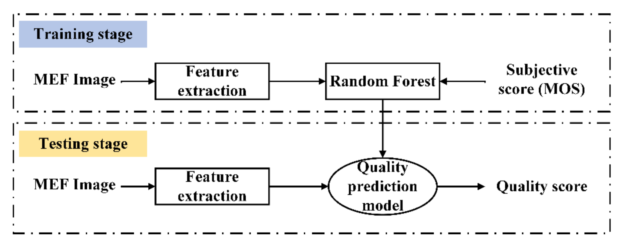
| 3 | Training stage: train a quality prediction model via random forest (which means learning a mapping relationship between feature space and subjective score). Subjective score means mean opinion score (MOS) which is provided in the subjective database. |
| 4 | Testing stage: calculate the objective quality score of a MEF image via the trained quality prediction model |
| Gc > 0 | Gc = 0 | Gc < 0 | |
|---|---|---|---|
| Mc < 0 | Peak (ST = 1) | Ridge (ST = 2) | Saddle Ridge (ST = 3) |
| Mc = 0 | None (ST = 4) | Flat (ST = 5) | Minimal (ST = 6) |
| Mc > 0 | Pit (ST = 7) | Valley (ST = 8) | Saddle Valley (ST = 9) |
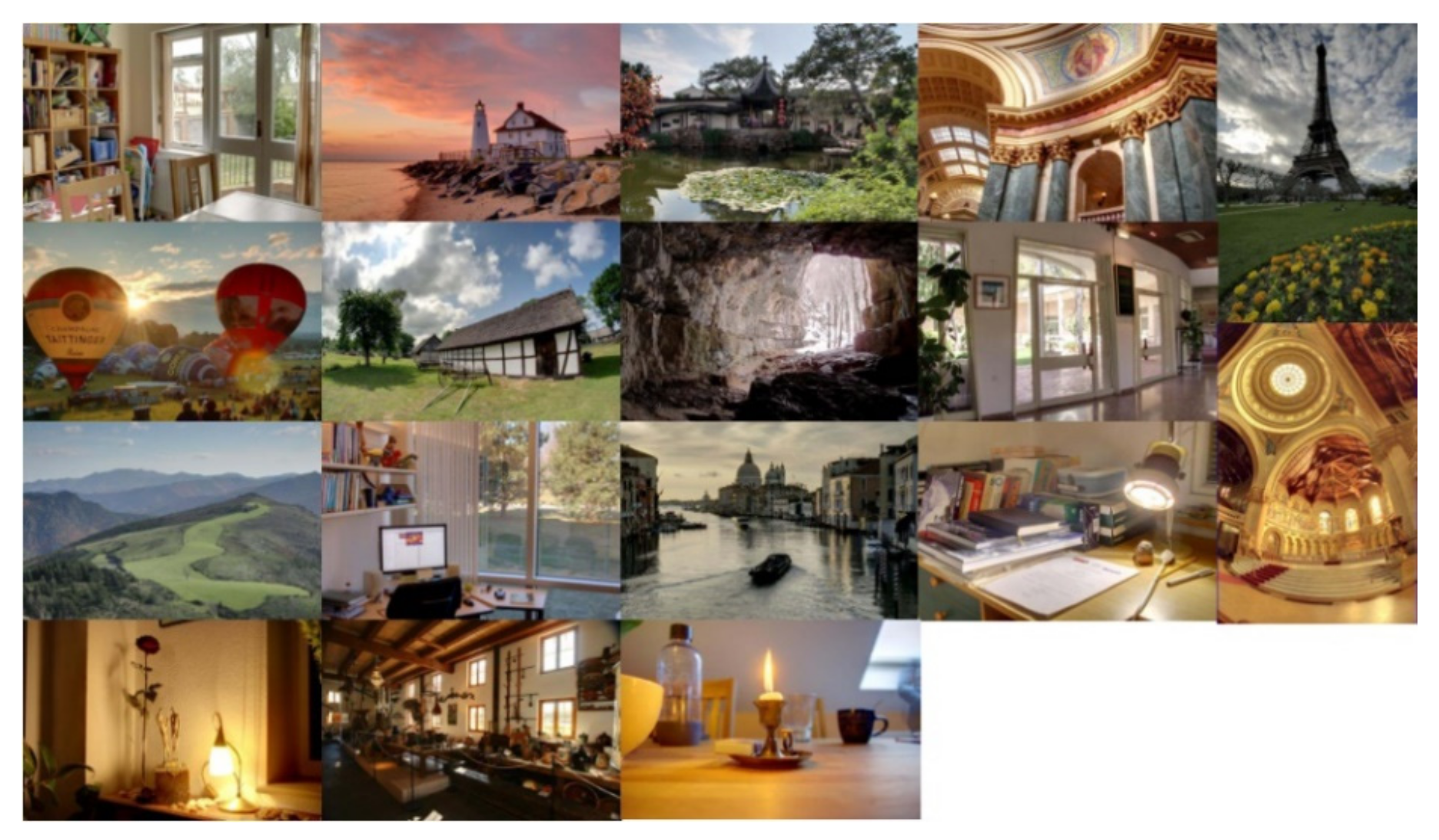
| No. | Source Sequences | Size | Image Source |
|---|---|---|---|
| 1 | Balloons | 339 × 512 × 9 | Erik Reinhard |
| 2 | Belgium house | 512 × 384 × 9 | Dani Lischinski |
| 3 | Lamp1 | 512 × 384 × 15 | Martin Cadik |
| 4 | Candle | 512 × 364 × 10 | HDR Projects |
| 5 | Cave | 512 × 384 × 4 | Bartlomiej Okonek |
| 6 | Chinese garden | 512 × 340 × 3 | Bartlomiej Okonek |
| 7 | Farmhouse | 512 × 341 × 3 | HDR Projects |
| 8 | House | 512 × 340 × 4 | Tom Mertens |
| 9 | Kluki | 512 × 341 × 3 | Bartlomiej Okonek |
| 10 | Lamp2 | 512 × 342 × 6 | HDR Projects |
| 11 | Landscape | 512 × 341 × 3 | HDRsoft |
| 12 | Lighthouse | 512 × 340 × 3 | HDRsoft |
| 13 | Madison capitol | 512 × 384 × 30 | Chaman Singh Verma |
| 14 | Memorial | 341 × 512 × 16 | Paul Debevec |
| 15 | Office | 512 × 340 × 6 | Matlab |
| 16 | Tower | 341 × 512 × 3 | Jacques Joffre |
| 17 | Venice | 512 × 341 × 3 | HDRsoft |
| No. | Methods | ||||||||||
|---|---|---|---|---|---|---|---|---|---|---|---|
| [5] | [6] | [7] | [8] | [9] | [10] | [11] | [12] | [14] | [15] | Proposed | |
| 1 | 0.916 | 0.829 | 0.774 | 0.886 | 0.945 | 0.921 | 0.672 | 0.823 | 0.883 | 0.934 | 0.578 |
| 2 | 0.877 | 0.840 | 0.703 | 0.718 | 0.799 | 0.891 | 0.851 | 0.110 | 0.677 | 0.983 | 0.851 |
| 3 | 0.886 | 0.751 | 0.848 | 0.844 | 0.791 | 0.763 | 0.817 | 0.941 | 0.341 | 0.895 | 0.923 |
| 4 | 0.825 | 0.884 | 0.876 | 0.275 | 0.548 | 0.779 | 0.043 | 0.760 | 0.974 | 0.412 | 0.880 |
| 5 | 0.130 | 0.496 | 0.658 | 0.796 | 0.619 | 0.788 | 0.191 | 0.233 | 0.522 | 0.466 | 0.538 |
| 6 | 0.008 | 0.137 | 0.344 | 0.231 | 0.898 | 0.349 | 0.644 | 0.593 | 0.086 | 0.835 | 0.995 |
| 7 | 0.729 | 0.548 | 0.460 | 0.223 | 0.923 | 0.832 | 0.856 | 0.767 | 0.841 | 0.710 | 0.848 |
| 8 | 0.662 | 0.760 | 0.556 | 0.725 | 0.591 | 0.891 | 0.983 | 0.841 | 0.890 | 0.968 | 0.967 |
| 9 | 0.792 | 0.763 | 0.850 | 0.628 | 0.803 | 0.793 | 0.406 | −0.321 | −0.120 | 0.861 | 0.882 |
| 10 | 0.718 | 0.831 | 0.902 | 0.405 | 0.781 | 0.651 | 0.897 | 0.643 | 0.543 | 0.962 | 0.045 |
| 11 | 0.816 | 0.770 | 0.862 | 0.276 | 0.778 | 0.581 | 0.588 | 0.457 | 0.667 | 0.942 | 0.948 |
| 12 | 0.937 | 0.904 | 0.871 | 0.781 | 0.938 | 0.685 | 0.994 | 0.894 | 0.647 | 0.805 | 0.995 |
| 13 | 0.642 | 0.727 | 0.516 | 0.676 | 0.758 | 0.701 | 0.939 | 0.597 | 0.750 | 0.746 | 0.941 |
| 14 | 0.667 | 0.682 | 0.955 | 0.828 | 0.461 | 0.816 | −0.935 | 0.826 | 0.475 | 0.783 | 0.978 |
| 15 | 0.856 | 0.821 | 0.856 | 0.703 | 0.834 | 0.712 | 0.868 | 0.884 | 0.025 | 0.901 | 0.923 |
| 16 | 0.761 | 0.901 | 0.526 | 0.636 | 0.935 | 0.595 | 0.699 | 0.532 | 0.666 | 0.501 | 0.705 |
| 17 | 0.990 | 0.423 | 0.852 | 0.914 | 0.840 | 0.709 | 0.866 | 0.549 | 0.240 | 0.736 | 0.837 |
| All | 0.414 | 0.491 | 0.534 | 0.163 | 0.523 | 0.481 | 0.371 | 0.519 | 0.452 | 0.561 | 0.640 |
| Hit Count | 1 | 1 | 0 | 1 | 2 | 0 | 1 | 1 | 1 | 2 | 8 |
| No. | Methods | ||||||||||
|---|---|---|---|---|---|---|---|---|---|---|---|
| [5] | [6] | [7] | [8] | [9] | [10] | [11] | [12] | [14] | [15] | Proposed | |
| 1 | 0.833 | 0.714 | 0.738 | 0.667 | 0.881 | 0.857 | 0.310 | 0.524 | 0.786 | 0.762 | 0.405 |
| 2 | 0.731 | 0.635 | 0.515 | 0.527 | 0.826 | 0.731 | 0.802 | 0.240 | 0.407 | 0.898 | 0.659 |
| 3 | 0.476 | 0.643 | 0.548 | 0.381 | 0.905 | 0.714 | 0.571 | 0.738 | 0.476 | 0.714 | 0.910 |
| 4 | 0 | 0.810 | 0.310 | −0.381 | 0.143 | 0.762 | −0.286 | 0.429 | 0.191 | 0.095 | 0.119 |
| 5 | 0.238 | 0.143 | 0.333 | 0.714 | 0.167 | 0.333 | 0.119 | 0.381 | 0.643 | 0 | 0.578 |
| 6 | 0.191 | 0.214 | 0.310 | 0.286 | 0.595 | 0.191 | 0.333 | 0.381 | 0.143 | 0.857 | 0.976 |
| 7 | 0.595 | 0.548 | 0.191 | −0.095 | 0.786 | 0.595 | 0.810 | 0.286 | 0.524 | 0.714 | 0.667 |
| 8 | 0.500 | 0.524 | 0.476 | 0.643 | 0.524 | 0.762 | 0.905 | 0.786 | 0.738 | 0.786 | 0.905 |
| 9 | 0.405 | 0.738 | 0.786 | 0.310 | 0.714 | 0.810 | 0.357 | 0.333 | 0 | 0.738 | 0.833 |
| 10 | 0.714 | 0.643 | 0.786 | −0.262 | −0.143 | 0.548 | 0.786 | 0.429 | 0.429 | 0.786 | 0.095 |
| 11 | 0.191 | 0.667 | 0.881 | 0.167 | 0.643 | 0.738 | 0.119 | −0.357 | −0.595 | 0.810 | 0.883 |
| 12 | 0.810 | 0.912 | 0.191 | 0.381 | 0.810 | 0.810 | 0.905 | 0.095 | −0.571 | 0.786 | 0.929 |
| 13 | 0.595 | 0.691 | 0.357 | 0.143 | 0.643 | 0.619 | 0.905 | 0.190 | 0.595 | 0.762 | 0.786 |
| 14 | 0.095 | 0.476 | 0.714 | −0.071 | 0.167 | 0.762 | 0.905 | 0.595 | 0.405 | 0.786 | 0.833 |
| 15 | 0.711 | 0.615 | 0.783 | 0.530 | 0.651 | 0.783 | 0.566 | 0.783 | −0.205 | 0.843 | 0.964 |
| 16 | 0.286 | 0.833 | 0.405 | −0.524 | 0.929 | 0.738 | 0.071 | 0.192 | 0.619 | 0.691 | 0.738 |
| 17 | 0.252 | −0.192 | 0.719 | 0.683 | 0.276 | 0.671 | 0.742 | 0.275 | 0.108 | 0.743 | 0.635 |
| All | 0.380 | 0.403 | 0.346 | 0.113 | 0.525 | 0.494 | 0.337 | 0.404 | 0.343 | 0.566 | 0.610 |
| Hit Count | 0 | 1 | 1 | 1 | 2 | 0 | 5 | 0 | 0 | 3 | 8 |
| Metrics | BRISQUE | DIIVINE | BLINDS-II | GWH-GLBP | OG-IQA | SCORER |
| Time (sec.) | 0.041 | 6.602 | 14.736 | 0.058 | 0.031 | 0.588 |
| Metrics | CurveletQA | NIQMC | BTMQI | HIGRADE | Proposed | |
| Time (sec.) | 2.5141 | 1.9241 | 0.076 | 0.260 | 0.480 |
Publisher’s Note: MDPI stays neutral with regard to jurisdictional claims in published maps and institutional affiliations. |
© 2021 by the authors. Licensee MDPI, Basel, Switzerland. This article is an open access article distributed under the terms and conditions of the Creative Commons Attribution (CC BY) license (https://creativecommons.org/licenses/by/4.0/).
Share and Cite
He, Z.; Song, Y.; Zhong, C.; Li, L. Curvature and Entropy Statistics-Based Blind Multi-Exposure Fusion Image Quality Assessment. Symmetry 2021, 13, 1446. https://doi.org/10.3390/sym13081446
He Z, Song Y, Zhong C, Li L. Curvature and Entropy Statistics-Based Blind Multi-Exposure Fusion Image Quality Assessment. Symmetry. 2021; 13(8):1446. https://doi.org/10.3390/sym13081446
Chicago/Turabian StyleHe, Zhouyan, Yang Song, Caiming Zhong, and Li Li. 2021. "Curvature and Entropy Statistics-Based Blind Multi-Exposure Fusion Image Quality Assessment" Symmetry 13, no. 8: 1446. https://doi.org/10.3390/sym13081446
APA StyleHe, Z., Song, Y., Zhong, C., & Li, L. (2021). Curvature and Entropy Statistics-Based Blind Multi-Exposure Fusion Image Quality Assessment. Symmetry, 13(8), 1446. https://doi.org/10.3390/sym13081446