
A Descriptor-Based Advanced Feature Detector for Improved Visual Tracking


Abstract
:1. Introduction
2. Related Work
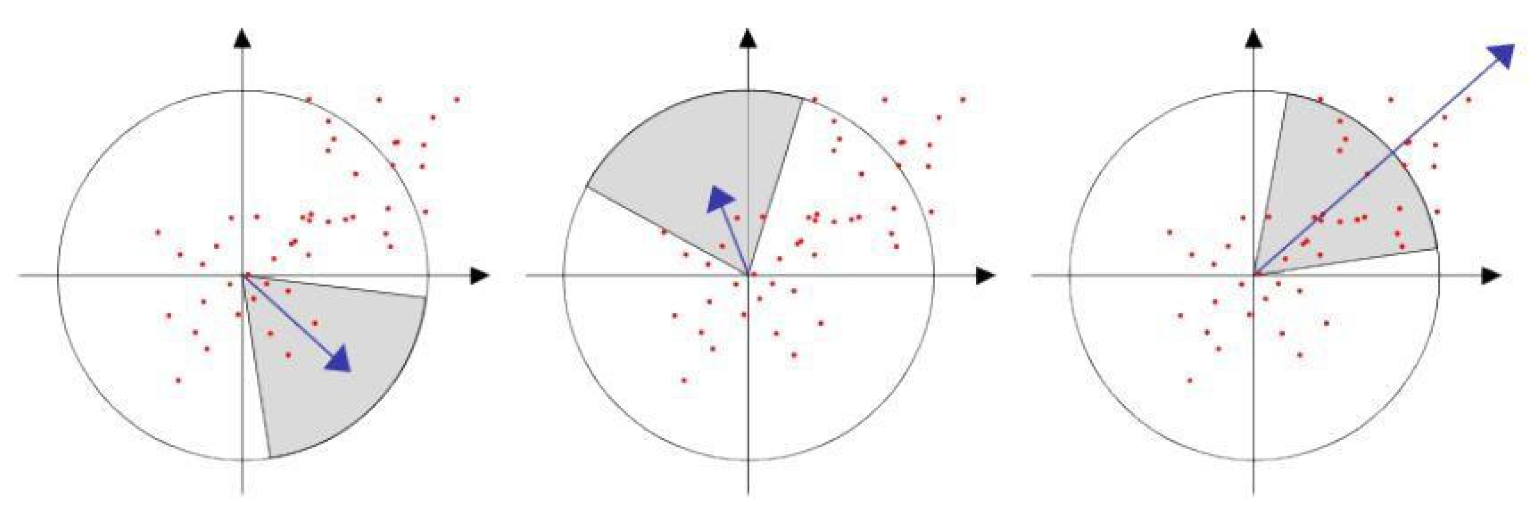
2.1. SURF
2.2. MSER
2.3. Harris Detector
2.4. Minimum Eigenvalue Detector
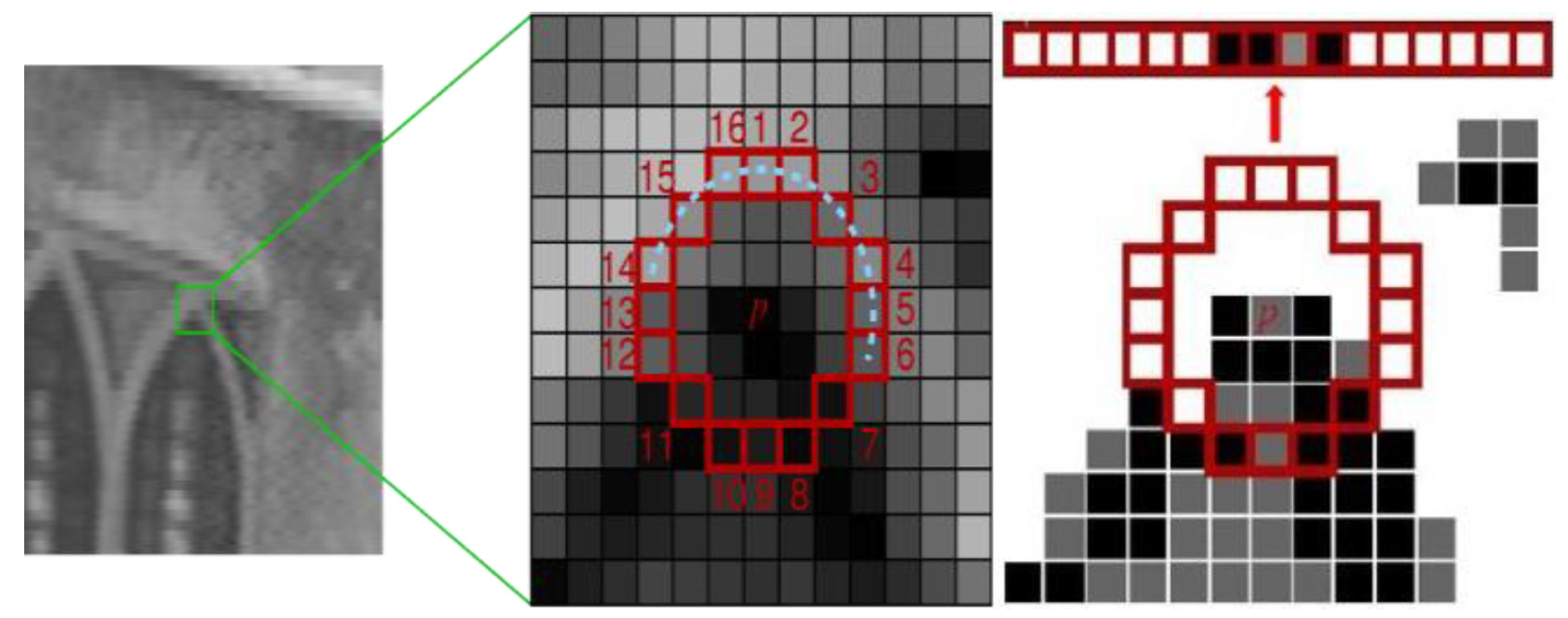
2.5. FAST
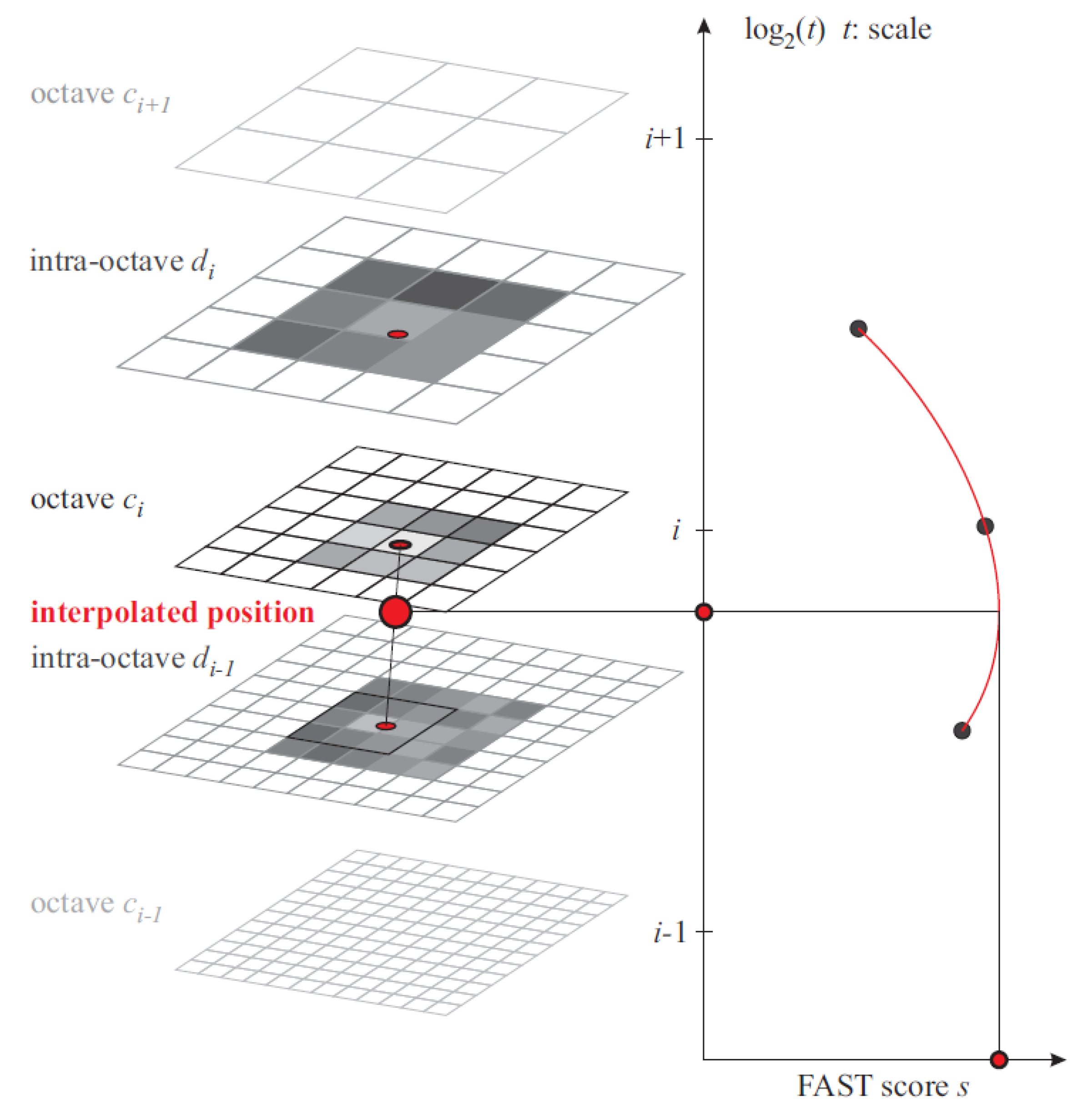
2.6. BRISK
2.7. FREAK
3. Proposed Algorithm
3.1. Feature Points Detection
- Conversion to grayscale. The SRF algorithm only works with a 2D image grayscale matrix, and any image format must be converted into a grayscale matrix format before proceeding to the next step. In this analysis, the grayscale conversion is done through the MATLAB built-in function, whereby the RGB to grayscale conversion is done using Equation (4):
- Reduction of image resolution. This step aims to decrease the computational cost of the algorithm without affecting the output significantly. Thus, this step is not necessary if there is no restriction on the computational cost. In this stage, the image resolution is reduced to half by removing the even rows and columns. This kind of subsampling will not affect the performance of finding feature points, especially for those large images. Then, the image resolution is decreased to half again by combining four adjacent pixels into one and obtaining the average value. This process can decrease the computational load and image noise simultaneously with the drawback of the blurring effect.
- Calculation of the gradient intensity. This is used by the Harris detector, whereby the gradient intensity of every pixel is estimated in the x-direction, y-direction, and xy-direction using the convolution method with a mask matrix of [−1 0 1] shown in Equation (5):
- Obtaining feature points. Only the points with large gradient intensity are selected as feature points. The average value from the three gradient intensities is measured with second-order derivatives (, , ), and the threshold is set according to the highest average gradient intensity value to ensure consistent performance regardless of the light intensity of the image, as shown in Equations (6) and (7):
- Filtering the feature points. Feature points within the same region should at least connect one adjacent point using the SRF algorithm. If the number of connected feature points is too small, it is assumed that these feature points are image noise and should be eliminated.
3.2. Features Description
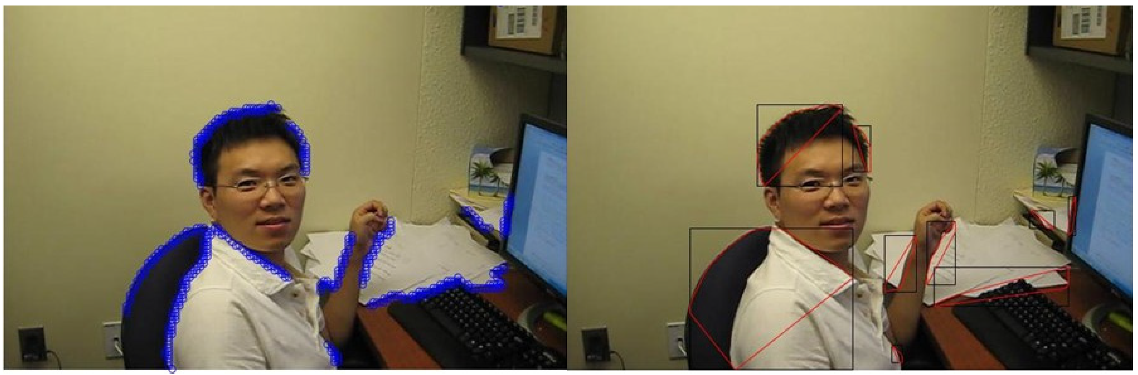
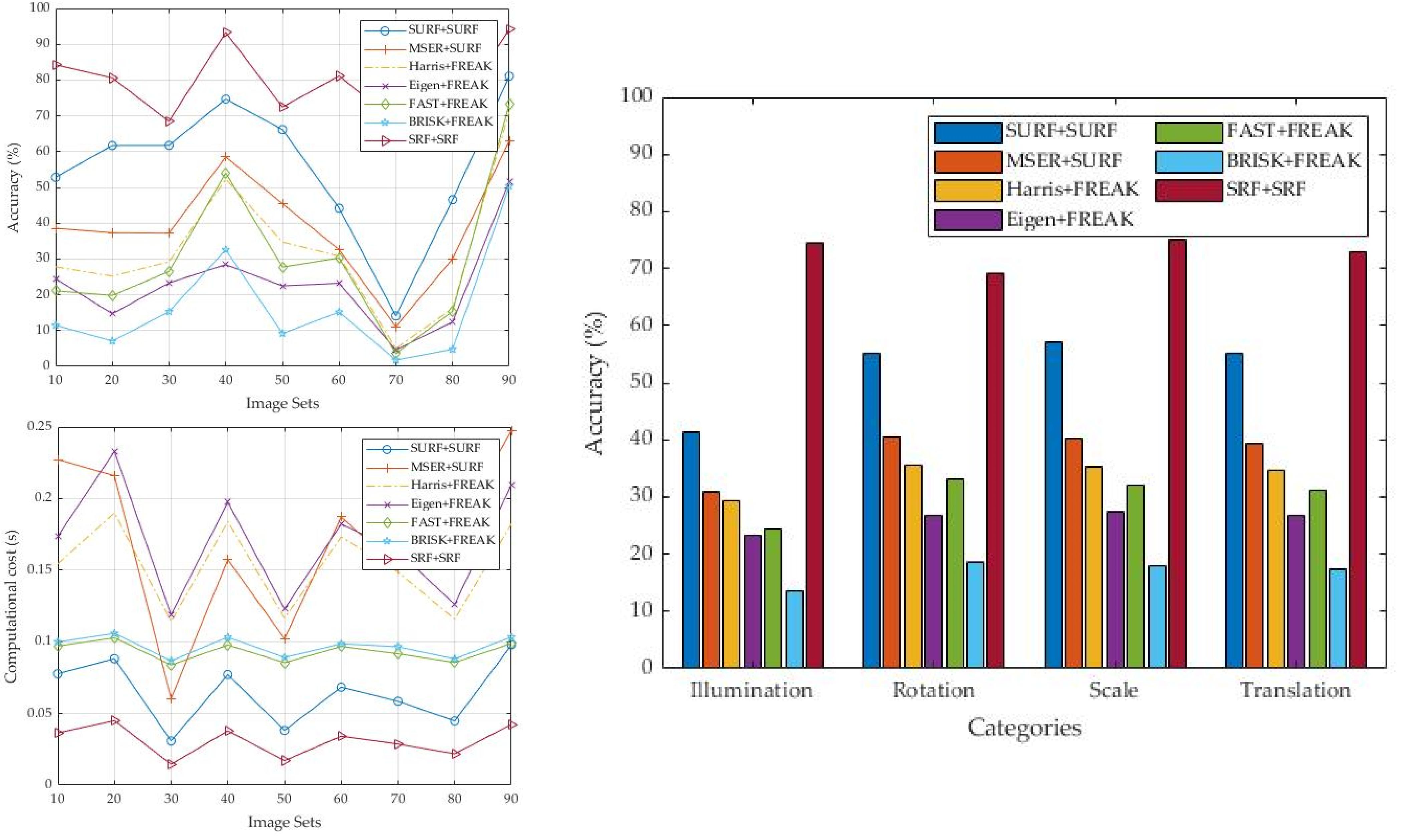
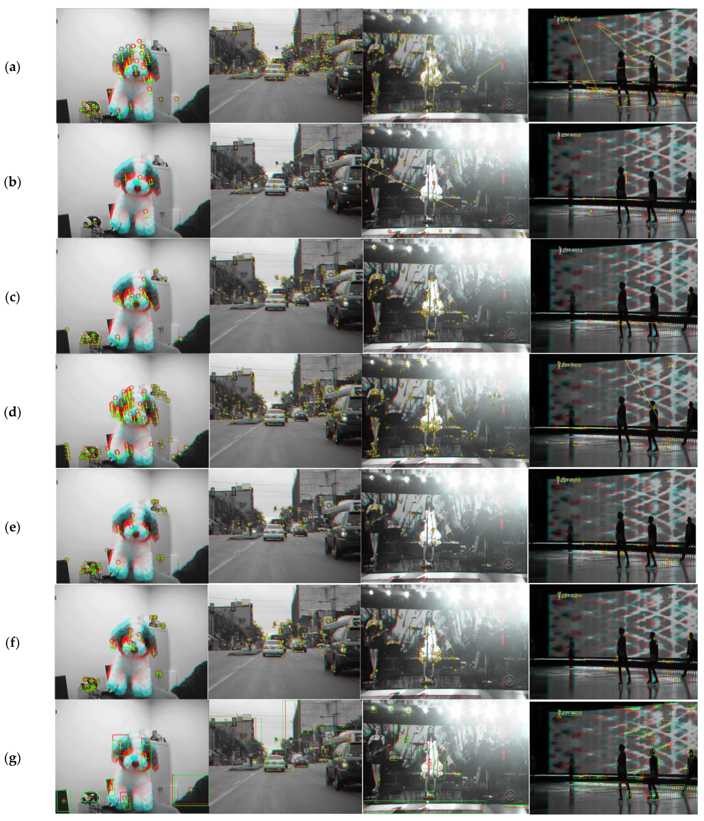
3.3. Performance Evaluation
4. Results and Discussions
5. Conclusions
Author Contributions
Funding
Institutional Review Board Statement
Informed Consent Statement
Data Availability Statement
Acknowledgments
Conflicts of Interest
References
- Thakur, N.; Han, C. An Ambient Intelligence-Based Human Behavior Monitoring Framework for Ubiquitous Environments. Information 2021, 12, 81. [Google Scholar] [CrossRef]
- Mouats, T.; Aouf, N.; Nam, D.; Vidas, S. Performance Evaluation of Feature Detectors and Descriptors Beyond the Visible. J. Intell. Robot. Syst. 2018, 92, 33–63. [Google Scholar] [CrossRef] [Green Version]
- Alahi, A.; Ortiz, R.; VanderGheynst, P. FREAK: Fast Retina Keypoint. In Proceedings of the 2012 IEEE Conference on Computer Vision and Pattern Recognition, Providence, RI, USA, 16–21 June 2012; pp. 510–517. [Google Scholar]
- Zhu, Y.; Tong, M.; Jiang, Z.; Zhong, S.; Tian, Q. Hybrid feature-based analysis of video’s affective content using protagonist detection. Expert Syst. Appl. 2019, 128, 316–326. [Google Scholar] [CrossRef]
- Leutenegger, S.; Chli, M.; Siegwart, R.Y. BRISK: Binary robust invariant scalable keypoints. Proceedings of Computer Vision (ICCV), Barcelona, Spain, 6–13 November 2011; pp. 2548–2555. [Google Scholar]
- Varytimidis, C.; Rapantzikos, K.; Avrithis, Y.; Kollias, S. α-shapes for local feature detection. Pattern Recognit. 2016, 50, 56–73. [Google Scholar] [CrossRef] [Green Version]
- Lee, M.H.; Cho, M.; Park, I.K. Feature description using local neighborhoods. Pattern Recognit. Lett. 2015, 68, 76–82. [Google Scholar] [CrossRef]
- Wang, Y.; Fan, J.; Qian, C.; Guo, L. Ego-motion estimation using sparse SURF flow in monocular vision systems. Int. J. Adv. Robot. Syst. 2016, 13, 1729881416671112. [Google Scholar] [CrossRef] [Green Version]
- Kang, T.-K.; Choi, I.-H.; Lim, M.-T. MDGHM-SURF: A robust local image descriptor based on modified discrete Gaussian–Hermite moment. Pattern Recognit. 2015, 48, 670–684. [Google Scholar] [CrossRef]
- Nistér, D.; Stewénius, H. Linear Time Maximally Stable Extremal Regions. In Proceedings of the Transactions on Petri Nets and Other Models of Concurrency XV; Springer Science and Business Media LLC: Berlin/Heidelberg, Germany, 2008; pp. 183–196. [Google Scholar]
- Obdržálek, D.; Basovník, S.; Mach, L.; Mikulík, A. Detecting Scene Elements Using Maximally Stable Colour Regions. In Proceedings of the Communications in Computer and Information Science; Springer Science and Business Media LLC: Berlin/Heidelberg, Germany, 2010; pp. 107–115. [Google Scholar]
- Harris, C.; Stephens, M. A combined corner and edge detector. In Proceedings of the Alvey Vision Conference, Manchester, UK, 31 August–2 September 1988; Volume 15, pp. 147–151. [Google Scholar]
- Parks, D.; Gravel, J.-P. Corner detection. Int. J. Comput. Vision 2004, 1–17. [Google Scholar]
- Shi, J.; Tomasi, C. Good Features to Track. In Proceedings of the IEEE Conference on Computer Vision and Pattern Recognition, Seattle, DC, USA, 21–23 June 1994; pp. 593–600. [Google Scholar]
- Rosten, E.; Drummond, T. Machine Learning for High-Speed Corner Detection. In Proceedings of the Transactions on Petri Nets and Other Models of Concurrency XV; Springer Science and Business Media LLC: Berlin/Heidelberg, Germany, 2006; pp. 430–443. [Google Scholar]
- Işık, Ş. A Comparative Evaluation of Well-known Feature Detectors and Descriptors. Int. J. Appl. Math. Electron. Comput. 2014, 3, 1–6. [Google Scholar] [CrossRef] [Green Version]
- Loncomilla, P.; Ruiz-Del-Solar, J.; Martínez, L. Object recognition using local invariant features for robotic applications: A survey. Pattern Recognit. 2016, 60, 499–514. [Google Scholar] [CrossRef]
- Wu, Y.; Su, Q.; Ma, W.; Liu, S.; Miao, Q. Learning Robust Feature Descriptor for Image Registration with Genetic Programming. IEEE Access 2020, 8, 39389–39402. [Google Scholar] [CrossRef]
- Jurgensen, S.M. The Rotated Speeded-Up Robust Features Algorithm (R-SURF); Naval Postgraduate School: Monterey, CA, USA, 2014. [Google Scholar]
- Chen, L.-C.; Hsieh, J.-W.; Yan, Y.; Chen, D.-Y. Vehicle make and model recognition using sparse representation and symmetrical SURFs. Pattern Recognit. 2015, 48, 1979–1998. [Google Scholar] [CrossRef]
- Matas, J.; Chum, O.; Urban, M.; Pajdla, T. Robust wide-baseline stereo from maximally stable extremal regions. Image Vis. Comput. 2004, 22, 761–767. [Google Scholar] [CrossRef]
- Bok, Y.; Ha, H.; Kweon, I.S. Automated checkerboard detection and indexing using circular boundaries. Pattern Recognit. Lett. 2016, 71, 66–72. [Google Scholar] [CrossRef]
- Přibyl, B.; Chalmers, A.; Zemčík, P.; Hooberman, L.; Čadík, M. Evaluation of feature point detection in high dynamic range imagery. J. Vis. Commun. Image Represent. 2016, 38, 141–160. [Google Scholar] [CrossRef]
- Elfakiri, Y.; Khaissidi, G.; Mrabti, M.; Chenouni, D.; El Yacoubi, M. Word spotting for handwritten Arabic documents using Harris detector. In Proceedings of the 2016 International Conference on Information Technology for Organizations Development (IT4OD), Fez, Morocco, 30 March–1 April 2016; pp. 1–4. [Google Scholar]
- Orguner, U.; Gustafsson, F. Statistical Characteristics of Harris Corner Detector. In Proceedings of the 2007 IEEE/SP 14th Workshop on Statistical Signal Processing, Madison, WI, USA, 26–29 August 2007; pp. 571–575. [Google Scholar]
- Hassaballah, M.; Abdelmgeid, A.A.; Alshazly, H.A. Image Features Detection, Description and Matching. In Econometrics for Financial Applications; Springer Science and Business Media LLC: Berlin/Heidelberg, Germany, 2016; pp. 11–45. [Google Scholar]
- Rosten, E.; Porter, R.; Drummond, T. Faster and Better: A Machine Learning Approach to Corner Detection. IEEE Trans. Pattern Anal. Mach. Intell. 2010, 32, 105–119. [Google Scholar] [CrossRef] [Green Version]
- Sharif, H.; Hölzel, M. A comparison of prefilters in ORB-based object detection. Pattern Recognit. Lett. 2017, 93, 154–161. [Google Scholar] [CrossRef]
- Fularz, M.; Kraft, M.; Schmidt, A.; Kasiński, A. A High-Performance FPGA-Based Image Feature Detector and Matcher Based on the FAST and BRIEF Algorithms. Int. J. Adv. Robot. Syst. 2015, 12, 141. [Google Scholar] [CrossRef] [Green Version]
- Persson, A.; Loutfi, A. Fast Matching of Binary Descriptors for Large-Scale Applications in Robot Vision. Int. J. Adv. Robot. Syst. 2016, 13, 58. [Google Scholar] [CrossRef] [Green Version]
- Garway-Heath, D.F.; Caprioli, J.; Fitzke, F.W.; Hitchings, R. Scaling the hill of vision: The physiological relationship between light sensitivity and ganglion cell numbers. Investig. Ophthalmol. Vis. Sci. 2000, 41, 1774–1782. [Google Scholar]
- Ester, M.; Kriegel, H.P.; Sander, J.; Xu, X. Density-based spatial clustering of applications with noise. Int. Conf. Knowl. Discov. Data Min. 1996, 240, 6. [Google Scholar]
- Yuan, C.; Yang, H. Research on K-Value Selection Method of K-Means Clustering Algorithm. J 2019, 2, 226–235. [Google Scholar] [CrossRef] [Green Version]
- Liu, J.; Bu, F. Improved RANSAC features image-matching method based on SURF. J. Eng. 2019, 2019, 9118–9122. [Google Scholar] [CrossRef]
- Setiawan, A.; Yunmar, R.A.; Tantriawan, H. Comparison of Speeded-Up Robust Feature (SURF) and Oriented FAST and Rotated BRIEF (ORB) Methods in Identifying Museum Objects Using Low Light Intensity Images; IOP Conference Series: Earth and Environmental Science; IOP Publishing: South Lampung, Indonesia, 2020; Volume 537, No. 1; p. 012025. [Google Scholar]
- Wu, Y.; Lim, J.; Yang, M.-H. Online Object Tracking: A Benchmark. In Proceedings of the 2013 IEEE Conference on Computer Vision and Pattern Recognition, Portland, OR, USA, 23–28 June 2013; pp. 2411–2418. [Google Scholar]
- Luo, M.; Zhou, B.; Wang, T. Multi-part and scale adaptive visual tracker based on kernel correlation filter. PLoS ONE 2020, 15, e0231087. [Google Scholar] [CrossRef] [PubMed] [Green Version]


| Algorithm | Accuracy (%) | ||||||
|---|---|---|---|---|---|---|---|
| 1st Set | 2nd Set | 3rd Set | … | 97th Set | 98th Set | Average | |
| SURF | 60.7 | 83.1 | 32.9 | … | 87.2 | 63.8 | 55.4 |
| MSER | 40.1 | 65.8 | 27.0 | … | 82.8 | 47.7 | 39.6 |
| Harris | 28.9 | 75.9 | 12.0 | … | 85.8 | 53.8 | 34.7 |
| Eigen | 24.1 | 66.7 | 9.5 | … | 85.3 | 42.2 | 26.7 |
| FAST | 22.9 | 71.5 | 9.8 | … | 87.8 | 48.1 | 31.3 |
| BRISK | 7.0 | 48.8 | 5.2 | … | 80.1 | 26.6 | 17.4 |
| SRF | 64.4 | 95.5 | 73.2 | … | 93.0 | 82.1 | 73.1 |
| Algorithm. | Computational Cost (s) | ||||||
|---|---|---|---|---|---|---|---|
| 1st Set | 2nd Set | 3rd Set | … | 97th Set | 98th Set | Average | |
| SURF | 0.03 | 0.04 | 0.06 | … | 0.08 | 0.11 | 0.06 |
| MSER | 0.07 | 0.10 | 0.11 | … | 0.22 | 0.36 | 0.14 |
| Harris | 0.11 | 0.11 | 0.15 | … | 0.17 | 0.16 | 0.14 |
| Eigen | 0.11 | 0.11 | 0.15 | … | 0.25 | 0.19 | 0.16 |
| FAST | 0.08 | 0.08 | 0.09 | … | 0.10 | 0.10 | 0.09 |
| BRISK | 0.08 | 0.09 | 0.10 | … | 0.10 | 0.10 | 0.09 |
| SRF | 0.01 | 0.02 | 0.02 | … | 0.04 | 0.05 | 0.03 |
Publisher’s Note: MDPI stays neutral with regard to jurisdictional claims in published maps and institutional affiliations. |
© 2021 by the authors. Licensee MDPI, Basel, Switzerland. This article is an open access article distributed under the terms and conditions of the Creative Commons Attribution (CC BY) license (https://creativecommons.org/licenses/by/4.0/).
Share and Cite
Kok, K.Y.; Rajendran, P. A Descriptor-Based Advanced Feature Detector for Improved Visual Tracking. Symmetry 2021, 13, 1337. https://doi.org/10.3390/sym13081337
Kok KY, Rajendran P. A Descriptor-Based Advanced Feature Detector for Improved Visual Tracking. Symmetry. 2021; 13(8):1337. https://doi.org/10.3390/sym13081337
Chicago/Turabian StyleKok, Kai Yit, and Parvathy Rajendran. 2021. "A Descriptor-Based Advanced Feature Detector for Improved Visual Tracking" Symmetry 13, no. 8: 1337. https://doi.org/10.3390/sym13081337
APA StyleKok, K. Y., & Rajendran, P. (2021). A Descriptor-Based Advanced Feature Detector for Improved Visual Tracking. Symmetry, 13(8), 1337. https://doi.org/10.3390/sym13081337