Newton’s Third Law in the Framework of Special Relativity for Charged Bodies

Abstract

Newton’s third law states that any action is countered by a reaction of equal magnitude but opposite direction. The total force in a system not affected by external forces is, therefore, zero. However, according to the principles of relativity, a signal cannot propagate at speeds exceeding the speed of light. Hence, the action and reaction cannot be generated at the same time due to the relativity of simultaneity. Thus, the total force cannot be null at a given time. In a previous paper, we showed that Newton’s third law cannot strictly hold in a distributed system where the different parts are at a finite distance from each other. This analysis led to the suggestion of a relativistic engine. As the system is affected by a total force for a finite period, the system acquires mechanical momentum and energy. The subject of momentum conversation was discussed in another previous paper, while energy conservation was discussed in additional previous papers. In those works, we relied on the fact that the bodies were macroscopically natural. Here, we relax this assumption and study charged bodies, thus analyzing the consequences on a possible electric relativistic engine.

1. Introduction

Special relativity is a theory of the structure of space-time. It was introduced in Einstein’s famous 1905 paper, “On the Electrodynamics of Moving Bodies” [1]. This theory was a consequence of empiric observations and the laws of electromagnetism, which were formulated in the middle of the nineteenth century by Maxwell in his famous four partial differential equations [2,3,4] which owe their current form to Oliver Heaviside [5]. One of the consequences of these equations is that an electromagnetic signal travels at the speed of light c, which led people to believe that light is an electromagnetic wave. This was later used by Albert Einstein [1,3,4] to formulate his special theory of relativity, which postulates that the speed of light in vacuum c is the maximal allowed velocity in nature. According to the theory of relativity, any object, message, signal (even if not electromagnetic), or field cannot travel faster than the speed of light in vacuum, hence retardation: if someone at a distance R from an observer changes something, the observer will not know about it for at least a retardation time of $\frac{R}{c}$. This means that action and its reaction cannot be generated simultaneously because of the signal finite propagation speed.

Newton’s laws of motion are three physical laws that, together, laid the foundation for classical mechanics. These laws describe the relationship between the body, acting forces, and motion of body in response to those forces. The three laws of motion were first compiled by Isaac Newton in his Philosophiae Naturalis Principia Mathematica (Mathematical Principles of Natural Philosophy), first published in 1687 [6,7]. In this paper, we are interested only in the third law, which states the following: when one body exerts a force on a second body, the second body simultaneously exerts a force equal in magnitude and opposite in direction on the first body.

According to Newton’s third law, the total sum of forces in a system which is not affected by external forces is null. This law has a great number of experimental verification and is thus one of the corner stones of physical sciences. However, it is easy to see that action and its reaction cannot be generated at exactly the same time because the speed of signal propagation is not infinite. Hence, the third law cannot be correct in an exact sense, although it can be assumed to be valid for most practical applications due to the high velocity of signal propagation. Thus, the total sum of forces cannot be zero at every given time.

Current locomotive systems are based on coupled material parts; each gains momentum that is equal and opposite to the momentum obtained by the other. A generic example is a rocket that sheds gas to move itself forward. However, relativistic effects suggest a different type of motor that is not composed of two material elements but of matter and field. Ignoring the field, it seems that the material body obtains momentum, thus the total momentum grows, violating momentum conservation. However, it can be shown that the opposite amount of momentum is attributed to the field [8], thus the total momentum is indeed conserved. This is a result of Noether’s theorem, which dictates that a system that possesses translational symmetry will conserve momentum. The total physical system composed of matter and field is indeed invariant under translations, while every part of the system (either matter or field) is not. Feynman [4] describes two orthogonally moving charges, apparently contradicting Newton’s third law, as the forces that the charges induce do not cancel (last part of 26-2); this is resolved in 27-6 in which it is noticed that the momentum gained by the two-charge system is lost to the field.

A relativistic engine is thus defined as a system in which its material center of mass is in motion, due to the interaction of its material components. Those parts may move with respect to each other or be held in a rigid frame. This does not matter, as we are interested in the motion of the center of mass. We underline that a relativistic motor allows three-axis motion (vertical included). It does not contain moving parts and it does not consume fuel (and does not emit carbon); it only consumes electromagnetic energy which may be supplied by solar panels. The relativistic engine is perfect for space travel in which much of the space vehicle volume is devoted to fuel storage.

In the current paper, we assume that the medium’s magnetization and polarization are negligible, and therefore we do not consider corrections to the Lorentz force suggested by [9]. Griffiths and Heald [10] pointed out that the laws of Coulomb and Biot–Savart determine the electric and magnetic field configurations solely for static sources. Time-dependent generalizations of these laws described by Jefimenko [11,12] were used to study the applicability of Coulomb and Biot–Savart formulas outside the static domain.

In an earlier paper, we made use of Jefimenko’s [3,11] equation to study the force developing between two current loops [13]. This was later generalized to include the forces between a current carrying loop and a permanent magnet [14,15]. Since the device is forced for a finite period, the device will posses mechanical momentum and energy. The question then arises whether we need to abandon the law of momentum and energy conservation. The subject of momentum conversation was discussed in [8]. In [16,17,18,19], the exchange of energy between the mechanical part of the relativistic engine and the electromagnetic field were discussed. In particular, it was shown that the total electromagnetic energy expenditure is six times the kinetic energy gained by the relativistic motor. It was also shown that some energy might be radiated from the relativistic engine device if the coils are not configured properly.

The previous analysis relied on the fact that the bodies were macroscopically natural, which means that the number of electrons and ions is equal in every volume element. Here, we relax this assumption and study charged bodies, thus analyzing the consequences of charge on a possible electric relativistic engine.

We shall consider two cases; in the first, we assume an instantaneous action at a distance, in which Newton’s third law is satisfied, and the total force is equal to zero. Next, we consider the time-dependent case where the reaction to an action cannot occur before having the action-generated information reaches the affected body, thus causing a non-zero resultant. We stress that the bodies themselves are taken to be stationary; it is only the charge densities in them that are modified with time.

We highlight the main contributions of the current paper as follows:

• Although the fact that Newton’s third law is not generally respected for electromagnetic interacting systems is known [4,13], there is no published formula for the force or the momentum that can be achieved for such a charged system. This deficiency is amended in the current paper.
• It is found that in a charged system, one may achieve higher forces and momenta with respect to an uncharged system by many orders of magnitude.
• We study some possible implementations of a charged relativistic engine, and discuss the engine limitations, which are due to the phenomena of dielectric breakdown and the maximal amount of current density that one can transfer through a wire, even if superconducting.
• We suggest a way to overcome those limitations that takes advantage of the high-charge densities that are available in microscopic structures, such as ionic crystals.

2. The Electro-Static Condition

Consider two bodies having volume elements $d^3{x}_1,d^3{x}_2$ located at ${\overrightarrow{x}}_1,{\overrightarrow{x}}_2$ respectively and having static charge densities ${\rho }_1,{\rho }_2$ (see Figure 1).

The electro-static force applied by charged body 2 on charged body 1 is given by Jackson [3]:

$${\overrightarrow{F}}_{12}=\frac{1}{4\pi {ϵ}_0}\int \int \frac{d^3{x}_1{d}^3{x}_2{\rho }_1\left({\overrightarrow{x}}_1\right){\rho }_2\left({\overrightarrow{x}}_2\right){\overrightarrow{x}}_{12}}{|{\overrightarrow{x}}_{12}{|}^3}.$$

(1)

where, ${\overrightarrow{x}}_{12}={\overrightarrow{x}}_1-{\overrightarrow{x}}_2$ and ${ϵ}_0=8.85{10}^{-12}$${\mathrm{Fm}}^{-1}$ is the vacuum permittivity. From the above, it is easy to calculate the electro-static force applied by current loop 1 on charged body 2 by changing indices $1\leftrightarrow 2$:

$${\overrightarrow{F}}_{21}=\frac{1}{4\pi {ϵ}_0}\int \int \frac{d^3{x}_1{d}^3{x}_2{\rho }_1\left({\overrightarrow{x}}_1\right){\rho }_2\left({\overrightarrow{x}}_2\right){\overrightarrow{x}}_{21}}{|{\overrightarrow{x}}_{12}{|}^3}.$$

(2)

However,

$${\overrightarrow{x}}_{21}={\overrightarrow{x}}_2-{\overrightarrow{x}}_1=-({\overrightarrow{x}}_1-{\overrightarrow{x}}_2)=-{\overrightarrow{x}}_{12},|{\overrightarrow{x}}_{21}|=|{\overrightarrow{x}}_{12}|$$

(3)

We obtain the following:

$${\overrightarrow{F}}_{21}=-{\overrightarrow{F}}_{12}.$$

(4)

In addition, the total force on the two charged systems is null:

$${\overrightarrow{F}}_T={\overrightarrow{F}}_{12}+{\overrightarrow{F}}_{21}=0.$$

(5)

The above result is independent of the geometry of the charged bodies and is in complete agreement with Newton’s third law.

3. The Dynamic Electromagnetic Condition

Consider the generic time-dependent case. According to Maxwell’s equations, one does not have a magnetic field without the presence of an electric field and vice versa. We thus consider both the electric and magnetic components of Lorentz force ${\overrightarrow{F}}_{21}$. The electric field $\overrightarrow{E}$ and magnetic field $\overrightarrow{B}$ are created by charged entity 1 and act upon a charged body 2. A charged body may contain ions and free electrons, so we obtain the Lorentz force as follows:

$${\overrightarrow{F}}_{21}=\int d^3{x}_2{\rho }_{i2}(\overrightarrow{E}+{\overrightarrow{v}}_{i2}\times \overrightarrow{B})+\int d^3{x}_2{\rho }_{e2}(\overrightarrow{E}+{\overrightarrow{v}}_{e2}\times \overrightarrow{B}).$$

(6)

In the above, we integrate over the entire volume of charged body 2. ${\rho }_{i2}$ and ${\rho }_{e2}$ are the ion charge density and electron charge density, respectively. ${\overrightarrow{v}}_{i2}$ and ${\overrightarrow{v}}_{e2}$ are the ion velocity field and electron velocity field, respectively. The total charge density amounts the sum of the ions charge density and free electrons charge density, hence the following:

$${\rho }_2={\rho }_{i2}+{\rho }_{e2}.$$

(7)

Thus, the electric terms in the above force equation cancel and we are left with the following:

$${\overrightarrow{F}}_{21}=\int d^3{x}_2{\rho }_2\overrightarrow{E}+\int d^3{x}_2{\rho }_{i2}{\overrightarrow{v}}_{i2}\times \overrightarrow{B}+\int d^3{x}_2{\rho }_{e2}{\overrightarrow{v}}_{e2}\times \overrightarrow{B}.$$

(8)

In the laboratory frame, with the ions being at rest, we have the following: ${\overrightarrow{v}}_{i2}=0$. Thus, we arrive at the following:

$${\overrightarrow{F}}_{21}=\int d^3{x}_2{\rho }_2\overrightarrow{E}+\int d^3{x}_2{\rho }_{e2}{\overrightarrow{v}}_{e2}\times \overrightarrow{B}.$$

(9)

Introducing the current density: ${\overrightarrow{J}}_2={\rho }_{e2}{\overrightarrow{v}}_{e2}$, we obtain the following:

$${\overrightarrow{F}}_{21}=\int d^3{x}_2\left({\rho }_2\overrightarrow{E}+{\overrightarrow{J}}_2\times \overrightarrow{B}\right).$$

(10)

Now, let us consider the coil that generates the magnetic field. The electric and magnetic fields can be written as follows in terms of the vector and scalar potentials [3]:

$$\overrightarrow{E}=-{\partial }_t\overrightarrow{A}-\overrightarrow{\nabla }\mathsf{\Phi }.$$

(11)

$$\overrightarrow{B}=\overrightarrow{\nabla }\times \overrightarrow{A}.$$

(12)

Here, $\overrightarrow{\nabla }$ has the standard definition in vector analysis, t is time and ${\partial }_t$ is a partial derivative with respect to time. If the field is generated by a charge density ${\rho }_1$ and current density ${\overrightarrow{J}}_1$ in charged body 1, we can solve for the scalar and vector potentials and obtain the following result [3]:

$$\mathsf{\Phi }\left({\overrightarrow{x}}_2\right)=\frac{1}{4\pi {ϵ}_0}\int d^3{x}_1\frac{{\rho }_1({\overrightarrow{x}}_1,t_{ret})}{R},\overrightarrow{R}\equiv {\overrightarrow{x}}_{12},t_{ret}\equiv t-\frac{R}{c}.$$

(13)

$$\overrightarrow{A}\left({\overrightarrow{x}}_2\right)=\frac{{\mu }_0}{4\pi }\int d^3{x}_1\frac{{\overrightarrow{J}}_1({\overrightarrow{x}}_1,t_{ret})}{R}.$$

(14)

Here, $c=\frac{1}{\sqrt{{ϵ}_0{\mu }_0}}$ is the speed of light in vacuum. The above solutions satisfy the Lorentz gauge conditions:

$$\overrightarrow{\nabla }·\overrightarrow{A}+\frac{1}{c^2}{\partial }_t\mathsf{\Phi }=0$$

(15)

Due to the following conservation of charge:

$$\overrightarrow{\nabla }·\overrightarrow{J}+{\partial }_t\rho =0$$

(16)

(See Appendix A). Combining Equation (14) with Equation (12), we arrive at the result:

$$\overrightarrow{B}\left({\overrightarrow{x}}_2\right)={\overrightarrow{\nabla }}_{{\overrightarrow{x}}_2}\times \overrightarrow{A}\left({\overrightarrow{x}}_2\right)=\frac{{\mu }_0}{4\pi }\int d^3{x}_1{\overrightarrow{\nabla }}_{{\overrightarrow{x}}_2}\times \left(\frac{{\overrightarrow{J}}_1({\overrightarrow{x}}_1,t_{ret})}{R}\right).$$

(17)

However, notice the following (we use the notation ${\partial }_y\equiv \frac{\partial }{\partial y}$.):

$${\overrightarrow{\nabla }}_{{\overrightarrow{x}}_2}\times \left(\frac{{\overrightarrow{J}}_1({\overrightarrow{x}}_1,t_{ret})}{R}\right)={\overrightarrow{\nabla }}_{{\overrightarrow{x}}_2}R\times {\partial }_R\left(\frac{{\overrightarrow{J}}_1({\overrightarrow{x}}_1,t_{ret})}{R}\right).$$

(18)

Since

$${\overrightarrow{\nabla }}_{{\overrightarrow{x}}_2}R=-\frac{\overrightarrow{R}}{R}$$

(19)

additionally,

$${\partial }_R\left(\frac{{\overrightarrow{J}}_1({\overrightarrow{x}}_1,t_{ret})}{R}\right)=-\frac{{\overrightarrow{J}}_1({\overrightarrow{x}}_1,t_{ret})}{R^2}-\frac{{\partial }_t{\overrightarrow{J}}_1({\overrightarrow{x}}_1,t_{ret})}{Rc}.$$

(20)

Hence,

$${\overrightarrow{\nabla }}_{{\overrightarrow{x}}_2}\times \left(\frac{{\overrightarrow{J}}_1({\overrightarrow{x}}_1,t_{ret})}{R}\right)=\frac{\overrightarrow{R}}{R^3}\times \left({\overrightarrow{J}}_1({\overrightarrow{x}}_1,t_{ret})+\left(\frac{R}{c}\right){\partial }_t{\overrightarrow{J}}_1({\overrightarrow{x}}_1,t_{ret})\right).$$

(21)

Inserting Equation (21) into Equation (17), we arrive at Jefimenko’s equations [3,11] for the magnetic field:

$$\overrightarrow{B}\left({\overrightarrow{x}}_2\right)=\frac{{\mu }_0}{4\pi }\int d^3{x}_1\frac{\overrightarrow{R}}{R^3}\times \left({\overrightarrow{J}}_1({\overrightarrow{x}}_1,t_{ret})+\left(\frac{R}{c}\right){\partial }_t{\overrightarrow{J}}_1({\overrightarrow{x}}_1,t_{ret})\right).$$

(22)

For the electric field, we have two contributions according to Equation (11), one from the scalar potential and a second one from the vector potential:

$$\overrightarrow{E}={\overrightarrow{E}}_a+{\overrightarrow{E}}_b,{\overrightarrow{E}}_a\equiv -{\partial }_t\overrightarrow{A},{\overrightarrow{E}}_b\equiv -\overrightarrow{\nabla }\mathsf{\Phi }.$$

(23)

Hence, according to Equation (14),

$${\overrightarrow{E}}_a\left({\overrightarrow{x}}_2\right)=-\frac{{\mu }_0}{4\pi }\int d^3{x}_1\frac{{\partial }_t{\overrightarrow{J}}_1({\overrightarrow{x}}_1,t_{ret})}{R}.$$

(24)

According to Equation (13),

$${\overrightarrow{E}}_b\left({\overrightarrow{x}}_2\right)=-k\int d^3{x}_1{\overrightarrow{\nabla }}_{{\overrightarrow{x}}_2}\left(\frac{{\rho }_1({\overrightarrow{x}}_1,t_{ret})}{R}\right),k\equiv \frac{1}{4\pi {ϵ}_0}\simeq 9·{10}^9.$$

(25)

The above equation can also be written as follows:

$${\overrightarrow{E}}_b\left({\overrightarrow{x}}_2\right)=-k\int d^3{x}_1\left[\frac{1}{R}{\overrightarrow{\nabla }}_{{\overrightarrow{x}}_2}{\rho }_1({\overrightarrow{x}}_1,t_{ret})+{\rho }_1({\overrightarrow{x}}_1,t_{ret}){\overrightarrow{\nabla }}_{{\overrightarrow{x}}_2}\frac{1}{R}\right],$$

(26)

however,

$${\overrightarrow{\nabla }}_{{\overrightarrow{x}}_2}\frac{1}{R}=\frac{\widehat{R}}{R^2},\widehat{R}\equiv \frac{\overrightarrow{R}}{R}$$

(27)

in addition:

$${\overrightarrow{\nabla }}_{{\overrightarrow{x}}_2}{\rho }_1({\overrightarrow{x}}_1,t_{ret})={\overrightarrow{\nabla }}_{{\overrightarrow{x}}_2}R{\left.{\partial }_R{\rho }_1({\overrightarrow{x}}_1,t_{ret})\right|}_{{\overrightarrow{x}}_1}=\frac{\widehat{R}}{c}{\partial }_t{\rho }_1({\overrightarrow{x}}_1,t_{ret}).$$

(28)

It thus follows that

$${\overrightarrow{E}}_b\left({\overrightarrow{x}}_2\right)=-k\int d^3{x}_1\frac{\widehat{R}}{R^2}\left[{\rho }_1({\overrightarrow{x}}_1,t_{ret})+\left(\frac{R}{c}\right){\partial }_t{\rho }_1({\overrightarrow{x}}_1,t_{ret})\right].$$

(29)

Adding ${\overrightarrow{E}}_b$ and ${\overrightarrow{E}}_a$ and taking into account the following,

$$\frac{{\mu }_0}{4\pi k}={\mu }_0{ϵ}_0=\frac{1}{c^2}$$

(30)

we arrive at the Jefimenko’s expression [3,11] for the electric field as follows:

$$\begin{array}{ccc}\hfill \overrightarrow{E}\left({\overrightarrow{x}}_2\right)& =& -k\int d^3{x}_1\frac{1}{R^2}\left[\left({\rho }_1({\overrightarrow{x}}_1,t_{ret})+\left(\frac{R}{c}\right){\partial }_t{\rho }_1({\overrightarrow{x}}_1,t_{ret})\right)\widehat{R}\right.\hfill \\ & +& \left.{\left(\frac{R}{c}\right)}^2\frac{{\partial }_t{\overrightarrow{J}}_1({\overrightarrow{x}}_1,t_{ret})}{R}\right].\hfill \end{array}$$

(31)

Inserting Equation (22) and Equation (31) into Equation (10), we arrive at a somewhat lengthy but straightforward expression:

$$\begin{array}{ccc}\hfill {\overrightarrow{F}}_{21}& =& -k\int \int d^3{x}_1{d}^3{x}_2\frac{1}{R^2}\hfill \\ & & \left\{{\rho }_2({\overrightarrow{x}}_2,t)\left[\left({\rho }_1({\overrightarrow{x}}_1,t_{ret})+\left(\frac{R}{c}\right){\partial }_t{\rho }_1({\overrightarrow{x}}_1,t_{ret})\right)\widehat{R}+{\left(\frac{R}{c}\right)}^2\frac{{\partial }_t{\overrightarrow{J}}_1({\overrightarrow{x}}_1,t_{ret})}{R}\right]\right.\hfill \\ & & \left.+{\left(\frac{R}{c}\right)}^2\left[\frac{\widehat{R}}{R^2}\times \left({\overrightarrow{J}}_1({\overrightarrow{x}}_1,t_{ret})+\left(\frac{R}{c}\right){\partial }_t{\overrightarrow{J}}_1({\overrightarrow{x}}_1,t_{ret})\right)\right]\times {\overrightarrow{J}}_2({\overrightarrow{x}}_2,t)\right\}\hfill \end{array}$$

(32)

3.1. The Quasi-Static Approximation

In the quasi-static approximation, it is assumed that $\tau =\frac{R}{c}$ is small and can be neglected. Under the same approximation $t_{ret}\simeq t$, neglecting all terms of order $\tau$, Equation (32) takes the following Coulomb form:

$${\overrightarrow{F}}_{21}=-k\int \int d^3{x}_1{d}^3{x}_2{\rho }_1({\overrightarrow{x}}_1,t){\rho }_2({\overrightarrow{x}}_2,t)\frac{\widehat{R}}{R^2}.$$

(33)

The above equation is similar to the Equation (2) with slightly different notation, but now the charge densities are time dependent and therefore, not static. Newton’s third law follows trivially, using the same arguments as in Section 2. We notice that for vanishing charge densities, Equation (32) takes the following form:

$$\begin{array}{ccc}\hfill {\overrightarrow{F}}_{21}& =& -k\int \int d^3{x}_1{d}^3{x}_2\frac{1}{R^2}\hfill \\ & & \left\{{\left(\frac{R}{c}\right)}^2\left[\frac{\widehat{R}}{R^2}\times \left({\overrightarrow{J}}_1({\overrightarrow{x}}_1,t_{ret})+\left(\frac{R}{c}\right){\partial }_t{\overrightarrow{J}}_1({\overrightarrow{x}}_1,t_{ret})\right)\right]\times {\overrightarrow{J}}_2({\overrightarrow{x}}_2,t)\right\}.\hfill \end{array}$$

(34)

In this case, the leading term is $O\left({\tau }^2\right)$, neglecting higher order terms in $\tau$. This can be written as follows:

$${\overrightarrow{F}}_{21}=\frac{{\mu }_0}{4\pi }\int \int d^3{x}_1{d}^3{x}_2\left\{{\overrightarrow{J}}_2({\overrightarrow{x}}_2,t)\times \left[\frac{\widehat{R}}{R^2}\times {\overrightarrow{J}}_1({\overrightarrow{x}}_1,t)\right]\right\}.$$

(35)

or as follows:

$$\begin{array}{ccc}\hfill {\overrightarrow{F}}_{21}& =& \frac{{\mu }_0}{4\pi }\int \int d^3{x}_1{d}^3{x}_2\left\{\left({\overrightarrow{J}}_2({\overrightarrow{x}}_2,t)·{\overrightarrow{J}}_1({\overrightarrow{x}}_1,t)\right)\frac{\widehat{R}}{R^2}\right.\hfill \\ & -& \left.\left({\overrightarrow{J}}_2({\overrightarrow{x}}_2,t)·\frac{\widehat{R}}{R^2}\right){\overrightarrow{J}}_1({\overrightarrow{x}}_1,t)\right\}.\hfill \end{array}$$

(36)

Notice that according to Equation (27),

$${\overrightarrow{J}}_2({\overrightarrow{x}}_2,t)·\frac{\widehat{R}}{R^2}={\overrightarrow{J}}_2({\overrightarrow{x}}_2,t)·{\overrightarrow{\nabla }}_{{\overrightarrow{x}}_2}\frac{1}{R}={\overrightarrow{\nabla }}_{{\overrightarrow{x}}_2}·\left(\frac{{\overrightarrow{J}}_2({\overrightarrow{x}}_2,t)}{R}\right)-\frac{1}{R}{\overrightarrow{\nabla }}_{{\overrightarrow{x}}_2}·{\overrightarrow{J}}_2({\overrightarrow{x}}_2,t).$$

(37)

However, since we assume that the charge density is null, it follows from Equation (16) that ${\overrightarrow{\nabla }}_{{\overrightarrow{x}}_2}·{\overrightarrow{J}}_2=0$, and

$${\overrightarrow{J}}_2({\overrightarrow{x}}_2,t)·\frac{\widehat{R}}{R^2}={\overrightarrow{\nabla }}_{{\overrightarrow{x}}_2}·\left(\frac{{\overrightarrow{J}}_2({\overrightarrow{x}}_2,t)}{R}\right).$$

(38)

Taking the volume integral of the left hand side and using Gauss theorem, we obtain the following:

$$\int d^3{x}_2{\overrightarrow{J}}_2({\overrightarrow{x}}_2,t)·\frac{\widehat{R}}{R^2}=\oint d{\overrightarrow{S}}_2·\left(\frac{{\overrightarrow{J}}_2({\overrightarrow{x}}_2,t)}{R}\right),$$

(39)

where $d{\overrightarrow{S}}_2$ and the integral is taken over the entire surface encapsulating the volume. If the surface is taken far from the system in which the current density is non-vanishing, it follows that the surface integral is null and thus,

$$\int d^3{x}_2{\overrightarrow{J}}_2({\overrightarrow{x}}_2,t)·\frac{\widehat{R}}{R^2}=0.$$

(40)

Thus, Equation (36) will take the following form:

$${\overrightarrow{F}}_{21}=\frac{{\mu }_0}{4\pi }\int \int d^3{x}_1{d}^3{x}_2\left({\overrightarrow{J}}_2({\overrightarrow{x}}_2,t)·{\overrightarrow{J}}_1({\overrightarrow{x}}_1,t)\right)\frac{\widehat{R}}{R^2}.$$

(41)

from which Newton’s third law follows trivially. We notice that this form is a generalization of a similar result presented in [13] for the case of currents that are restricted to flow on thin current loops. In the quasi-static approximation, Newton’s third law holds regardless of the geometry of the system involved, and the total force is null.

The reader should not be surprised by this result since in the quasi-static approximation, we neglect the duration that it takes a signal to propagate from part 1 to part 2, making the assumption that this time is null. Significantly different results may be obtained in the case that $\tau$ is taken into account, as we demonstrate in the next subsection.

3.2. The Case of a Finite $\tau$

Considering the charge density $\rho ({\overrightarrow{x}}^{\prime },t_{ret})=\rho ({\overrightarrow{x}}^{\prime },t-\frac{R}{c})$, if $\frac{R}{c}$ is small but not zero, one can write a Taylor series expansion around t in the following form:

$$\rho ({\overrightarrow{x}}^{\prime },t_{ret})=\rho ({\overrightarrow{x}}^{\prime },t-\frac{R}{c})=\sum _{n=0}^{\infty }\frac{{\partial }_t^n\rho ({\overrightarrow{x}}^{\prime },t)}{n!}{(-\frac{R}{c})}^n.$$

(42)

In the above, ${\partial }_t^n\rho ({\overrightarrow{x}}^{\prime },t)$ is the partial temporal derivative of order n of $\rho ({\overrightarrow{x}}^{\prime },t)$. The same expansion for the current density leads to the following expression:

$$\overrightarrow{J}({\overrightarrow{x}}^{\prime },t_{ret})=\overrightarrow{J}({\overrightarrow{x}}^{\prime },t-\frac{R}{c})=\sum _{n=0}^{\infty }\frac{{\partial }_t^n\overrightarrow{J}({\overrightarrow{x}}^{\prime },t)}{n!}{(-\frac{R}{c})}^n.$$

(43)

In the above, ${\partial }_t^n\overrightarrow{J}({\overrightarrow{x}}^{\prime },t)$ is the partial temporal derivative of order n of $\overrightarrow{J}({\overrightarrow{x}}^{\prime },t)$. The above expansions are valid only for a certain environment of t on the time axis, which depends on the functions involved; this environment shall be defined using the convergence radius $T_{max}$, which may be different for each function, that is, Equation (42) and Equation (43) are valid only in the domain $[t-T_{max},t+T_{max}]$. As we expand in the delay time $\frac{R}{c}$, it follows that the expansion is valid only for a limited range:

$$R<R_{max}\equiv c{T}_{max}.$$

(44)

This means that basically, we are dealing with a near field approximation; however, as c is a large number, $R_{max}$ would be quite large for most systems. Now, inserting Equation (42) into Equation (13) we obtain the following:

$$\begin{array}{ccc}\hfill {\mathsf{\Phi }}_1\left({\overrightarrow{x}}_2\right)& =& k\int d^3{x}_1\frac{{\rho }_1\left(t_{ret}\right)}{R}=k\sum _{n=0}^{\infty }\frac{1}{n!}\int d^3{x}_1{\partial }_t^n{\rho }_1({\overrightarrow{x}}^{\prime },t)\frac{1}{R}{(-\frac{R}{c})}^n\hfill \\ & =& k\sum _{n=0}^{\infty }\frac{1}{n!}{\left(-\frac{1}{c}\right)}^n\int d^3{x}_1{\partial }_t^n{\rho }_1({\overrightarrow{x}}_1,t)R^{n-1}\hfill \end{array}$$

(45)

Similarly, inserting Equation (43) into Equation (14), we obtain the following:

$$\begin{array}{ccc}\hfill {\overrightarrow{A}}_1\left({\overrightarrow{x}}_2\right)& =& \frac{{\mu }_0}{4\pi }\int d^3{x}_1\frac{{\overrightarrow{J}}_1\left(t_{ret}\right)}{R}=\frac{{\mu }_0}{4\pi }\sum _{n=0}^{\infty }\frac{1}{n!}\int d^3{x}_1{\partial }_t^n{\overrightarrow{J}}_1({\overrightarrow{x}}^{\prime },t)\frac{1}{R}{(-\frac{R}{c})}^n\hfill \\ & =& \frac{{\mu }_0}{4\pi }\sum _{n=0}^{\infty }\frac{1}{n!}{\left(-\frac{1}{c}\right)}^n\int d^3{x}_1{\partial }_t^n{\overrightarrow{J}}_1({\overrightarrow{x}}_1,t)R^{n-1}\hfill \end{array}$$

(46)

As $\frac{{\mu }_0}{4\pi }=\frac{{\mu }_0{ϵ}_0}{4\pi {ϵ}_0}=\frac{k}{c^2}$ it follows that

$$\begin{array}{ccc}\hfill {\overrightarrow{A}}_1\left({\overrightarrow{x}}_2\right)& =& k\sum _{n=0}^{\infty }\frac{1}{n!}{\left(-\frac{1}{c}\right)}^{n+2}\int d^3{x}_1{\partial }_t^n{\overrightarrow{J}}_1({\overrightarrow{x}}_1,t)R^{n-1}\hfill \\ & =& k\sum _{n=2}^{\infty }\frac{1}{(n-2)!}{\left(-\frac{1}{c}\right)}^n\int d^3{x}_1{\partial }_t^{n-2}{\overrightarrow{J}}_1({\overrightarrow{x}}_1,t)R^{n-3}\hfill \end{array}$$

(47)

We are now at a position in which we can calculate the electric and magnetic fields from the expansions given in Equation (45) and Equation (47). However, before we proceed, we introduce the following notation. Let $G^{\left[n\right]}$ be the contribution of order $\frac{1}{c^n}$ to the quantity G, thus the following:

$$G=\sum _{n=0}^{\infty }{G}^{\left[n\right]}$$

(48)

Hence,

$${\mathsf{\Phi }}_1^{\left[n\right]}\left({\overrightarrow{x}}_2\right)=\frac{k}{n!}{\left(-\frac{1}{c}\right)}^n\int d^3{x}_1{\partial }_t^n{\rho }_1({\overrightarrow{x}}_1,t)R^{n-1}$$

(49)

$$\begin{array}{ccc}& & {\overrightarrow{A}}_1^{\left[n\right]}\left({\overrightarrow{x}}_2\right)=\frac{k}{(n-2)!}{\left(-\frac{1}{c}\right)}^n\int d^3{x}_1{\partial }_t^{n-2}{\overrightarrow{J}}_1({\overrightarrow{x}}_1,t)R^{n-3}\mathrm{for}n>=2\hfill \\ & & {\overrightarrow{A}}_1^{\left[0\right]}={\overrightarrow{A}}_1^{\left[1\right]}=0.\hfill \end{array}$$

(50)

It now follows from Equation (23) that

$$\begin{array}{ccc}& & {\overrightarrow{E}}_{1a}^{\left[n\right]}=-{\partial }_t{\overrightarrow{A}}_1^{\left[n\right]}=\hfill \\ & & -\frac{k}{(n-2)!}{\left(-\frac{1}{c}\right)}^n\int d^3{x}_1{\partial }_t^{n-1}{\overrightarrow{J}}_1({\overrightarrow{x}}_1,t)R^{n-3}\mathrm{for}n>=2\hfill \\ & & {\overrightarrow{E}}_{1a}^{\left[0\right]}={\overrightarrow{E}}_{1a}^{\left[1\right]}=0.\hfill \end{array}$$

(51)

and

$${\overrightarrow{E}}_{1b}^{\left[n\right]}=-{\overrightarrow{\nabla }}_{{\overrightarrow{x}}_2}{\mathsf{\Phi }}^{\left[n\right]}=-\frac{k}{n!}{\left(-\frac{1}{c}\right)}^n\int d^3{x}_1{\partial }_t^n{\rho }_1({\overrightarrow{x}}_1,t){\overrightarrow{\nabla }}_{{\overrightarrow{x}}_2}{R}^{n-1}.$$

(52)

However, since

$${\overrightarrow{\nabla }}_{{\overrightarrow{x}}_2}{R}^{n-1}={\overrightarrow{\nabla }}_{{\overrightarrow{x}}_2}R{\partial }_R{R}^{n-1}=-(n-1)R^{n-2}\widehat{R}.$$

(53)

it follows that

$${\overrightarrow{E}}_{1b}^{\left[n\right]}=\frac{k(n-1)}{n!}{\left(-\frac{1}{c}\right)}^n\int d^3{x}_1{\partial }_t^n{\rho }_1({\overrightarrow{x}}_1,t)R^{n-2}\widehat{R}.$$

(54)

Zeroth order contribution comes only from the potential part of the electric field and is the Coulomb contribution:

$${\overrightarrow{E}}_1^{\left[0\right]}={\overrightarrow{E}}_{1b}^{\left[0\right]}=-k\int d^3{x}_1\frac{{\rho }_1({\overrightarrow{x}}_1,t)}{R^2}\widehat{R}$$

(55)

We also deduce that ${\overrightarrow{E}}_{1b}^{\left[1\right]}=0$, hence

$${\overrightarrow{E}}_1^{\left[1\right]}={\overrightarrow{E}}_{1a}^{\left[1\right]}+{\overrightarrow{E}}_{1b}^{\left[1\right]}=0$$

(56)

thus, there is no first order correction to the electric field in a charged system. First order corrections are also absent in an uncharged system [13]. The first term containing contributions from both the scalar and vector potentials to the electric field is the second order term:

$${\overrightarrow{E}}_1^{\left[2\right]}={\overrightarrow{E}}_{1a}^{\left[2\right]}+{\overrightarrow{E}}_{1b}^{\left[2\right]}=k{\left(\frac{1}{c}\right)}^2\int d^3{x}_1\left[\frac{1}{2}{\partial }_t^2{\rho }_1({\overrightarrow{x}}_1,t)\widehat{R}-{\partial }_t{\overrightarrow{J}}_1({\overrightarrow{x}}_1,t)R^{-1}\right]$$

(57)

As $\frac{1}{c}$ is quite small, it will suffice to consider contributions until the second order. We now calculate the magnetic field using Equation (17) and Equation (50) and obtain the following:

$$\begin{array}{ccc}& & {\overrightarrow{B}}_1^{\left[n\right]}\left({\overrightarrow{x}}_2\right)={\overrightarrow{\nabla }}_{{\overrightarrow{x}}_2}\times {\overrightarrow{A}}_1^{\left[n\right]}\left({\overrightarrow{x}}_2\right)=\hfill \\ & & \frac{k}{(n-2)!}{\left(-\frac{1}{c}\right)}^n\int d^3{x}_1{\overrightarrow{\nabla }}_{{\overrightarrow{x}}_2}\times \left[{\partial }_t^{n-2}{\overrightarrow{J}}_1({\overrightarrow{x}}_1,t)R^{n-3}\right]\mathrm{for}n>=2\hfill \\ & & {\overrightarrow{B}}_1^{\left[0\right]}={\overrightarrow{B}}_1^{\left[1\right]}=0.\hfill \end{array}$$

(58)

However,

$${\overrightarrow{\nabla }}_{{\overrightarrow{x}}_2}\times \left[{\partial }_t^{n-2}{\overrightarrow{J}}_1({\overrightarrow{x}}_1,t)R^{n-3}\right]={\overrightarrow{\nabla }}_{{\overrightarrow{x}}_2}{R}^{n-3}\times {\partial }_t^{n-2}{\overrightarrow{J}}_1({\overrightarrow{x}}_1,t)$$

(59)

and also,

$${\overrightarrow{\nabla }}_{{\overrightarrow{x}}_2}{R}^{n-3}={\overrightarrow{\nabla }}_{{\overrightarrow{x}}_2}R{\partial }_R{R}^{n-3}=(3-n)R^{n-4}\widehat{R}$$

(60)

Hence, we may write the following:

$$\begin{array}{ccc}& & {\overrightarrow{B}}_1^{\left[n\right]}\left({\overrightarrow{x}}_2\right)=\hfill \\ & & k\frac{(3-n)}{(n-2)!}{\left(-\frac{1}{c}\right)}^n\int d^3{x}_1{R}^{n-4}\widehat{R}\times {\partial }_t^{n-2}{\overrightarrow{J}}_1({\overrightarrow{x}}_1,t)\mathrm{for}n>=2.\hfill \end{array}$$

(61)

in particular,

$${\overrightarrow{B}}_1^{\left[2\right]}\left({\overrightarrow{x}}_2\right)=k{\left(\frac{1}{c}\right)}^2\int d^3{x}_1{R}^{-2}\widehat{R}\times {\overrightarrow{J}}_1({\overrightarrow{x}}_1,t).$$

(62)

Using the expressions of the electric and magnetic fields, we may now calculate the force $n^{th}$ order contribution through Equation (10) as follows:

$${\overrightarrow{F}}_{21}^{\left[n\right]}=\int d^3{x}_2\left({\rho }_2\left({\overrightarrow{x}}_2\right){\overrightarrow{E}}_1^{\left[n\right]}\left({\overrightarrow{x}}_2\right)+{\overrightarrow{J}}_2\left({\overrightarrow{x}}_2\right)\times {\overrightarrow{B}}_1^{\left[n\right]}\left({\overrightarrow{x}}_2\right)\right).$$

(63)

It follows that for the zeroth order we obtain the following:

$${\overrightarrow{F}}_{21}^{\left[0\right]}=\int d^3{x}_2{\rho }_2\left({\overrightarrow{x}}_2\right){\overrightarrow{E}}_1^{\left[0\right]}\left({\overrightarrow{x}}_2\right).$$

(64)

Inserting Equation (55), we obtain Coulomb’s force:

$${\overrightarrow{F}}_{21}^{\left[0\right]}=-k\int \int d^3{x}_1{d}^3{x}_2{\rho }_1\left({\overrightarrow{x}}_1\right){\rho }_2\left({\overrightarrow{x}}_2\right)\frac{1}{R^2}\widehat{R}=-{\overrightarrow{F}}_{12}^{\left[0\right]}.$$

(65)

This type of force, which is just the quasi-static force, satisfies Newton’s third law (see Section 3.1). Hence, the total force on the system is null:

$${\overrightarrow{F}}_T^{\left[0\right]}={\overrightarrow{F}}_{21}^{\left[0\right]}+{\overrightarrow{F}}_{12}^{\left[0\right]}=0.$$

(66)

The first order force in $\frac{1}{c}$ is null since the first order electric and magnetic fields are null, thus

$${\overrightarrow{F}}_T^{\left[1\right]}={\overrightarrow{F}}_{21}^{\left[1\right]}={\overrightarrow{F}}_{12}^{\left[1\right]}=0.$$

(67)

We shall now proceed with the calculation of the second order force term; this will suffice, as $\frac{1}{c}$ is a rather small number. To do this, we first divide the force given in Equation (63) into electric and magnetic terms:

$$\begin{array}{ccc}\hfill {\overrightarrow{F}}_{21}^{\left[2\right]}& =& {\overrightarrow{F}}_{21e}^{\left[2\right]}+{\overrightarrow{F}}_{21m}^{\left[2\right]}\hfill \\ \hfill {\overrightarrow{F}}_{21e}^{\left[2\right]}& \equiv & \int d^3{x}_2{\rho }_2\left({\overrightarrow{x}}_2\right){\overrightarrow{E}}_1^{\left[2\right]}\left({\overrightarrow{x}}_2\right)\hfill \\ \hfill {\overrightarrow{F}}_{21m}^{\left[2\right]}& \equiv & \int d^3{x}_2{\overrightarrow{J}}_2\left({\overrightarrow{x}}_2\right)\times {\overrightarrow{B}}_1^{\left[2\right]}\left({\overrightarrow{x}}_2\right)\hfill \end{array}$$

(68)

Inserting Equation (57) into Equation (68), we readily obtain the electric force as follows:

$${\overrightarrow{F}}_{21e}^{\left[2\right]}=\left(\frac{k}{c^2}\right)\int \int d^3{x}_1{d}^3{x}_2\left[\frac{1}{2}{\rho }_2{\partial }_t^2{\rho }_1\widehat{R}-{\rho }_2{\partial }_t{\overrightarrow{J}}_1{R}^{-1}\right]$$

(69)

The magnetic force can be obtained by inserting Equation (62) into Equation (68):

$$\begin{array}{ccc}\hfill {\overrightarrow{F}}_{21m}^{\left[2\right]}& =& \left(\frac{k}{c^2}\right)\int \int d^3{x}_1{d}^3{x}_2{\overrightarrow{J}}_2\times \left(R^{-2}\widehat{R}\times {\overrightarrow{J}}_1\right)\hfill \\ & =& \left(\frac{k}{c^2}\right)\int \int d^3{x}_1{d}^3{x}_2\left[\widehat{R}\frac{{\overrightarrow{J}}_1·{\overrightarrow{J}}_2}{R^2}-{\overrightarrow{J}}_1{R}^{-2}(\widehat{R}·{\overrightarrow{J}}_2)\right]\hfill \end{array}$$

(70)

However,

$$R^{-2}\widehat{R}={\overrightarrow{\nabla }}_{{\overrightarrow{x}}_2}{R}^{-1}$$

(71)

It follows that

$${\overrightarrow{F}}_{21m}^{\left[2\right]}=\left(\frac{k}{c^2}\right)\int \int d^3{x}_1{d}^3{x}_2\left[\widehat{R}\frac{{\overrightarrow{J}}_1·{\overrightarrow{J}}_2}{R^2}-{\overrightarrow{J}}_1\left(\left({\overrightarrow{\nabla }}_{{\overrightarrow{x}}_2}{R}^{-1}\right)·{\overrightarrow{J}}_2\right)\right]$$

(72)

Let us look at the following integral:

$$\int d^3{x}_2\left({\overrightarrow{\nabla }}_{{\overrightarrow{x}}_2}{R}^{-1}\right)·{\overrightarrow{J}}_2=\int d^3{x}_2\left[{\overrightarrow{\nabla }}_{{\overrightarrow{x}}_2}·\left(\frac{{\overrightarrow{J}}_2}{R}\right)-\frac{1}{R}{\overrightarrow{\nabla }}_{{\overrightarrow{x}}_2}·{\overrightarrow{J}}_2\right]$$

(73)

Using Gauss theorem and the continuity Equation (16), we arrive at the following expression:

$$\int d^3{x}_2\left({\overrightarrow{\nabla }}_{{\overrightarrow{x}}_2}{R}^{-1}\right)·{\overrightarrow{J}}_2=\oint d{\overrightarrow{S}}_2·\left(\frac{{\overrightarrow{J}}_2}{R}\right)+\int d^3{x}_2\frac{1}{R}{\partial }_t{\rho }_2.$$

(74)

The surface integral is performed over a surface encapsulating the volume of the volume integral. If the volume integral is performed over all space, the surface is at infinity. Provided that there are no currents at infinity,

$$\int d^3{x}_2\left({\overrightarrow{\nabla }}_{{\overrightarrow{x}}_2}{R}^{-1}\right)·{\overrightarrow{J}}_2=\int d^3{x}_2\frac{1}{R}{\partial }_t{\rho }_2.$$

(75)

Inserting the result given in Equation (75) into Equation (72), we arrive at the following expression for the second order magnetic force:

$${\overrightarrow{F}}_{21m}^{\left[2\right]}=\left(\frac{k}{c^2}\right)\int \int d^3{x}_1{d}^3{x}_2\left[\widehat{R}\frac{{\overrightarrow{J}}_1·{\overrightarrow{J}}_2}{R^2}-\frac{{\overrightarrow{J}}_1}{R}{\partial }_t{\rho }_2\right].$$

(76)

We remark that for the magnetic field, the second order is the lowest order for the force, as the zeroth and first order are null. Moreover, we observe that the force is a sum of two parts. The first one satisfies Newton’s third law (see Section 3.1), and the second does not. We can now calculate the total electromagnetic force by adding Equation (69) with Equation (76):

$$\begin{array}{ccc}\hfill {\overrightarrow{F}}_{21}^{\left[2\right]}& =& {\overrightarrow{F}}_{21e}^{\left[2\right]}+{\overrightarrow{F}}_{21m}^{\left[2\right]}\hfill \\ & & =\left(\frac{k}{c^2}\right)\int \int d^3{x}_1{d}^3{x}_2\left[\frac{1}{2}{\rho }_2{\partial }_t^2{\rho }_1{\widehat{x}}_{12}-{\partial }_t\left({\rho }_2{\overrightarrow{J}}_1\right)R^{-1}+{\widehat{x}}_{12}\frac{{\overrightarrow{J}}_1·{\overrightarrow{J}}_2}{R^2}\right]\hfill \end{array}$$

(77)

We now use the notation $\widehat{R}={\widehat{x}}_{12}$ for clarity. From the above expressions it is easy to calculate $F_{12}^{\left[2\right]}$ by exchanging the indices 1 and 2:

$$\begin{array}{ccc}\hfill {\overrightarrow{F}}_{12}^{\left[2\right]}& =& \hfill \\ & & \left(\frac{k}{c^2}\right)\int \int d^3{x}_1{d}^3{x}_2\left[\frac{1}{2}{\rho }_1{\partial }_t^2{\rho }_2{\widehat{x}}_{21}-{\partial }_t\left({\rho }_1{\overrightarrow{J}}_2\right)R^{-1}+{\widehat{x}}_{21}\frac{{\overrightarrow{J}}_1·{\overrightarrow{J}}_2}{R^2}\right]\hfill \end{array}$$

(78)

Combining Equation (77) and Equation (78) and taking into account that ${\widehat{x}}_{12}=-{\widehat{x}}_{21}$, it follows that

$$\begin{array}{ccc}\hfill {\overrightarrow{F}}_T^{\left[2\right]}& =& {\overrightarrow{F}}_{12}^{\left[2\right]}+{\overrightarrow{F}}_{21}^{\left[2\right]}=\hfill \\ & & \left(\frac{k}{c^2}\right)\int \int d^3{x}_1{d}^3{x}_2\left[\frac{1}{2}\left({\rho }_2{\partial }_t^2{\rho }_1-{\rho }_1{\partial }_t^2{\rho }_2\right)\widehat{R}-{\partial }_t({\rho }_1{\overrightarrow{J}}_2+{\rho }_2{\overrightarrow{J}}_1)R^{-1}\right]\hfill \end{array}$$

(79)

Now as $\frac{k}{c^2}=\frac{{\mu }_0}{4\pi }$ and since

$${\rho }_2{\partial }_t^2{\rho }_1-{\rho }_1{\partial }_t^2{\rho }_2={\partial }_t\left({\rho }_2{\partial }_t{\rho }_1-{\rho }_1{\partial }_t{\rho }_2\right)$$

(80)

it follows that

$${\overrightarrow{F}}_T^{\left[2\right]}=\frac{{\mu }_0}{4\pi }{\partial }_t\int \int d^3{x}_1{d}^3{x}_2\left[\frac{1}{2}\left({\rho }_2{\partial }_t{\rho }_1-{\rho }_1{\partial }_t{\rho }_2\right)\widehat{R}-({\rho }_1{\overrightarrow{J}}_2+{\rho }_2{\overrightarrow{J}}_1)R^{-1}\right]$$

(81)

In the following section, we describe some of the implications of the above formula. We remark that in some fast changing systems, the second order correction does not suffice and higher order terms are needed.

3.3. Some Preliminary Observations

According to Newton’s second law, a system with a non zero total force in its center of mass must have a change in its total linear momentum $\overrightarrow{P}\left(t\right)$:

$${\overrightarrow{F}}_T^{\left[2\right]}=\frac{d\overrightarrow{P}}{dt}$$

(82)

Assuming that $\overrightarrow{P}(-\infty )=0$ and also that there are not current or charge densities at $t=-\infty$, it follows from Equation (81) that

$$\overrightarrow{P}\left(t\right)=\frac{{\mu }_0}{4\pi }\int \int d^3{x}_1{d}^3{x}_2\left[\frac{1}{2}\left({\rho }_2{\partial }_t{\rho }_1-{\rho }_1{\partial }_t{\rho }_2\right)\widehat{R}-({\rho }_1{\overrightarrow{J}}_2+{\rho }_2{\overrightarrow{J}}_1)R^{-1}\right]$$

(83)

Comparing Equation (83) with the momentum gain of a non-charged relativistic motor described by Equation (64) of [8],

$${\overrightarrow{P}}_{mech}\cong \frac{{\mu }_0}{8\pi }{\partial }_t{I}_1\left(t\right)I_2{\left(\frac{h}{c}\right)}^2{\overrightarrow{K}}_{122},{\overrightarrow{K}}_{122}=-\frac{1}{h^2}\oint \oint \widehat{R}(d{\overrightarrow{l}}_2·d{\overrightarrow{l}}_1)$$

(84)

where h is a typical scale of the system, $I_1\left(t\right)$ and $I_2$ are the currents flowing through two current loops and $d{\overrightarrow{l}}_1,d{\overrightarrow{l}}_2$ are the current loop line elements. We notice some major differences. First, we notice a factor of ${\left(\frac{h}{c}\right)}^2$ in the case of an uncharged motor. As, for any practical system, the scale h is of the order of one, this means that the charged relativistic motor is stronger than the uncharged motor by a factor of $c^2\sim {10}^{17}$, which is quite a considerable factor. Second, we notice that for the uncharged motor, the current must be continuously increased in order to maintain the momentum in the same direction. Of course, one cannot do this forever; hence the uncharged motor is a type of piston engine that does a periodic motion backward and forward and can only produce forward motion by interacting with an external system (the road). This is not the case for the charged relativistic motor. In fact, we obtain non-vanishing momentum for stationary charge and current densities:

$$\overrightarrow{P}\left(t\right)=-\frac{{\mu }_0}{4\pi }\int \int d^3{x}_1{d}^3{x}_2({\rho }_1{\overrightarrow{J}}_2+{\rho }_2{\overrightarrow{J}}_1)R^{-1}$$

(85)

hence the charged relativistic motor can produce forward momentum without interacting with any external system, except the electromagnetic field. The above expression can be somewhat simplified using the potential given in Equation (13) such that

$$\overrightarrow{P}\left(t\right)=-\frac{1}{c^2}\left[\int d^3{x}_2{\mathsf{\Phi }}_1{\overrightarrow{J}}_2+\int d^3{x}_1{\mathsf{\Phi }}_2{\overrightarrow{J}}_1\right]$$

(86)

in which we are reminded that $\frac{{\mu }_0}{4\pi k}={\mu }_0{ϵ}_0=\frac{1}{c^2}$. Another observation is that in a charged relativistic motor, we do not need both subsystems to be charged, in fact if ${\rho }_2=0$, then

$$\overrightarrow{P}\left(t\right)=-\frac{{\mu }_0}{4\pi }\int \int d^3{x}_1{d}^3{x}_2{\rho }_1{\overrightarrow{J}}_2{R}^{-1}=-\frac{1}{c^2}\int d^3{x}_2{\mathsf{\Phi }}_1{\overrightarrow{J}}_2$$

(87)

provided that the system has a non vanishing current density ${\overrightarrow{J}}_2$. We underline that as in [8], the forward momentum gained by the mechanical system will be balanced by a backward momentum gained by the electromagnetic system. We shall now discuss the challenges in developing a charged relativistic motor.

3.4. Charge Density

The amount of charge that can be accumulated in a given volume or surface is limited by the phenomena of electrical breakdown in which the surrounding medium is separated into electron and ions and becomes a plasma. As the surrounding becomes conductive, a discharge occurs, and the charge density is reduced. The dielectric strength $E_{max}$ of air is 3 MV/m [20], for high vacuum 20–40 MV/m [21] and for diamond 2000 MV/m [22]. For an infinite surface, the surface density $\sigma$ is the following:

$$\sigma =2ϵE<{\sigma }_{max}=2ϵE_{max},ϵ={ϵ}_r{ϵ}_0$$

(88)

in which ${ϵ}_r$ is the relative susceptibility. For air ${\sigma }_{max}\simeq$ 53 $\mathsf{\mu }$C/m${}^2$. To estimate the amount of charge Q, which one can maintain in a given volume, we notice that for a spherical symmetric charge ball, we obtain at a distance r the radial field E as follows:

$$E=\frac{kQ}{r^2}$$

(89)

the stronger field is on the ball itself, that is at $r=r_s$ we must have:

$$\frac{kQ}{r_s^2}<E_m\Rightarrow Q<Q_m=\frac{1}{k}{r}_s^2{E}_m$$

(90)

For a typical size of 1 m, the maximal charge is $3.3{10}^{-4}$ C. Hence, regardless of whether we have surface charge or a volume charge, the maximal charge scales as the square of the dimension of the system, that is, as $h^2$. A possible approach to increase the available charge density is to use an electret. Fluorinated parylene (Parylene HT, SCS) offers an excellent surface charge density of $3.7\mathrm{mC}/{\mathrm{m}}^2$ found for a 7.3 $\mathsf{\mu }$m film by Hsi-wen and Yu-Chong [23]. This material has a dielectric strength of 204.58 MV/m. However, as the thickness of the material grows, the charge density is reduced.

3.5. Current Density

The amount of current that a device can generate is dependent on its voltage and internal resistance. Provided that the external impedance is not significant, the resulting currents are denoted as short currents, being of the order of a few thousand amperes for a standard domestic electrical installation and as high as hundreds of thousands of amperes in large industrial power systems. If the current is flowing through a metal conductor, then heat is generated due to the finite resistivity of the conductor. Large currents require a thick conductor to avoid excessive heating. This problem can be circumvented by using a superconductor, although this requires cooling to extremely low temperatures, making the system quite cumbersome. However, even a superconductor has a critical current density and superconduction properties losses above that. Jung, S.G. et al. [24] reported critical current densities as high as $5\mathrm{kA}/{\mathrm{cm}}^2$. Coil windings enable to reuse the current, and the number of windings in a given area is also critical to the performance of the system. The proximity of the current to the charge also affects the amount of generated momenta Equation (87). However, putting a conductor too close to the charge may result in discharge, hence a balance should be struck.

3.6. Scalability

It is clear from Equation (87) that the larger the relativistic engine, the more powerful it is. However, since the charge surface density is limited, the momenta generated scales as the second power of the size of the charged subsystem and as the third power of the size of the current carrying system.

3.7. Energy

Obviously an engine of mass M will acquire a kinetic energy of the following:

$$E_k=\frac{{\overrightarrow{P}}^2}{2M}$$

(91)

in which $\overrightarrow{P}$ is given by Equation (83). The energy needed to drive the engine may be large or equal to the kinetic energy of the engine, even in ideal situations where one does not take into account losses that are due to drag, friction and ohmic resistance. For example, for a non-charged relativistic motor, the energy removed from the total electromagnetic energy is equal to $E=6E_k$ [19], thus the amount of energy that is consumed by a charged relativistic motor should be also of the same order of magnitude of the kinetic energy given in Equation (91) (but probably larger). The power needed is equal to $\frac{dE}{dt}$, thus according to Equation (83), it will depend on the rise time of the current. Finally, we remark that in an ideal situation, in the case that there is no drag, no viscosity losses (space travel) and no ohmic losses (superconducting wires), the efficiency of the relativistic engine is infinite, and the entire mechanical energy can be converted back to electromagnetic energy as the engines comes to a stop. This idea is partially implemented in today’s hybrid cars in which pressing the brakes converts the kinetic energy of the car to electromagnetic energy stored in a battery.

Notice also that if not configured correctly, a relativistic motor may radiate. This was shown in previous works for an uncharged relativistic motor [18,19]. The total force generation given by Equation (81) includes also radiating field configurations; hence, in this respect it will not affect the reported results.

4. An Example

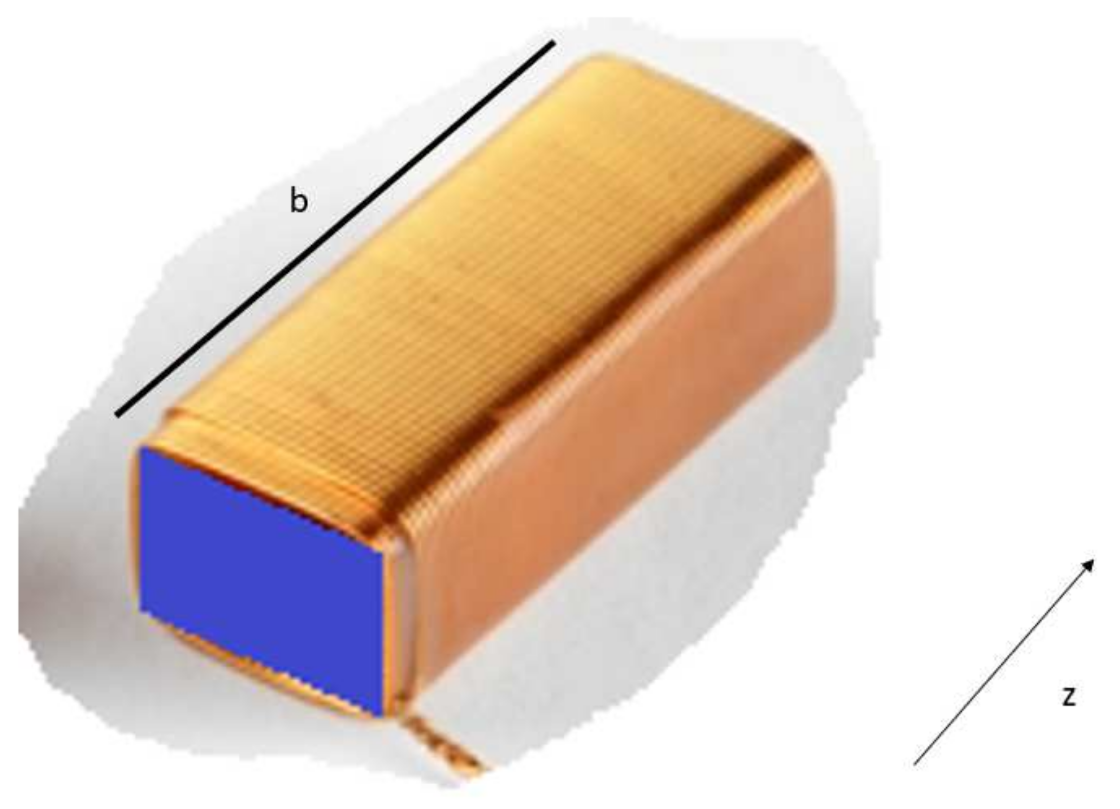
Considering an electret of thickness d and area of $a\times b$, the electret is put inside a tight superconductive winded coil (see Figure 2 and Figure 3).

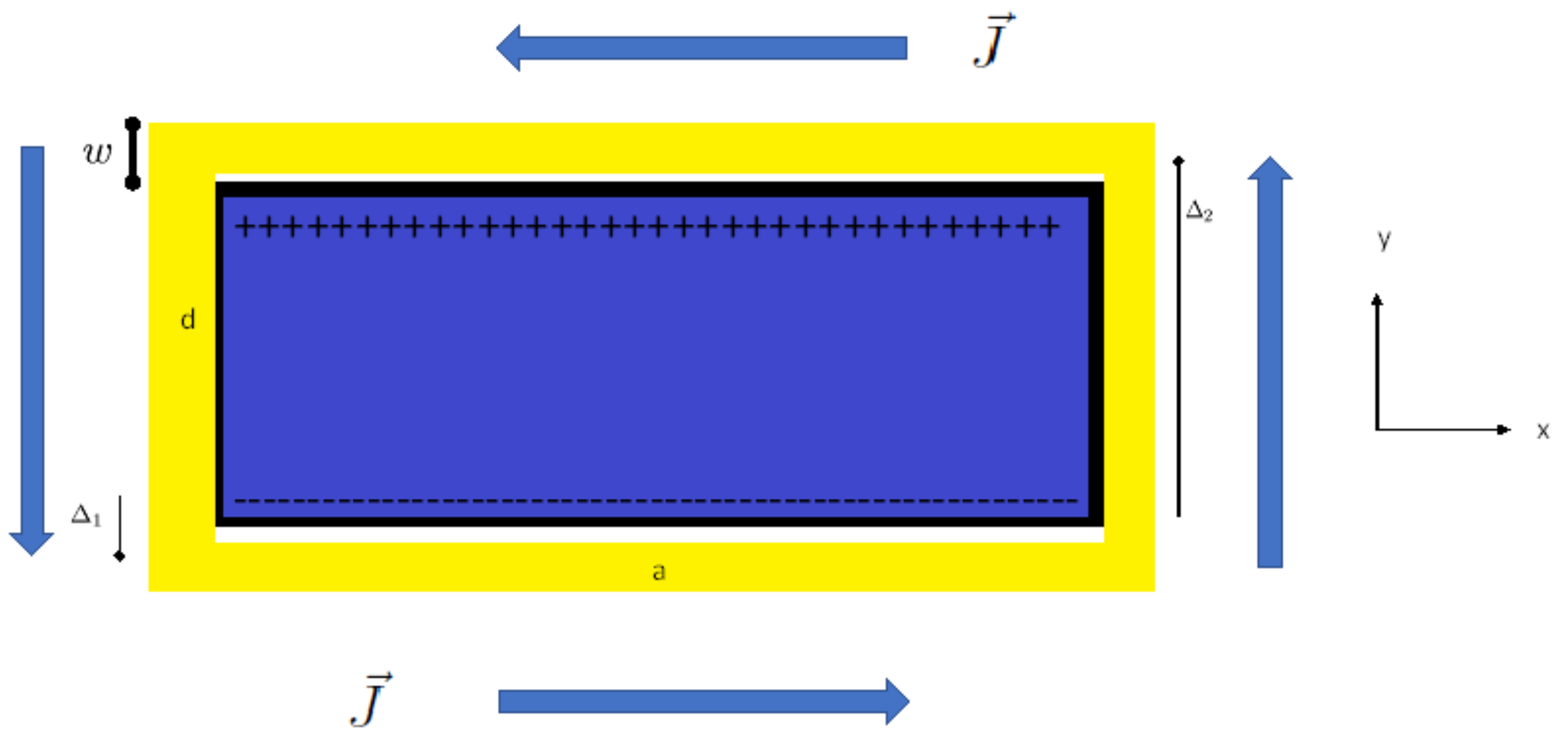
As the current in the x direction is close to the negative charge, it makes a considerable contribution to the momentum equation Equation (87), while the return current, which is far away from the negative charge, makes a relatively small contribution. The situation is reversed with regard to the positive charge; here, the return current makes the main contribution. Hence, the total momentum contribution is doubled with respect to the current flowing in the x direction and interacting with negative charge alone. The current flowing in the y direction does not contribute to the momentum, as the contribution from the current flowing upwards is exactly balanced by the contribution of the current flowing downwards. Let us look at the negative charge layer in Figure 3. We shall model this as a surface charged layer in the plane $y=0$ with a surface charge density $\sigma$ such that

$${\rho }_1(x_1,y_1,z_1)=-\sigma \delta \left(y_1\right)\left\{\begin{array}{cc}1& -\frac{a}{2}<x_1<\frac{a}{2},-\frac{b}{2}<z_1<\frac{b}{2}\\ 0& \mathrm{else}\end{array}\right.$$

(92)

in the above $\delta \left(y_1\right)$ is a Kronecker delta.

$${\overrightarrow{J}}_2(x_2,y_2,z_2)=\widehat{x}{J}_{0}w\delta (y_2+\mathsf{\Delta })\left\{\begin{array}{cc}1& -\frac{a}{2}<x_2<\frac{a}{2},-\frac{b}{2}<z_2<\frac{b}{2}\\ 0& \mathrm{else}\end{array}\right.$$

(93)

where $J_0$ is the current density, w is the width of the winding, $\widehat{x}$ is a unit vector in the x direction and $\mathsf{\Delta }$ is the distance of the current plane from the negative charge plane. Obviously, there is a difference between the $\mathsf{\Delta }$ of the current, ${\mathsf{\Delta }}_1$, and the return current, ${\mathsf{\Delta }}_2$. The integrated current flowing through the system is the following:

$$I=J_{0}wb.$$

(94)

However, the current flowing through each single wire depends on the winding number $N_w$:

$$I_c=\frac{I}{N_w}$$

(95)

Plugging Equation (92) and Equation (93) into Equation (87), we arrive at the following momentum equation:

$$\overrightarrow{P}=\frac{{\mu }_0}{4\pi }\sigma J_{0}w\widehat{x}{\int }_{-\frac{a}{2}}^{+\frac{a}{2}}d{x}_1{\int }_{-\frac{b}{2}}^{+\frac{b}{2}}d{z}_1{\int }_{-\frac{a}{2}}^{+\frac{a}{2}}d{x}_2{\int }_{-\frac{b}{2}}^{+\frac{b}{2}}d{z}_2\frac{1}{R}.$$

(96)

such that

$$R=\sqrt{{(x_1-x_2)}^2+{(z_1-z_2)}^2+{\mathsf{\Delta }}^2}.$$

(97)

Defining the dimensionless variables,

$$x_1^{\prime }=\frac{x_1}{a},z_1^{\prime }=\frac{z_1}{b},x_2^{\prime }=\frac{x_2}{a},z_2^{\prime }=\frac{z_2}{b},R^{\prime }=\frac{R}{\mathsf{\Delta }},a^{\prime }=\frac{a}{\mathsf{\Delta }},b^{\prime }=\frac{b}{\mathsf{\Delta }}.$$

(98)

we may write the following:

$$\overrightarrow{P}=\frac{{\mu }_0}{4\pi }\sigma J_{0}wa{b}^2\tilde{\mathsf{\Lambda }}(a^{\prime },b^{\prime })\widehat{x}.$$

(99)

The function $\tilde{\Lambda }(a^{\prime },b^{\prime })$ is dimensionless and depends on the dimensionless quantities $a^{\prime },b^{\prime }$. It can be evaluated using the quadruple integral:

$$\tilde{\mathsf{\Lambda }}(a^{\prime },b^{\prime })\equiv {\int }_{-\frac{1}{2}}^{+\frac{1}{2}}d{x}_1^{\prime }{\int }_{-\frac{1}{2}}^{+\frac{1}{2}}d{z}_1^{\prime }{\int }_{-\frac{1}{2}}^{+\frac{1}{2}}d{x}_2^{\prime }{\int }_{-\frac{1}{2}}^{+\frac{1}{2}}d{z}_2^{\prime }\frac{a^{\prime }}{R^{\prime }}.$$

(100)

in which

$$R^{\prime }=\sqrt{a^{\prime 2}{(x_1^{\prime }-x_2^{\prime })}^2+b^{\prime 2}{(z_1^{\prime }-z_2^{\prime })}^2+1}.$$

(101)

We shall attempt to perform at least part of this integration analytically. For this, we shall define the auxiliary function:

$$\begin{array}{ccc}\hfill \tilde{\mathsf{\Gamma }}(a^{\prime },b^{\prime },x_2^{\prime },z_2^{\prime })& \equiv & {\int }_{-\frac{1}{2}}^{+\frac{1}{2}}d{x}_1^{\prime }{\int }_{-\frac{1}{2}}^{+\frac{1}{2}}d{z}_1^{\prime }\frac{a^{\prime }}{R^{\prime }}\hfill \\ \hfill \Rightarrow \tilde{\Lambda }(a^{\prime },b^{\prime })& =& {\int }_{-\frac{1}{2}}^{+\frac{1}{2}}d{x}_2^{\prime }{\int }_{-\frac{1}{2}}^{+\frac{1}{2}}d{z}_2^{\prime }\tilde{\mathsf{\Gamma }}(a^{\prime },b^{\prime },x_2^{\prime },z_2^{\prime }).\hfill \end{array}$$

(102)

We shall now make a change of variables:

$$x=x_1^{\prime }-x_2^{\prime },z=z_1^{\prime }-z_2^{\prime },$$

(103)

such that

$$\begin{array}{ccc}\hfill \tilde{\mathsf{\Gamma }}(a^{\prime },b^{\prime },x_2^{\prime },z_2^{\prime })& =& {\int }_{-\frac{1}{2}-x_2^{\prime }}^{+\frac{1}{2}-x_2^{\prime }}dx{\int }_{-\frac{1}{2}-z_2^{\prime }}^{+\frac{1}{2}-z_2^{\prime }}dz\frac{a^{\prime }}{R^{\prime }}\hfill \\ \hfill R^{\prime }& =& \sqrt{a^{\prime 2}{x}^2+b^{\prime 2}{z}^2+1}.\hfill \end{array}$$

(104)

Finally, we define the following:

$$\begin{array}{ccc}\hfill \mathsf{\Psi }(a^{\prime },b^{\prime },x,z_2^{\prime })& \equiv & {\int }_{-\frac{1}{2}-z_2^{\prime }}^{+\frac{1}{2}-z_2^{\prime }}dz\frac{a^{\prime }}{R^{\prime }}\hfill \\ \hfill \Rightarrow \tilde{\mathsf{\Gamma }}(a^{\prime },b^{\prime },x_2^{\prime },z_2^{\prime })& =& {\int }_{-\frac{1}{2}-x_2^{\prime }}^{+\frac{1}{2}-x_2^{\prime }}dx\mathsf{\Psi }(a^{\prime },b^{\prime },x,z_2^{\prime }).\hfill \end{array}$$

(105)

The function $\mathsf{\Psi }$ can be integrated analytically by introducing the new variable:

$$z^{\prime \prime }=\frac{b}{a}\frac{z}{\sqrt{x^2+a^{\prime -2}}}$$

(106)

in terms of which

$$\begin{array}{ccc}\hfill \mathsf{\Psi }(a^{\prime },b^{\prime },x,z_2^{\prime })& =& \frac{a}{b}{\int }_{z_1^{\prime \prime }}^{z_2^{\prime \prime }}d{z}^{\prime \prime }\frac{1}{\sqrt{1+z^{\prime \prime 2}}}=\frac{a}{b}\left[\mathrm{arcsinh}\left(z_2^{\prime \prime }\right)-\mathrm{arcsinh}\left(z_1^{\prime \prime }\right)\right]\hfill \\ \hfill z_1^{\prime \prime }& =& \frac{b}{a}\left(\frac{-\frac{1}{2}-z_2^{\prime }}{\sqrt{x^2+a^{\prime -2}}}\right),z_2^{\prime \prime }=\frac{b}{a}\left(\frac{+\frac{1}{2}-z_2^{\prime }}{\sqrt{x^2+a^{\prime -2}}}\right).\hfill \end{array}$$

(107)

Unfortunately, the calculation of $\tilde{\mathsf{\Gamma }}$ and $\tilde{\mathsf{\Lambda }}$ can only be done numerically.

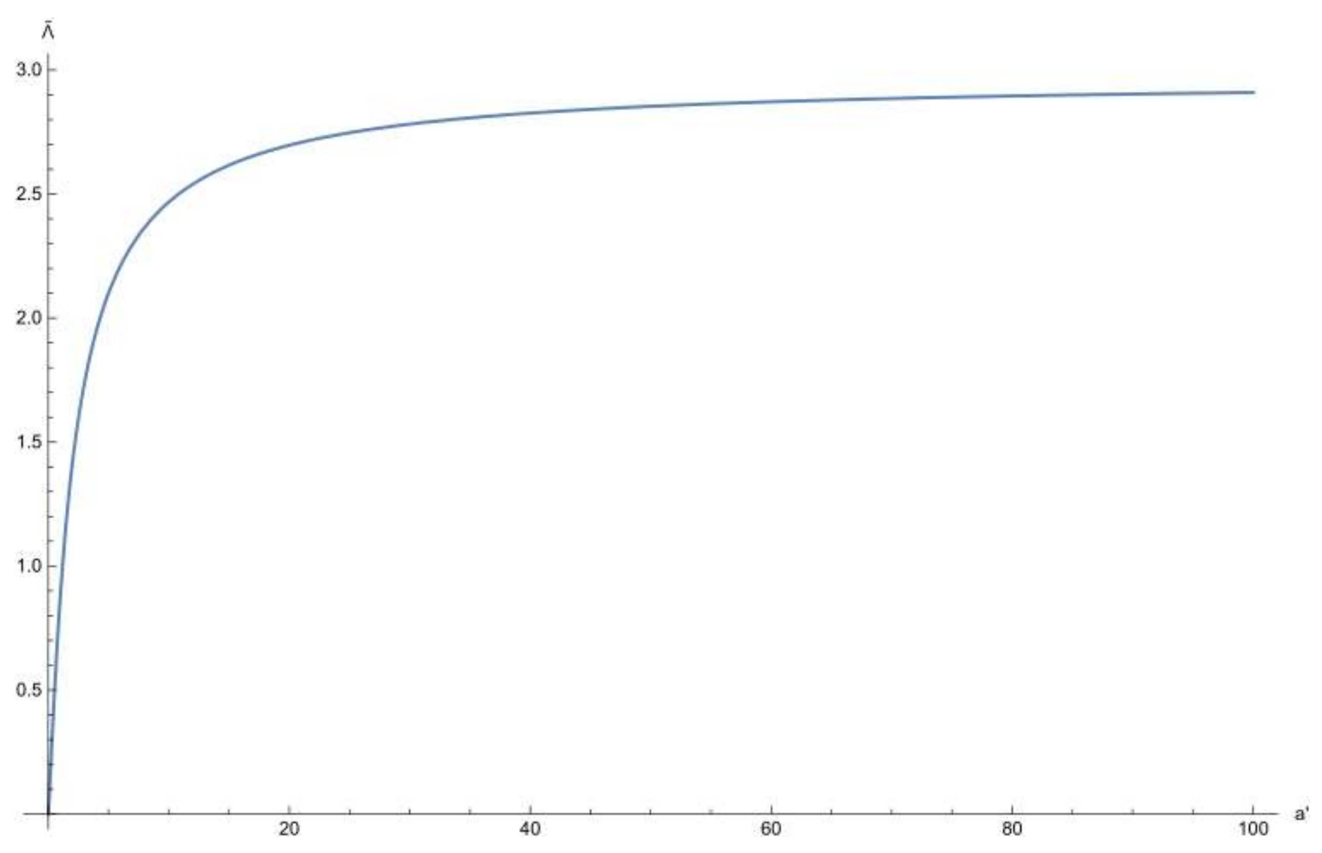
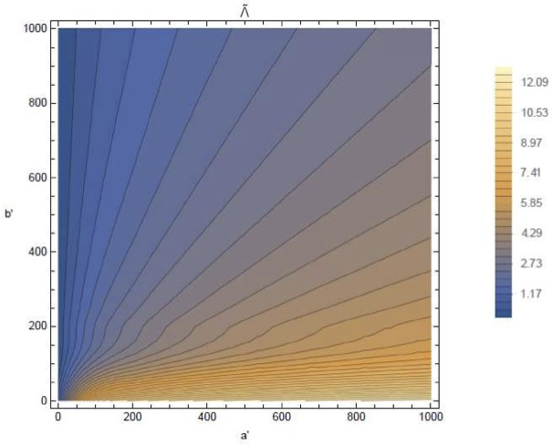
For the case $b^{\prime }=a^{\prime }$, the function $\tilde{\mathsf{\Lambda }}$ is a single variable function depicted in Figure 4.

It can be seen that for $a^{\prime }=0$, the function is null, while for $a^{\prime }=\infty$ it approaches $2.973\sim 3$. Hence, if the ratio of the size of the engine to the winding width is about 20 and $d\sim a$, one does not lose a significant amount of force and momentum due to the return current. However, looking at the case $b^{\prime }\ne a^{\prime }$ depicted in Figure 5, we see an obvious advantage for a slender relativistic motor in the direction of motion.

We also point out that the return current interacts symmetrically with the positive charge in a beneficial way, as both the sign of the charge and the direction of the current are reversed (see Figure 3). This doubles the momentum gain such that according to Equation (99), we have the following:

$${\overrightarrow{P}}_T=\frac{{\mu }_0}{2\pi }\sigma J_{0}wa{b}^2\left(\tilde{\Lambda }(\frac{a}{{\mathsf{\Delta }}_1},\frac{b}{{\mathsf{\Delta }}_1})-\tilde{\Lambda }(\frac{a}{{\mathsf{\Delta }}_2},\frac{b}{{\mathsf{\Delta }}_2})\right)\widehat{x}.$$

(108)

The quantities ${\mathsf{\Delta }}_1$ and ${\mathsf{\Delta }}_2$ are defined through Figure 3 and we thus expect the following:

$${\mathsf{\Delta }}_1=\frac{w}{2},{\mathsf{\Delta }}_2=\frac{w}{2}+d.$$

(109)

The force produced by the relativistic engine depends on the rise time of the current which can be increased gently or abruptly:

$${\overrightarrow{F}}_T=\frac{d{\overrightarrow{P}}_T}{dt}=\frac{{\mu }_0}{2\pi }\sigma \frac{d{J}_0}{dt}wa{b}^2\left(\tilde{\Lambda }(\frac{a}{{\mathsf{\Delta }}_1},\frac{b}{{\mathsf{\Delta }}_1})-\tilde{\Lambda }(\frac{a}{{\mathsf{\Delta }}_2},\frac{b}{{\mathsf{\Delta }}_2})\right)\widehat{x}.$$

(110)

We choose three different configurations of a relativistic motor: one is a size of standard car and its parameters are described in the first column of

Table 1. Maximal momentum gained by a relativistic motor for three cases of parameters. We assume an extreme case of charge density $\sigma$ = 3.7 × 10${}^{-3}$ Coulomb/${\mathrm{m}}^2$ (see Section 3.4), and current density $J_0$ = 5 × 10${}^7$ Ampere/${\mathrm{m}}^2$ (see Section 3.5).

	Car	Rocket Size Engine	Giant Cube	Units
a	6	200	1000	m
b	2	10	1000	m
d	1	10	1000	m
w	0.2	0.4	0.4	m
$P_T$	0.3	868	3.1 × ${10}^7$	kg m/s

, the second describes a considerably larger motor which may be suitable for space travel is given in the second column of Table 1, and the third column describes a cube of immense dimensions.

We see that, despite the extreme parameters, the maximum momenta gained are quite modest. This is a direct result of the phenomena of dielectric breakdown. Nevertheless, for the purpose of demonstration, the car configuration of Table 1 can be built and measured in a laboratory to experimentally verify its performance.

5. The Nano Relativistic Motor

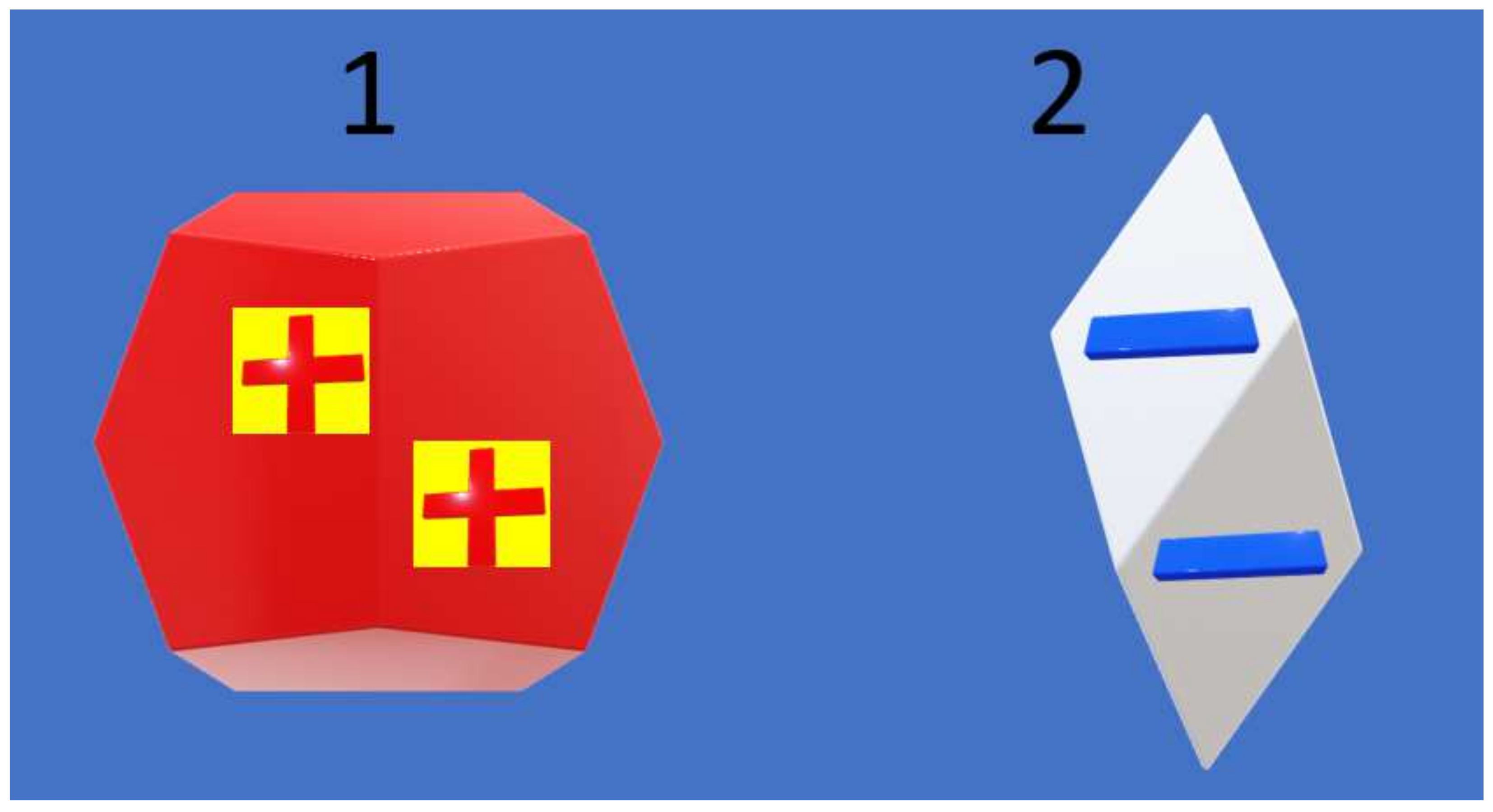
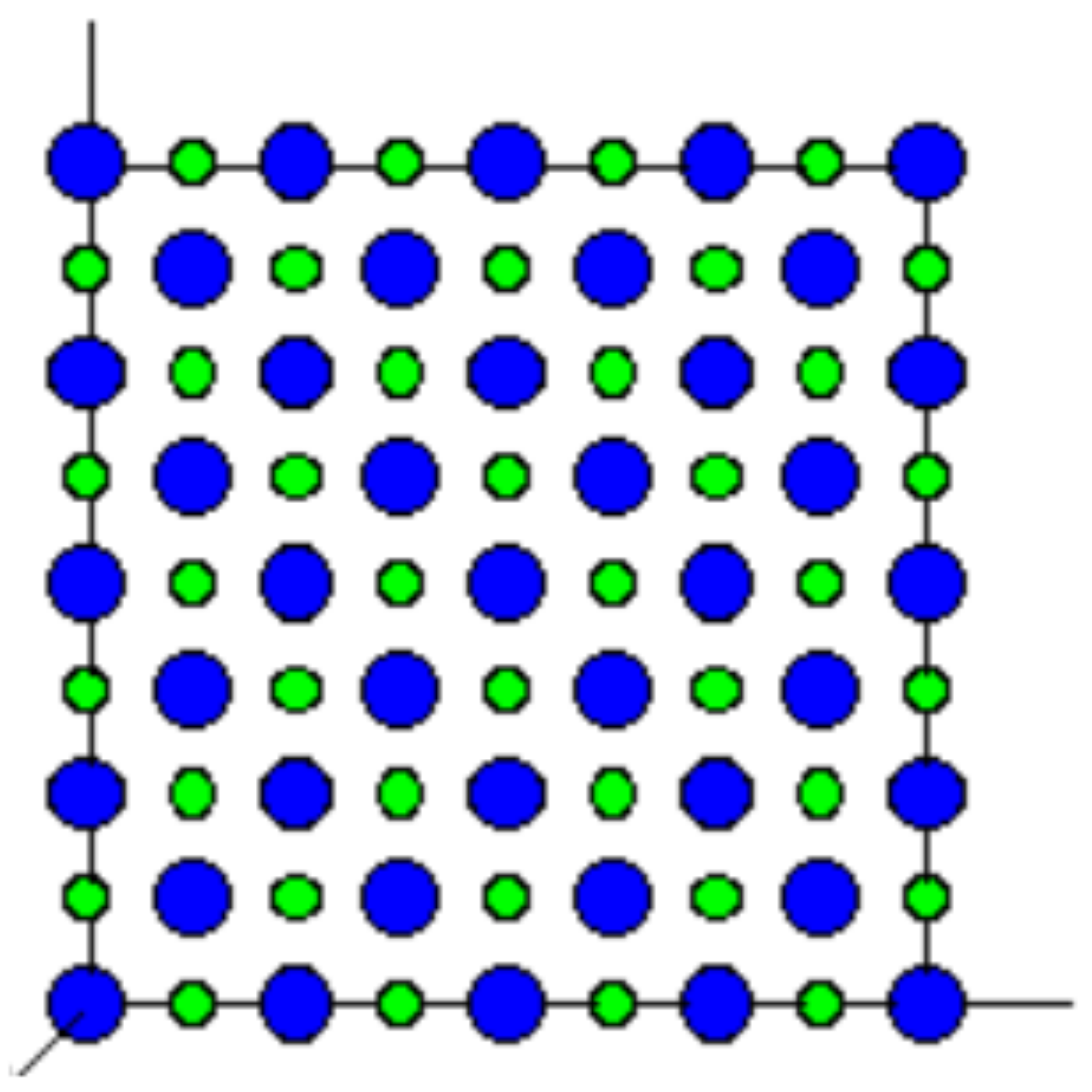
In the previous section, we showed that intrinsic parameter limitations, especially dielectric breakdown, lead to a somewhat modest amount of momenta that can be gained by a relativistic motor. However, it seams that in the microscopic domain, this limitation is rather relaxed. For example, consider ionic crystals such as the prevalent table salt: $N{a}^{+}C{l}^{-}$. This salt solidifies to a face-centered cubic lattice in which the lattice constant is $l=564.02$ pm. Taking, for example, the 100 plane of this lattice (see Figure 6), we can see that the charge density is periodical in which in each half unit cell, we have a surface charge density of $\pm 2\mathrm{Coulomb}/{\mathrm{m}}^2$. This is, of course, a thousand times larger than the available macroscopic charge densities (see Section 3.4); however, on the macroscopic average, this leads to a null charge density.

To see how we can circumvent this unfortunate reality, we investigate Equation (87), calculating the spatial Fourier transform of the scalar potential and the current density such that

$$\begin{array}{ccc}\hfill {\mathsf{\Phi }}_1\left(\overrightarrow{k}\right)& =& {\int }_{-\infty }^{+\infty }{\int }_{-\infty }^{+\infty }{\int }_{-\infty }^{+\infty }{\mathsf{\Phi }}_1\left(\overrightarrow{x}\right)e^{-i\overrightarrow{k}·\overrightarrow{x}}{d}^{3}x\hfill \\ \hfill {\overrightarrow{J}}_2\left(\overrightarrow{k}\right)& =& {\int }_{-\infty }^{+\infty }{\int }_{-\infty }^{+\infty }{\int }_{-\infty }^{+\infty }{\overrightarrow{J}}_2\left(\overrightarrow{x}\right)e^{-i\overrightarrow{k}·\overrightarrow{x}}{d}^{3}x.\hfill \end{array}$$

(111)

Using the theorem of Parseval [25], we may now write Equation (87) in the following form:

$$\overrightarrow{P}\left(t\right)=-\frac{1}{c^2{\left(2\pi \right)}^3}{\int }_{-\infty }^{+\infty }{\int }_{-\infty }^{+\infty }{\int }_{-\infty }^{+\infty }{d}^{3}k{\mathsf{\Phi }}_1^{*}\left(\overrightarrow{k}\right){\overrightarrow{J}}_2\left(\overrightarrow{k}\right)$$

(112)

In this form, it is obvious that a microscopic distribution of periodic charge density is beneficial if it is accompanied by a current density distribution of the same period. How can we obtain such a microscopic charge density distribution? To this end, we remind the reader that microscopic currents are associated with the electronic motion and electronic spin. The magnetization $\overrightarrow{M}$ is related to the magnetization current ${\overrightarrow{J}}_M$ by the following formula [14,15]:

$${\overrightarrow{J}}_M\equiv \overrightarrow{\nabla }\times \overrightarrow{M}.$$

(113)

We may replace in Equation (86), Equation (87) and Equation (112) $\overrightarrow{J}$ by ${\overrightarrow{J}}_M$ to obtain a similar effect. Furthermore, the magnetization $\overrightarrow{M}$ is related to the microscopic dipole moments ${\overrightarrow{m}}_i$ through the following:

$$\overrightarrow{M}\equiv \frac{1}{V}\sum _i{\overrightarrow{m}}_i.$$

(114)

in which we sum over all dipoles and divide by the sample volume V. In known magnetic materials, for example, iron, magnetic dipole moments are a consequence of the atom spin configuration. For example, in the case of $\alpha$-iron, the spins of two unpaired electrons in each atom generally align with the spins of its closest neighbors. The reason for this is that the orbitals of those two electrons ($d_{z^2}$ and $d_{x^2-y^2}$) do not point in the direction of neighboring atoms in the lattice and since this is the case, are not involved in metallic bonding. We thus hypothesize that the ideal structure of a relativistic motor involves an ionic lattice in which one species of atom (for example, the positively charged) involve free spins that can be manipulated by an external magnetic field, thus creating a relativistic engine effect which can be easily manipulated in three axes. The details of such an engine are beyond the scope of the current paper.

6. Discussion

In this paper, we have shown that, in general, Newton’s third law is not compatible with the principles of special relativity, and the total force on a two-charged body system is not zero. Still, momentum is conserved if one takes the field momentum into account, and the same is true for energy.

The main results of this paper are given by Equation (82) and Equation (83), which describe the total relativistic force for charged bodies. Not all configurations of charged relativistic motors were analyzed here due to space limitations. We have concentrated our efforts on a system in which one part is charged and the second part carries current. It is noticed that the charge relativistic motor is many orders of magnitude more powerful than an uncharged relativistic motor. Still, it is shown that the limitations of dielectric breakdown and current density lead to a rather modest momentum generated by the engine at the macroscopic level.

Those limitations can be somewhat relaxed at the atomic level, as the surface charge density for typical ionic crystals is three orders of magnitude larger than what can be achieved at the macroscopic level. Thus, future work will concentrate on the development of nano relativistic engines. Other open subjects are exploring additional possible charged relativistic configurations, as suggested by Equation (83), and studying in detail momentum and energy transformation from the electromagnetic to the mechanical elements of the motor.

Obviously, conducting experimental verification of the suggested relativistic engine is highly desirable in order to corroborate the ideas presented in the current paper. This is also left as a task for the future.

7. Conclusions

To conclude, we make a comparison between the relativistic motor and other types of electromagnetic engines. A photon engine emits photons backwards and thus propels itself forward. It may be a powerful laser or a radio-frequency cavity [26] (the only difference between those two cases are the energy and momentum of a single photon). To reach a momentum p, using a photon engine, one needs an energy of $E_p=pc$, while for a relativistic engine, an energy of $E\sim \frac{1}{2}pv$ suffices. The ratio is $\frac{E_p}{E}=\frac{2c}{v}$, which is a huge number for non-relativistic speeds.

Of course, standard electric cars today (Tesla, for example) can reach significant speed and momentum, but unlike the relativistic motor, they need a road to push against; otherwise, no motion is possible.