A Kinematical Analysis of the Flap and Wing Mechanism of a Light Sport Aircraft Using Topological Models

Abstract

In this, paper, we propose a method of kinematic analysis of a planar mechanism with application to the flap and wing mechanism of a light sport aircraft. A topological model is used to describe a mechanical system, which is a model that allows the study of the maneuverability of the system. The proposed algorithm is applied to determine the velocity and acceleration field of this multibody mechanical system. The graph associated with the mechanical system is generated in a new formulation and based on it, the fundamental loops of the graph are identified (corresponding to the independent loops of the mechanism), the equations for closing vectorial contours are written, and the kinematic conditions for determining velocities and accelerations and the associated linear systems are solved, which provides the field of speeds and accelerations. Graph Theory is applied at a kinematic level and not at a dynamic level, as in previous studies. A practical application for the kinematic analysis of the control mechanism of a light aircraft illustrates the proposed method.

1. Introduction

Graph theory, strongly developed in the middle of the last century, has proven its usefulness in many fields of engineering [1]. One of the areas in which this theory has been very successful is the theory of electrical circuits. Graph theory is used for studying electrical circuits (in fact for systematization of description and automation of calculations), by associating a graph with each real circuit, and then by using the theorems of this theory, algorithms and numerical procedures can be formulated. Studies have demonstrated the advantages of using graphs to describe electrical circuits [2,3]. The success of the method has also inspired mechanical engineers, who have applied the method, in different forms, for kinematic and dynamic analyses of mechanisms. In this paper, we show that graph theory can be used successfully to describe a planar mechanism with joints and that the application of the results can be extremely useful in kinematic analysis. The problem that arises is the suitable association of the notions, descriptions, and theoretical results obtained in graph theory with the notions and description of planar mechanisms. If this is done properly, then, performing the kinematic analysis can be significantly facilitated by using some previously known results. This approach has significant advantages for designers and contributes to the development of a useful description for engineers. In this way, kinematic liaisons between elements and fundamental equations of mechanics can be written using the formalism of graph theory and some properties of written relations can be determined by virtue of the known results from graph theory.

The synthesis of mechanisms is a basic stage in the design of a new device, which, in general, is conducted using traditional methods that involve time consuming operations for a designer. Graph theory allows the algorithmization of the synthesis process in certain cases, as presented in [4]. A graph was associated with the mechanism that took into account the kinematic chains considered. A tree was identified in this graph and graph theory was used for the synthesis of the studied mechanism. Examples were also presented that proved the effectiveness of the method. An extended matrix was generated using the formalism of graph theory in [5,6], which contained the complete characterization of a planar mechanism, with all the necessary information for an analysis related to topology and geometry. This proposed representation allowed one to optimize the design of the mechanism, as all the information regarding the mechanism was stored together and was easily accessible, enabling a topological and dimensional synthesis of the mechanism. Thus, optimization algorithms could be formulated using, for example, metaheuristic algorithms. An example was also presented for the design of a trajectory tracking mechanism. Therefore, the results proved that the matrix method, based on graph theory, represented a useful, organized, and flexible tool for the design of a mechanical system used in engineering.

A symbolic formulation based on Lie groups and graph theory for the dynamic analysis of robotic structures was presented in [7]. The results were equivalent to the traditional Newton–Euler equations of motion but the computational effort was decreased substantially. This type of analysis can be applied to any robotic structure that does not have closed kinematic chains. An open kinematic chain manipulator or robotic hands (currently, very trendy) or humanoid robots can be included in this method of analysis. The results can still be used to control such systems. The necessary information is entered into a matrix that facilitates easy mathematical manipulations for obtaining simulation, analysis, or identification algorithms. An application on a robot with seven degrees of freedom, and then on a robot with sixteen degrees of freedom illustrated the method. A comparison with the MSC/ADAMS simulation package demonstrated the advantages of the method. Of course, the results can be extended, carefully, to closed kinematic loops, encountered in planar mechanisms, and therefore, consequently, any type of mechanism with tree structure can be analyzed [8].

A study on the use of graph theory investigated the power flow of an engine that drives transmission systems used in tracked vehicles [9]. By studying the transmission of power flows to two parts of the vehicle, an efficient and more useful solution was obtained than by traditional methods, especially in the case of complex mechanical transmission systems with multiple input and multiple outputs.

An exhaustive method for designing new mechanisms for reflector antennas, based on graph theory was presented in [10]. The mechanism consisted of elements connected by joints. Graph theory was used to present the connections between elements and based on this representation, it was possible to automate the calculations and identify the optimal solution for this problem.

An interesting presentation of the possible applications of graph theory in the study of plane mechanisms was presented in [11]. Topological graphs were introduced, such as a simple graph, a bicolor graph, and a tricolor graph. These graphs described the topological relationships that existed between the different kinematic pairs and defined the connections that existed between these elements. The incident matrix and the fundamental loop matrix represented the mathematical description of the structure and connections of a plane mechanism, therefore, it was easier to model the mechanism to solve the kinematical analysis. According to these models, a structural and kinematic study of the mechanism was performed and some examples illustrated the proposed method.

For the optimal synthesis of vehicle suspension mechanisms using an expert system, graph theory has been proven to be very useful [12]. A database with several types of suspension mechanisms was used and an algorithm for choosing the optimal solution from the database was developed. The goal was to choose a suitable suspension from several new suspension configurations in order to ensure ease of maintenance and vibration damping efficiency.

A method that proved to be very useful for dynamic analyses of robotic mechanisms was developed using graph theory in [13]. A hierarchy was made of the connections that existed between the different elements of a robotic mechanism. The procedure was illustrated in the analysis of a manipulator with two degrees of freedom.

Topological methods mentioned in the design of a car windshield wiper mechanism were used in [14]. After specifying the objectives pursued as well as the constraints to be observed, kinematic structures useful to the designer were generated. Thus, several mechanisms were selected that could meet the requirements of the project. Constraints and objective functions were used for optimization in order to determine the best solution from an engineering point of view.

A description that fits very well with the topological description of a planar mechanism is Assur graphs, a method that uses a table to enter information about the structure of the mechanism (the canonical form of planar linkages). This description is suitable for all planar mechanisms. Starting from the Assur groups, well known in traditional kinematics, [15] proposed a mathematical method, with demonstrations of useful theorems, for the description and analysis of a planar mechanism. It has been found that most studies that use graph theory in the analysis of mechanisms deal with planar mechanisms.

Currently, the designs of mechanical structures used in engineering practice use sophisticated methods of optimization and topological analysis to establish the optimal version of a project. A new method for approaching such problems was presented in [16]. A genetic algorithm was used to solve the problem of topological synthesis and the methods shown were illustrated by examples.

In engineering practice, there is no unitary approach for modeling a complex mechanism consisting of several kinematic chains. In these cases, a consistent and systematic approach is useful, using the information provided by the topology of the studied system. An attempt to systematize and unify the kinematic formulations was made in [17]. Geometric constraints and kinematic constraints were applied to independent loops.

The analysis of an exoskeleton using topological descriptions and the theory of forks was conducted in [18]. The contour equation method was used to analyze the mechanical system and Lagrange equations were used to write the equations of motion. The model used for the calculation was verified by using Adams commercial software.

The contributions of the above-mentioned studies show that researchers have long been concerned with the study of planar mechanisms with the use of graph theory and topological analysis. These methods are convenient for describing the structure of a mechanism. Several methods of analysis have been developed using these notions. In this paper, we use known theorems and results from graph theory, but the method of constructing graphs is different from those presented in most studies. A loop of the graph associated with the mechanism consists of a closed vector contour. The graph is the perfect representation of the mechanism, in which the vertices represent the cylindrical joints, and the edges represent the bars. In this way, using this description and the traditional theorems from graph theory, a kinematic analysis of the mechanism is made easier and the results can be conveniently systematized. The presented theory has advantages in the case of mechanisms that are made up of several kinematic chains.

The solution presented in this paper is the subject of a patent registered by the authors of the paper [19]. An analysis method, developed and applied prior to the writing of this paper, allowed us to choose, from a larger set of possible mechanisms for transmitting motion, a mechanism that would meet several engineering requirements. For this, we used the specialized literature presented in the Introduction and also two decades of practical experience by one of the authors. Thus, any mechanism, no matter how complicated, can be described, structurally, through an incidence matrix, and the calculations can be performed based on an algorithm that describes the operations performed. In this way, the kinematic analysis time of a mechanism can be significantly shortened, which is an important advantage in the design stage of a mechanism.

The advantages of the proposed mechanism are:

• The mechanism achieves steering angles up to 70°, from negative down to the wing string, and is superior to traditional solutions that achieve steering angles up to 40°;
• The components of the mechanism have constructive and technological simplicity;
• The steering angles are not achieved by rotations around a hinge (fixed axis of rotation) located in the wing structure, however, they are achieved by complex movements using kinematic elements for constructing the mechanism of control flaps;
• The construction of the aircraft fuselage allows access to installations for overhauls and repairs, enabling required maintenance and upkeep without a high cost;
• The light aircraft has a simple and fast response structure, is safe and reliable, and has good flight control, lifting performance, as well as stability of movement;
• This flywheel control mechanism can be used for short-distance take-offs and landings over a short time;
• The mechanism has a robust construction and unpretentious manufacturing technology, which implies low execution costs.

In this paper, we analyze a proposed mechanism for controlling flaps and ailerons of a light aircraft designed for sport activities, which must have excellent maneuverability and stability. For the kinematic analysis of the mechanism, an analysis method is applied using a topological model for the description of the system and the results are obtained using graph theory, which have both been successfully applied in electrical circuit theory. On the basis of the topological description, an algorithm for determining the field of velocities and accelerations of the elements of the mechanism is obtained, which can be used for a systematic study with reduced effort. For a complex mechanism, such as the one presented in this paper, this can lead to significant time savings. The experience gained in the study of electrical circuits, using graph theory, as previously presented, proves this. Next, we present a description of the proposed method.

The main advantage of the method is the possibility of algorithmizing the process and, as a result, the possibility of unitary treatment of such problems. The topology describes the structure of the mechanical system, and then it is possible to use calculation programs that automate the results, without using, for each mechanism, elementary geometric and trigonometric methods for solving them.

The dynamics of the system and the aerodynamic forces that appear have not been analyzed in this paper, the problem being partially treated in [20].

The proposed method can help the design process by reducing the computation time required. In this way, several calculation options can be checked in a short time period and the best option can be selected, considering different constructive criteria.

The structure of this paper is as follows: First, we present the topological model useful for the qualitative and quantitative analysis of the mechanism. Then, we present an application of the method to a command mechanism of the flaps on a light sport aircraft.

2. Graph Associated with a Planar Mechanism with Joints

2.1. Elementary Notion Used in Graph Theory

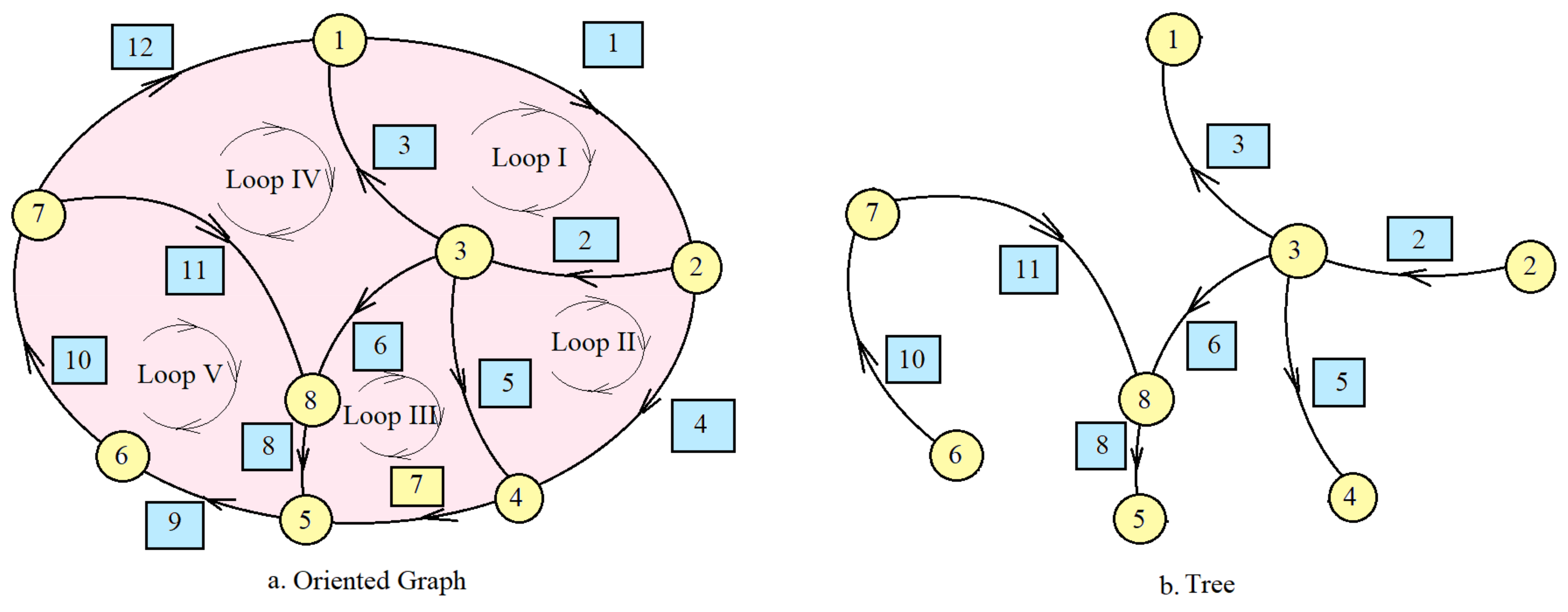
A graph is made up of vertices and edges (links or lines) (Figure 1a). The traditional representation of a graph is a diagram with circles for the vertices joined by lines for the edges. If the sides are associated with a sense of traversal, then, it is referred to as an oriented graph. A vertex is the connection point of at least two edges. An edge represents the connection between two vertices. A graph is called connected if it can pass from any node of the circuit, going through exclusive edges of the graph, to any other node of it. A graph that is unconnected can be transformed into a connected one by adding edges.

The loop represents the totality of the edges that form a closed circuit. In Figure 1a, five loops of the graph are presented but there are more than five circuits in this graph; only the main and obvious circuits of the graph are presented.

The tree represents the connection between all the vertices of a circuit (graph) without forming loops. In Figure 1b, a tree of the graph is shown. It is worthwhile to mention that the tree of a graph can be obtained in several ways, and therefore the tree is not unique.

Mathematically, a graph is a structure G = (V, E) consisting of a set of vertices V and a set of edges E. G is finite if V and E are finite sets. In this paper, we will naturally consider only finite graphs.

The order of a graph is |V| = n, the number of vertices.

The size of a graph is |E| = l, the number of edges.

Let x, y ∈ V be two vertices. We say that x is the neighbor of y if E contains an edge from x to y. If G is oriented, y is the destination of an arc with source x.

The edges belonging to the tree are called branches. Noting with n the number of vertices of a graph and with l the number of edges, the branches satisfy the relation r_a = n − l.

It is called the independent loop, i.e., the loop that contains at least one edge that does not belong to the other loops.

The graphs serve to illustrate the topological properties of the mechanical systems and the matrices that are introduced serve to describe the quantitative properties of these properties.

In graph theory, for a quantitative description of topological properties, the procedure is as follows:

• Draw the oriented graph.
• Choose the main tree, build the independent loops on its base, and choose a direction for traversing each loop.
• Define the topological properties of the mechanical system by constructing the incidence matrix (defined below).

2.2. The Associated Graph and the Incidence Matrix

Let r + 1 be the number of vertices and s the number of edges of the obtained graph. The complete incidence matrix $\left[A\right]=\left[{\epsilon }_{ij}\right]$ for the given graph is the matrix of dimensions (r + 1) × s (s > r) with:

• ${\epsilon }_{ij}=1$ if side j is the incident at node i and comes out of the node;
• ${\epsilon }_{ij}=-1$ if side j is the incident at node i and enters the node;
• ${\epsilon }_{ij}=0$ if side j is not the incident at node i.

Therefore, $\left[A\right]$ looks like:

$$\begin{array}{l}\hspace{1em}\hspace{1em}nodes\backslash edges\\ \hspace{1em}\hspace{1em}\hspace{1em}\hspace{1em}\begin{array}{ccccc}1& \hspace{1em}2& \hspace{1em}3& \hspace{1em}\dots & s\end{array}\\ \left[A\right]=\begin{array}{c}1\\ 2\\ ⋮\\ \\ r+1\end{array}\left[\begin{array}{ccccc}{\epsilon }_{11}& {\epsilon }_{12}& {\epsilon }_{13}& \dots & {\epsilon }_{1s}\\ {\epsilon }_{21}& {\epsilon }_{22}& {\epsilon }_{23}& \dots & {\epsilon }_{2s}\\ ⋮& & & & ⋮\\ ⋮& & & & ⋮\\ {\epsilon }_{r+1,1}& {\epsilon }_{r+1,2}& {\epsilon }_{r+1,3}& \dots & {\epsilon }_{r+1,s}\end{array}\right]\end{array}$$

(1)

where:

$${\epsilon }_{ij}\in \left\{-1\hspace{0.17em}\hspace{0.17em},\hspace{0.17em}\hspace{0.17em}0\hspace{0.17em}\hspace{0.17em},\hspace{0.17em}\hspace{0.17em}1\hspace{0.17em}\hspace{0.17em}\right\}\hspace{1em};\hspace{1em}i=1,\hspace{0.17em}2,\hspace{0.17em}\dots ,\hspace{0.17em}r+1\hspace{1em};\hspace{1em}j=1,\hspace{0.33em}2,\hspace{0.17em}\dots ,\hspace{0.17em}s$$

(2)

For the graph presented in Figure 1a, the incidence matrix is:

$$\begin{array}{cc}\hfill & nodes\setminus branches\hfill \\ \hfill & \begin{array}{ccccc}1& 2& 3& 456789101112& \end{array}\hfill \\ \hfill & \left[A\right]=\begin{array}{c}1\\ 2\\ 3\\ 4\\ 5\\ 6\\ 7\\ 8\end{array}\left[\begin{array}{cccccccccccc}1& 0& -1& 0& 0& 0& 0& 0& 0& 0& 0& -1\\ -1& 1& 0& 1& 0& 0& 0& 0& 0& 0& 0& 0\\ 0& -1& 1& 0& 1& 1& 0& 0& 0& 0& 0& 0\\ 0& 0& 0& -1& -1& 0& 1& 0& 0& 0& 0& 0\\ 0& 0& 0& 0& 0& 0& -1& -1& 1& 0& 0& 0\\ 0& 0& 0& 0& 0& 0& 0& 0& -1& 1& 0& 0\\ 0& 0& 0& 0& 0& 0& 0& 0& 0& -1& 1& 1\\ 0& 0& 0& 0& 0& -1& 0& 1& 0& 0& -1& 0\end{array}\right].\hfill \end{array}$$

(3)

The matrix ${\left[A\right]}_a$ of rank r obtained by suppressing a row in $\left[A\right]$ is called the reduced incidence matrix. For the graph, presented in this section, it is:

$$\begin{array}{cc}\hfill & nodes\setminus branches\hfill \\ \hfill & \begin{array}{ccccc}1& 2& 3& 456789101112& \end{array}\hfill \\ \hfill & {\left[A\right]}_a=\begin{array}{c}1\\ 2\\ 3\\ 4\\ 5\\ 6\\ 7\end{array}\left[\begin{array}{cccccccccccc}1& 0& -1& 0& 0& 0& 0& 0& 0& 0& 0& -1\\ -1& 1& 0& 1& 0& 0& 0& 0& 0& 0& 0& 0\\ 0& -1& 1& 0& 1& 1& 0& 0& 0& 0& 0& 0\\ 0& 0& 0& -1& -1& 0& 1& 0& 0& 0& 0& 0\\ 0& 0& 0& 0& 0& 0& -1& -1& 1& 0& 0& 0\\ 0& 0& 0& 0& 0& 0& 0& 0& 0& -1& 1& 1\\ 0& 0& 0& 0& 0& -1& 0& 1& 0& 0& -1& 0\end{array}\right].\hfill \end{array}$$

(4)

We can choose a tree of this graph (Figure 1b). Selecting a tree in the presented graph allows a reordering and partitioning of ${\left[A\right]}_a$:

$${\left[A\right]}_a=[\left[A_t\right]\hspace{0.17em}⋮\hspace{0.17em}\left[A_l\right]\hspace{0.17em}]$$

(5)

so that the columns of $\left[A_t\right]$ correspond to the branches of the tree and the columns of $\left[A_l\right]$ correspond to the junctions (to the other edges, that attached to the chosen tree give the initial graph).

The complete matrix of the loops is the matrix $B_a=[b_{ij}]$ with:

• $b_{ij}=1$ if the branch j is part of loop i and its orientation coincides with the direction chosen for browsing the loop;
• $b_{ij}=-1$ if side j is part of loop i and its orientation is contrary to the direction chosen for browsing the loop;
• $b_{ij}=0$ if branch j is not part of loop i.

$$\begin{array}{l}\hspace{1em}\hspace{1em}loops\backslash branches\\ \hspace{1em}\hspace{1em}\hspace{1em}\hspace{1em}\begin{array}{ccccc}1& \hspace{1em}\hspace{1em}2& \hspace{1em}\hspace{1em}3& \hspace{1em}\dots & \hspace{1em}s\end{array}\\ {\left[B\right]}_a=\begin{array}{c}1\\ 2\\ ⋮\\ \\ n_b\end{array}\left[\begin{array}{ccccc}{\eta }_{11}& {\eta }_{12}& {\eta }_{13}& \dots & {\eta }_{1s}\\ {\eta }_{21}& {\eta }_{22}& {\eta }_{23}& \dots & {\eta }_{2s}\\ ⋮& & & & ⋮\\ ⋮& & & & ⋮\\ {\eta }_{nb+1,1}& {\eta }_{nb+1,2}& {\eta }_{nb+1,3}& \dots & {\eta }_{nb+1,s}\end{array}\right]\end{array}$$

(6)

where $n_b$ represents the total number of graph loops, ${\eta }_{ij}\in \left\{-1\hspace{0.17em}\hspace{0.17em},\hspace{0.17em}\hspace{0.17em}0\hspace{0.17em}\hspace{0.17em},\hspace{0.17em}\hspace{0.17em}1\hspace{0.17em}\hspace{0.17em}\right\}\hspace{1em};$ $i=1,2,\dots ,n_b\hspace{1em};$ $j=1,2,\dots .,s$. The rank of the matrix ${\left[B\right]}_a$ is s-r. The matrix ${\left[B\right]}_f$ having the rank s-r obtained from $\left[B\right]$ the retention of s-r linear independent lines is the matrix of the fundamental loops. Between ${\left[B\right]}_f$ and A there is the relation:

$${\left[B\right]}_f=[{[-{\left[A\right]}_t^{-1}{\left[A\right]}_l]}^T⋮\left[E\right]]$$

(7)

where $\left[E\right]$ represents the unit matrix having the dimension s-r.

For the graph presented in Figure 1a, the matrix of the fundamental loops is:

$$\begin{array}{l}\hspace{1em}\hspace{1em}loops\backslash edges\\ \begin{array}{cccccccccccc}1& 2& 3& 4& 5& 6& 7& 8& 9& 10& 11& 12\end{array}\\ {\left[B\right]}_a=\begin{array}{c}1\\ 2\\ 3\\ 4\\ 5\end{array}\left[\begin{array}{cccccccccccc}1& 1& 1& 0& 0& 0& 0& 0& 0& 0& 0& 0\\ 0& -1& 0& 1& -1& 0& 0& 0& 0& 0& 0& 0\\ 0& 0& 0& 0& 1& -1& 1& -1& 0& 0& 0& 0\\ 0& 0& -1& 0& 0& 1& 0& 0& 0& 0& -1& 1\\ 0& 0& 0& 0& 0& 0& 0& 1& 1& 1& 1& 0\end{array}\right]\end{array}$$

(8)

2.3. The Kinematic Equivalent of the Given Mechanism

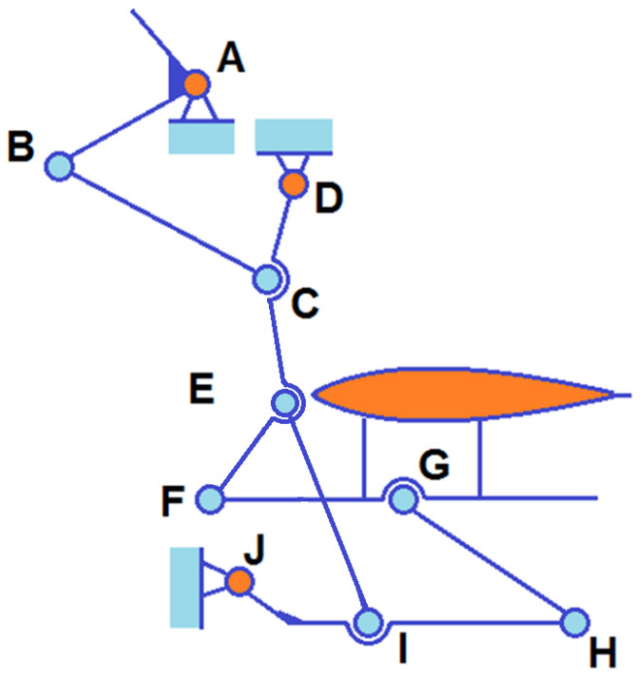
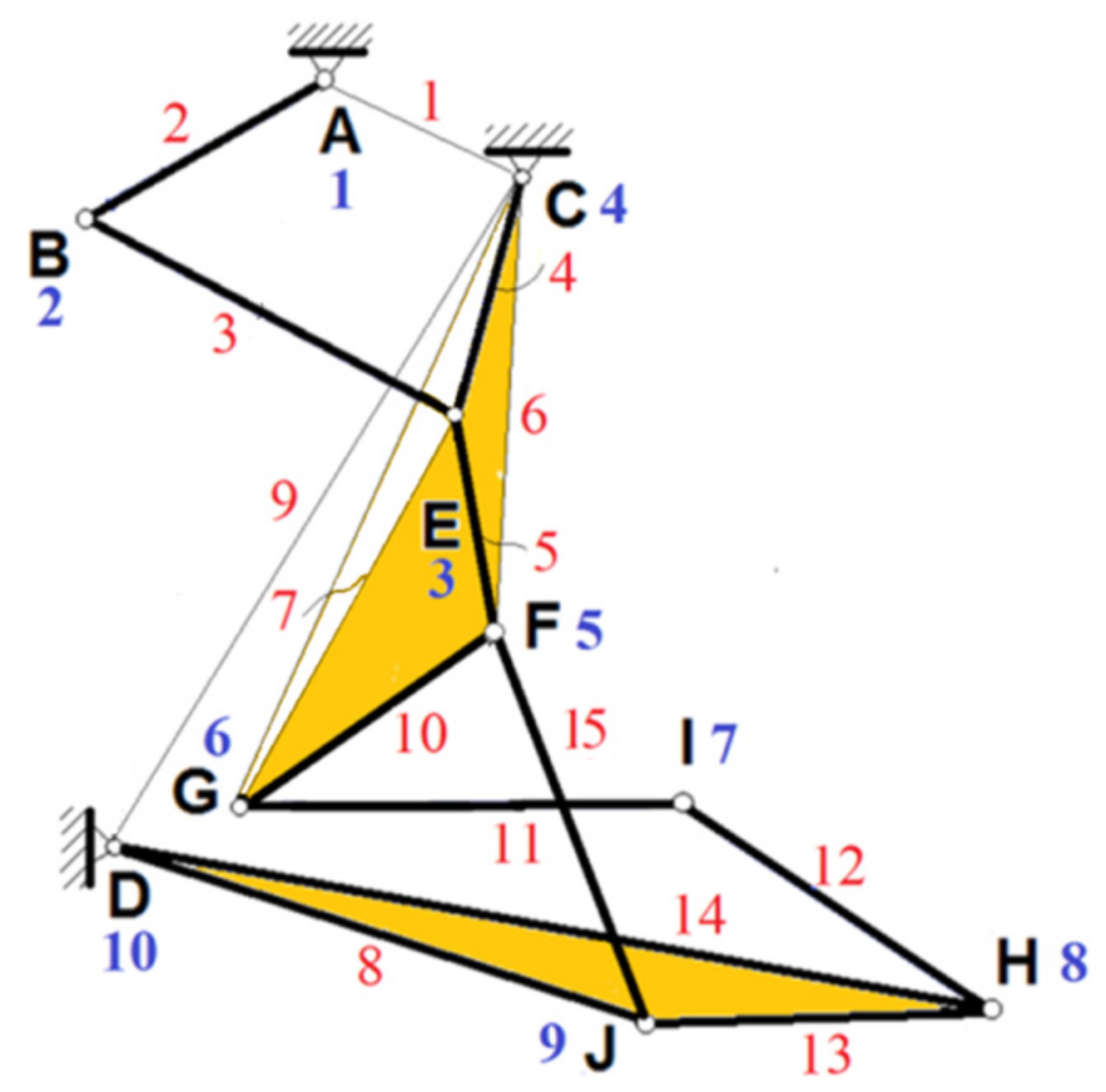
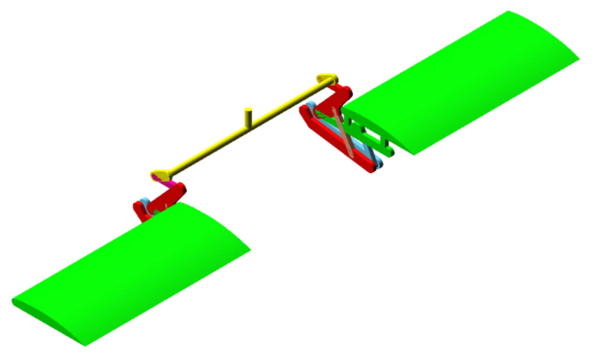
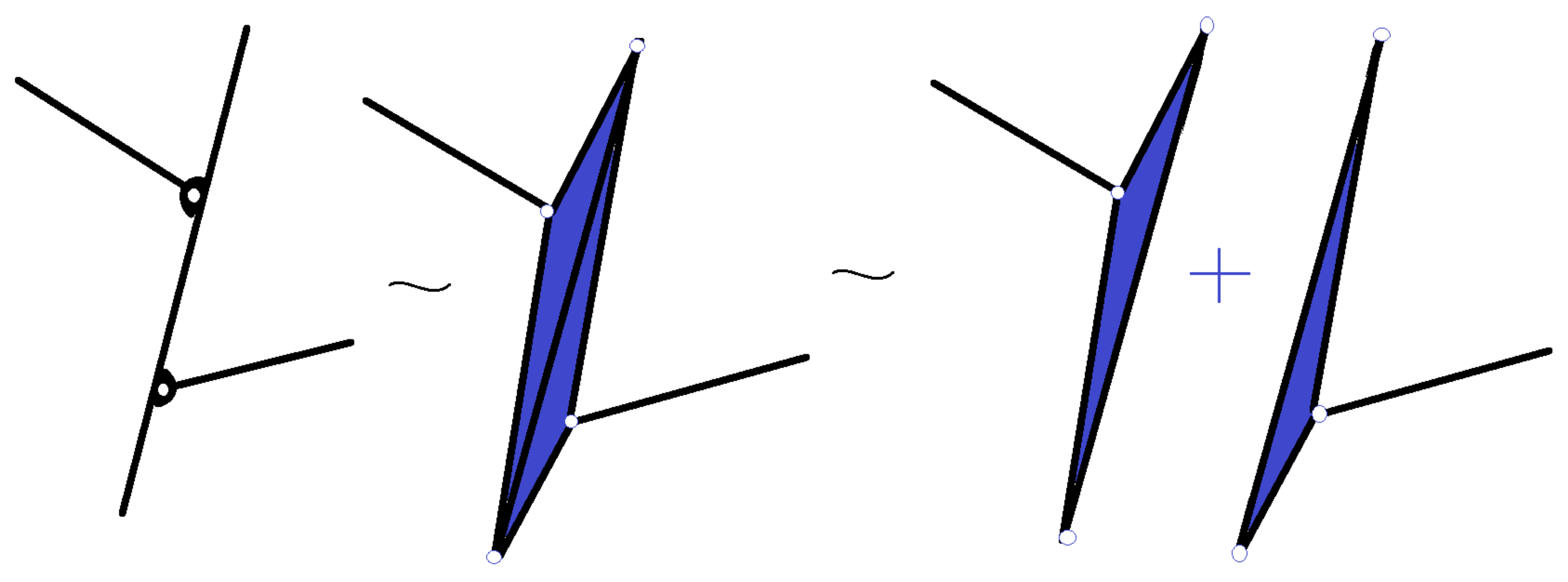
A planar mechanism with joints is considered (Figure 2) and designed to control the flaps of a light sports aircraft. The planar mechanism is made of bars connected by joints. There are ten joints and seven different bodies. The first stage is the construction of a planar mechanism, kinematic equivalent to the given mechanism, but composed only of bar-type elements with joints at both ends. The idea is to obtain an equivalent mechanism, but in which the mechanical behavior of the whole assembly has not changed (the characteristic points and the bars of this new mechanism move identically to those of the original mechanism). The following operations comply with these requirements:

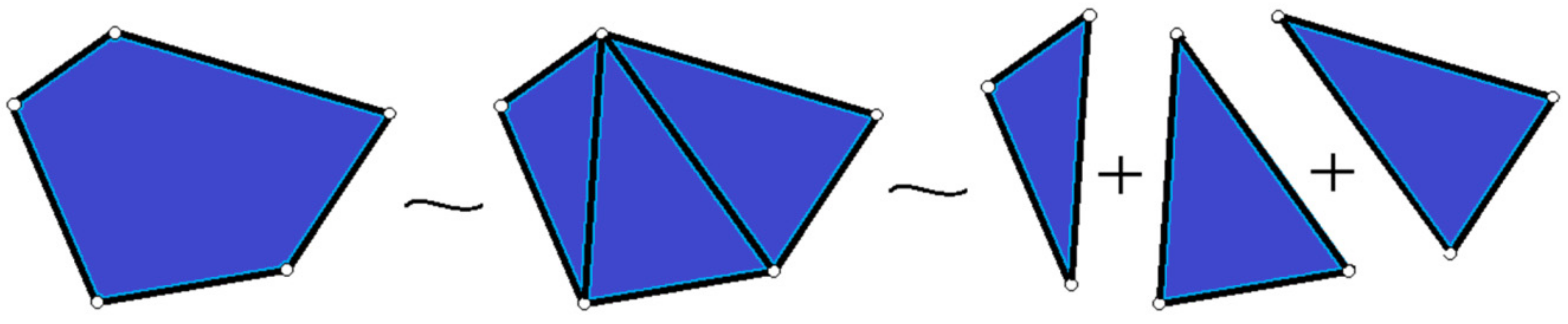
• Replace a plane two-dimensional element (Figure 3 and Figure 4) with the structure formed by bars connected by joints in a rigid connection, the number of bars that compose it being equal to the number of bars of the polygon defined by the plate element, to which are added all the diagonals starting from the same peak, regardless of choice. In this way a rigid flat plate is replaced with rigidly connected bars. Figure 3 shows how a polygon can be replaced with triangles, with every triangle made of three bars. Always, three bars are tied at the ends, between them, through the joints, constitutes a rigid structure. In Figure 4, a lever with multiple joints is replaced with triangles.
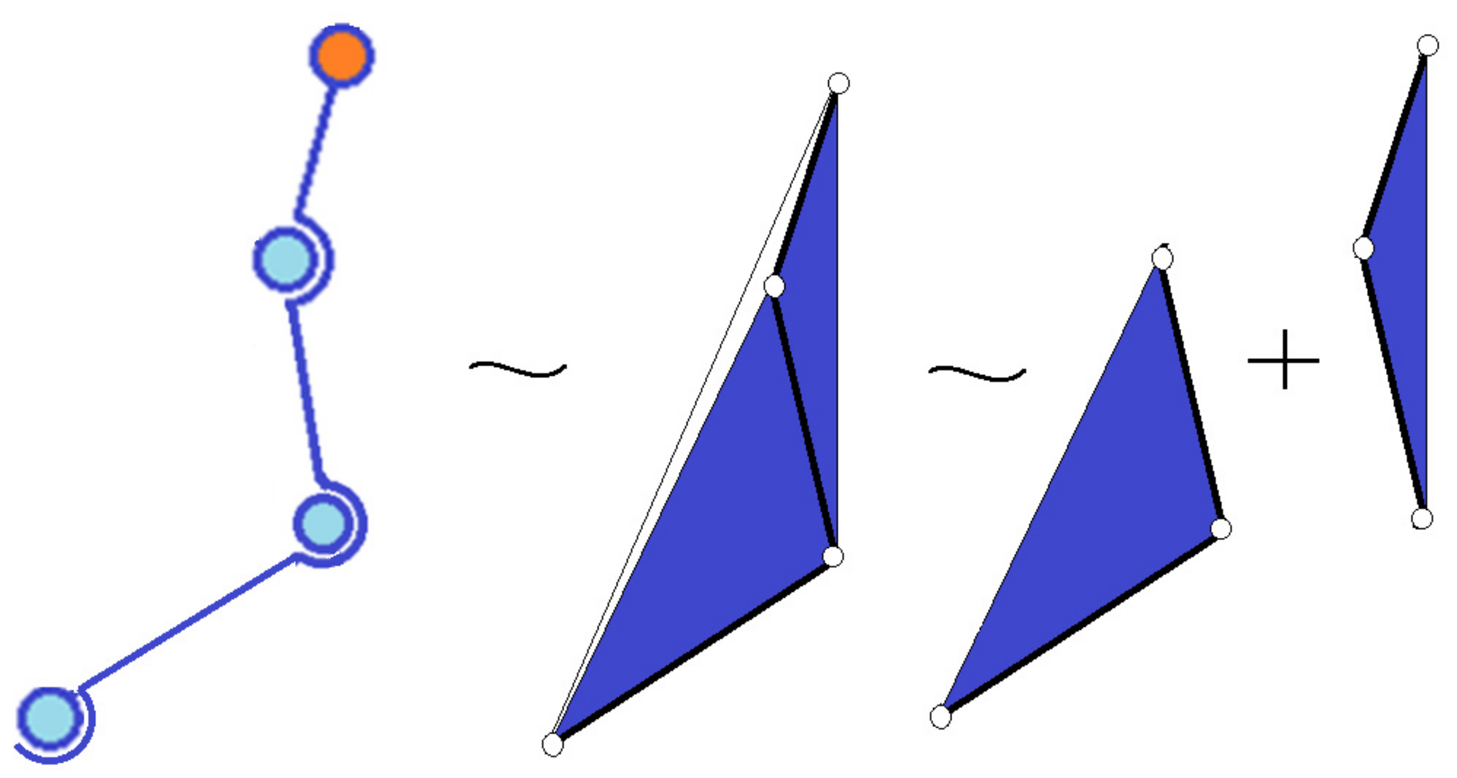
• A linear element with several joints is considered to be a plate (with a polygonal shape) with joints at the corner (in Figure 5, triangles). An example is presented in Figure 5. If three joints are situated on a line, the situation is equivalent to a triangle, having two angles zero and the third 180°. In such a way, the particular and degenerate cases are considered.
• The points making the connection with the ground (fixed element) are joined by bar-type elements that close a polygon (Figure 6), and then one of these elements is eliminated (it results from the vector sum, with changed sign of all the others). The elements obtained are considered to be elements with known motion, having velocities and angular accelerations of zero. Figure 6 represents the mechanism equivalent, from a kinematic point of view, to the mechanism in Figure 2. In obtaining this scheme, the properties presented above were used (Figure 3, Figure 4 and Figure 5).

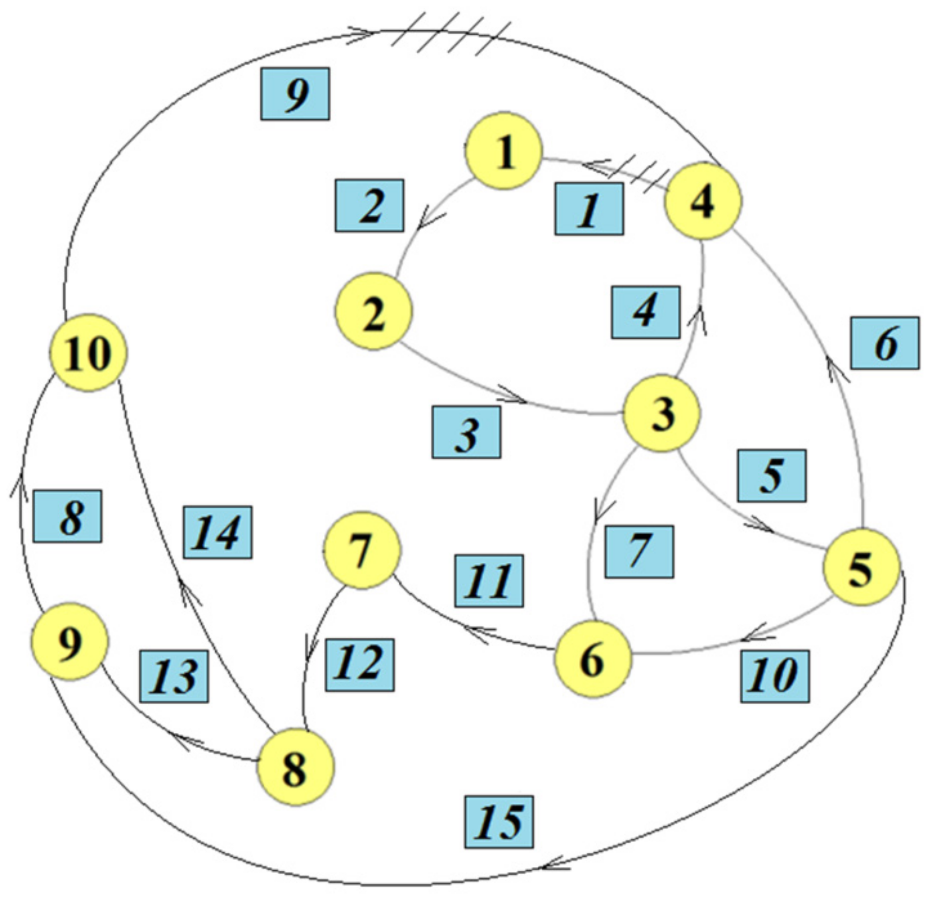
In this way, a mechanism is obtained that is kinematic equivalent to the initial mechanism, but which consists only of bars. Considering this new mechanism obtained by the previous operations, a graph is associated with the edges corresponding to the bar elements and the vertices corresponding to the joints [21]. Attaching to each bar a vector with the end in one joint and the top in the other and taking for each edge the direction of travel given by the direction of the vector thus constructed, the oriented graph from Figure 6 is obtained. Therefore, the topological description of the mechanism can be simplified. The equivalence method, described above, allows one to obtain, very easily, the graph associated with the planar mechanism.

In this way, a kinematic mechanism equivalent to the initial one will be obtained, but composed only of bars. This equivalent mechanism keeps the functionality and geometry of the initial mechanism, the input and output sizes are the same but allows the algorithmization of the kinematic analysis process. By applying these considerations to the mechanism presented in Figure 1, the mechanism from Figure 6 with the associated graph presented in Figure 7 is obtained. For the planar mechanism studied in the paper, the matrix of incidence is:

$$\begin{array}{cc}\hfill & node\setminus branch\hfill \\ \hfill & \begin{array}{ccccccccccccccc}1& 2& 3& 4& 5& 6& 7& 8& 9& 10& 11& 12& 13& 14& 15\end{array}\hfill \\ \hfill & \left[A\right]=\begin{array}{c}1\\ 2\\ 3\\ 4\\ 5\\ 6\\ 7\\ 8\\ 9\\ 10\end{array}\left[\begin{array}{ccccccccccccccc}-1& 1& 0& 0& 0& 0& 0& 0& 0& 0& 0& 0& 0& 0& 0\\ 0& -1& 1& 0& 0& 0& 0& 0& 0& 0& 0& 0& 0& 0& 0\\ 0& 0& -1& 1& 1& 0& 1& 0& 0& 0& 0& 0& 0& 0& 0\\ 1& 0& 0& -1& 0& -1& 0& 0& -1& 0& 0& 0& 0& 0& 0\\ 0& 0& 0& 0& -1& 1& 0& 0& 0& 1& 0& 0& 0& 0& 1\\ 0& 0& 0& 0& 0& 0& -1& 0& 0& -1& 1& 0& 0& 0& 0\\ 0& 0& 0& 0& 0& 0& 0& 0& 0& 0& -1& 1& 0& 0& 0\\ 0& 0& 0& 0& 0& 0& 0& 0& 0& 0& 0& -1& 1& 1& 0\\ 0& 0& 0& 0& 0& 0& 0& 1& 0& 0& 0& 0& -1& 0& -1\\ 0& 0& 0& 0& 0& 0& 0& -1& 1& 0& 0& 0& 0& -1& 0\end{array}\right]\hfill \end{array}$$

(9)

The matrix ${\left[A\right]}_a$ of rank r obtained by suppressing in ${\left[A\right]}_a$ line is called the reduced incidence matrix:

$$\begin{array}{cc}\hfill & node\setminus branch\hfill \\ \hfill & \begin{array}{ccccccccccccccc}1& 2& 3& 4& 5& 6& 7& 8& 9& 10& 11& 12& 13& 14& 15\end{array}\hfill \\ \hfill & {\left[A\right]}_a=\begin{array}{c}1\\ 2\\ 3\\ 4\\ 5\\ 6\\ 7\\ 8\\ 9\end{array}\left[\begin{array}{ccccccccccccccc}-1& 1& 0& 0& 0& 0& 0& 0& 0& 0& 0& 0& 0& 0& 0\\ 0& -1& 1& 0& 0& 0& 0& 0& 0& 0& 0& 0& 0& 0& 0\\ 0& 0& -1& 1& 1& 0& 1& 0& 0& 0& 0& 0& 0& 0& 0\\ 1& 0& 0& -1& 0& -1& 0& 0& 1& 0& 0& 0& 0& 0& 0\\ 0& 0& 0& 0& -1& 1& 0& 0& 0& 1& 0& 0& 0& 0& 1\\ 0& 0& 0& 0& 0& 0& -1& 0& 0& -1& 1& 0& 0& 0& 0\\ 0& 0& 0& 0& 0& 0& 0& 0& 0& 0& -1& 1& 0& 0& 0\\ 0& 0& 0& 0& 0& 0& 0& 0& 0& 0& 0& -1& 1& 1& 0\\ 0& 0& 0& 0& 0& 0& 0& 1& 0& 0& 0& 0& -1& 0& -1\end{array}\right]\hfill \end{array}$$

(10)

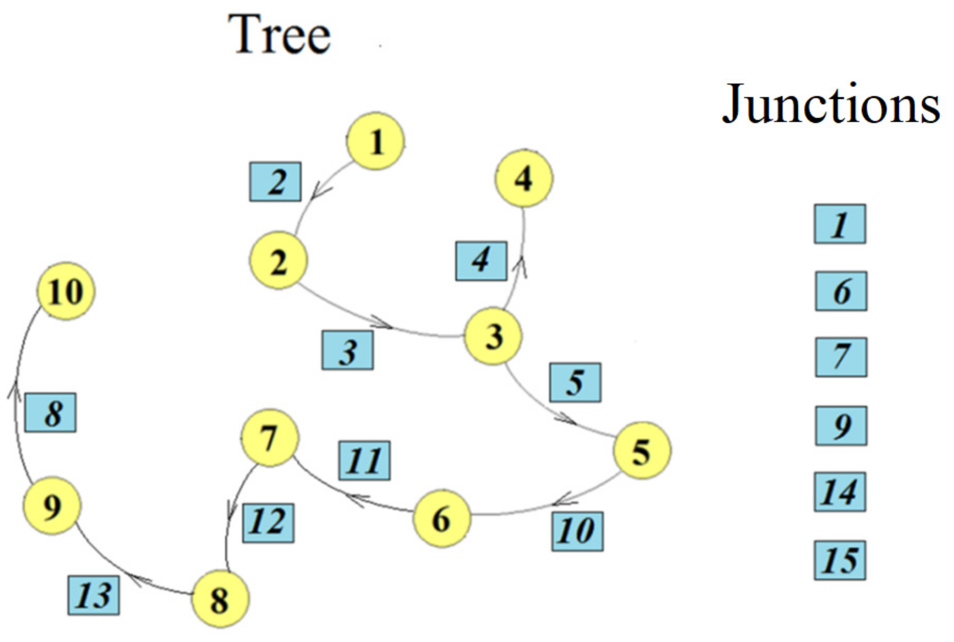
We can choose a tree of this graph (Figure 8). The tree is chosen using the considerations made in Section 2.1, regarding the description of the graphs. Selecting a tree in the presented graph allows a reordering and partitioning of ${\left[A\right]}_a$, it obtains the reduced incidence matrix under the form (only edges that are found in the chosen tree are entered in this matrix):

$${\left[A\right]}_a=[\left[A_t\right]\hspace{0.17em}⋮\hspace{0.17em}\left[A_l\right]\hspace{0.17em}]$$

(11)

so that the columns of $\left[A_t\right]$ correspond to the branches of the tree and the columns of $\left[A_l\right]$ to the junctions. For our mechanism the reordered matrix is:

$$\begin{array}{cc}\hfill & node\setminus branch\hfill \\ \hfill & \begin{array}{ccccccccccccccc}2& 3& 4& 5& 8& 10& 11& 12& 13& 1& 6& 7& 9& 14& 15\end{array}\hfill \\ \hfill & {\left[A\right]}_{areord}=\begin{array}{c}1\\ 2\\ 3\\ 4\\ 5\\ 6\\ 7\\ 8\\ 9\end{array}\left[\begin{array}{ccccccccccccccc}1& 0& 0& 0& 0& 0& 0& 0& 0& -1& 0& 0& 0& 0& -1\\ -1& 1& 0& 0& 0& 0& 0& 0& 0& 0& 0& 0& 0& 0& 0\\ 0& -1& 1& 1& 0& 0& 0& 0& 0& 0& 0& 1& 0& 0& 0\\ 0& 0& -1& 0& 0& 0& 0& 0& 0& 1& -1& 0& -1& 0& 0\\ 0& 0& 0& -1& 0& 1& 0& 0& 0& 0& 1& 0& 0& 0& 0\\ 0& 0& 0& 0& 0& -1& 1& 0& 0& 0& 0& -1& 0& 0& 0\\ 0& 0& 0& 0& 0& 0& -1& 1& 0& 0& 0& 0& 0& 0& 0\\ 0& 0& 0& 0& 0& 0& 0& -1& 1& 0& 0& 0& 0& 1& 0\\ 0& 0& 0& 0& 1& 0& 0& 0& -1& 0& 0& 0& 0& 0& 0\end{array}\right]\hfill \end{array}$$

(12)

where:

$$\begin{array}{l}\hspace{1em}\hspace{1em}node\backslash branch\\ \hspace{1em}\hspace{1em}\hspace{1em}\hspace{1em}\hspace{1em}\begin{array}{ccccccccc}\hspace{0.17em}2& \hspace{0.33em}\hspace{0.17em}3& \hspace{0.33em}\hspace{0.33em}4& \hspace{0.33em}\hspace{0.17em}5& 8& \hspace{0.33em}10& 11& \hspace{0.17em}12& 13\end{array}\\ {\left[A\right]}_t=\hspace{1em}\hspace{1em}\hspace{0.33em}\begin{array}{c}1\\ 2\\ 3\\ 4\\ 5\\ 6\\ 7\\ 8\\ 9\end{array}\left[\begin{array}{ccccccccc}1& 0& 0& 0& 0& 0& 0& 0& 0\\ -1& 1& 0& 0& 0& 0& 0& 0& 0\\ 0& -1& 1& 1& 0& 0& 0& 0& 0\\ 0& 0& -1& 0& 0& 0& 0& 0& 0\\ 0& 0& 0& -1& 0& 1& 0& 0& 0\\ 0& 0& 0& 0& 0& -1& 1& 0& 0\\ 0& 0& 0& 0& 0& 0& -1& 1& 0\\ 0& 0& 0& 0& 0& 0& 0& -1& 1\\ 0& 0& 0& 0& 1& 0& 0& 0& -1\end{array}\right]\end{array}$$

(13)

and:

$$\begin{array}{l}\hspace{1em}\hspace{1em}node\backslash branch\\ \hspace{1em}\hspace{1em}\hspace{1em}\hspace{1em}\hspace{1em}\hspace{1em}\begin{array}{ccccccc}1& 6& 7& 9& 14& 15& \end{array}\\ {\left[A\right]}_l=\hspace{1em}\hspace{1em}\hspace{0.33em}\begin{array}{c}1\\ 2\\ 3\\ 4\\ 5\\ 6\\ 7\\ 8\\ 9\end{array}\left[\begin{array}{cccccc}-1& 0& 0& 0& 0& -1\\ 0& 0& 0& 0& 0& 0\\ 0& 0& 1& 0& 0& 0\\ 1& -1& 0& -1& 0& 0\\ 0& 1& 0& 0& 0& 0\\ 0& 0& -1& 0& 0& 0\\ 0& 0& 0& 0& 0& 0\\ 0& 0& 0& 0& 1& 0\\ 0& 0& 0& 0& 0& 0\end{array}\right]\end{array}$$

(14)

Now, the fundamental loop matrix can be written as:

$$\begin{array}{c}{\left[B\right]}_f=[{[-{\left[A\right]}_t^{-1}{\left[A\right]}_l]}^T⋮\left[E\right]]=\\ \begin{array}{cc}\hfill & cycle\setminus branch2345\hspace{0.17em}\hspace{0.17em}81011121316791415\hfill \\ \hfill & \begin{array}{c}1\\ 2\\ 3\\ 4\\ 5\\ 6\end{array}\left[\begin{array}{ccccccccccccccc}1& 1& 1& 0& 0& 0& 0& 0& 0& 1& 0& 0& 0& 0& 0\\ 0& 0& -1& 1& 0& 0& 0& 0& 0& 0& 1& 0& 0& 0& 0\\ 0& 0& 0& -1& 0& -1& 0& 0& 0& 0& 0& 1& 0& 0& 0\\ 0& 0& -1& 1& 1& 1& 1& 1& 1& 0& 0& 0& 1& 0& 0\\ 0& 0& 0& 0& -1& 0& 0& 0& -1& 0& 0& 0& 0& 1& 0\\ 0& 0& 0& 0& 0& -1& -1& -1& -1& 0& 0& 0& 0& 0& 1\end{array}\right]\hfill \end{array}\end{array}$$

(15)

which allows the determination of the matrix of the fundamental loops (one of them) if the incident matrix has been constructed and a tree [21] has been identified. This matrix is not unique, it depends on the tree of the graph chosen. Thus, there can be several matrices of the fundamental loops, but with the same dimensions of the matrix. Whatever form is used, the end results is the same. Obviously, matrices that have a small number of elements are preferred.

We perform a partition of ${\left[B\right]}_f$, ${\left[B\right]}_f=[{\left[B\right]}_{fn}⋮{\left[B\right]}_{fc}]$ made after a rearrangement of the columns of ${\left[B\right]}_f$, so that the matrix ${\left[B\right]}_f$ corresponds to the elements of the first class, and ${\left[B\right]}_{fc}$ to the elements of the second class.

$$\begin{array}{cc}\hfill & cycle\setminus branch\hspace{0.33em}345678101112131415129\hfill \\ \hfill & {\left[B\right]}_{freord}=\begin{array}{c}1\\ 2\\ 3\\ 4\\ 5\\ 6\end{array}\left[\begin{array}{ccccccccccccccc}1& 1& 0& 0& 0& 0& 0& 0& 0& 0& 0& 0& 1& 1& 0\\ 0& -1& 1& 1& 0& 0& 0& 0& 0& 0& 0& 0& 0& 0& 0\\ 0& 0& -1& 0& 1& 0& -1& 0& 0& 0& 0& 0& 0& 0& 0\\ 0& -1& 1& 0& 0& 1& 1& 1& 1& 1& 0& 0& 0& 0& 1\\ 0& 0& 0& 0& 0& -1& 0& 0& 0& -1& 1& 0& 0& 0& 0\\ 0& 0& 0& 0& 0& 0& -1& -1& -1& -1& 0& 1& 0& 0& 0\end{array}\right]\hfill \end{array}$$

(16)

$$\begin{array}{l}cycle\backslash branch\hspace{0.33em}\hspace{0.33em}\hspace{0.33em}\hspace{0.33em}\hspace{0.33em}\hspace{0.33em}3\hspace{1em}\hspace{0.17em}\hspace{0.17em}4\hspace{1em}\hspace{0.17em}\hspace{0.33em}5\hspace{1em}\hspace{0.17em}6\hspace{1em}7\hspace{1em}\hspace{0.33em}8\hspace{1em}\hspace{0.33em}10\hspace{0.17em}\hspace{0.33em}\hspace{0.33em}11\hspace{0.33em}\hspace{0.33em}12\hspace{0.33em}\hspace{0.33em}13\hspace{0.17em}\hspace{0.33em}14\hspace{0.33em}\hspace{0.17em}\hspace{0.17em}15\hspace{1em}\\ {\left[B\right]}_{fn}=\hspace{1em}\hspace{0.33em}\hspace{1em}\begin{array}{c}1\\ 2\\ 3\\ 4\\ 5\\ 6\end{array}\hspace{1em}\left[\begin{array}{cccccccccccc}1& 1& 0& 0& 0& 0& 0& 0& 0& 0& 0& 0\\ 0& -1& 1& 1& 0& 0& 0& 0& 0& 0& 0& 0\\ 0& 0& -1& 0& 1& 0& -1& 0& 0& 0& 0& 0\\ 0& -1& 1& 0& 0& 1& 1& 1& 1& 1& 0& 0\\ 0& 0& 0& 0& 0& -1& 0& 0& 0& -1& 1& 0\\ 0& 0& 0& 0& 0& 0& -1& -1& -1& -1& 0& 1\end{array}\right]\end{array}$$

(17)

$$\begin{array}{l}cycle\backslash branch\hspace{0.33em}\hspace{0.33em}\hspace{0.33em}\hspace{0.33em}1\hspace{1em}\hspace{0.17em}2\hspace{1em}9\hspace{1em}\\ {\left[B\right]}_{fc}=\hspace{1em}\hspace{0.33em}\hspace{1em}\begin{array}{c}1\\ 2\\ 3\\ 4\\ 5\\ 6\end{array}\hspace{1em}\left[\begin{array}{ccc}1& 1& 0\\ 0& 0& 0\\ 0& 0& 0\\ 0& 0& 1\\ 0& 0& 0\\ 0& 1& 0\end{array}\right]\end{array}$$

(18)

We construct the diagonal matrices of size s, which have on the diagonal, the following information about the bar-type elements, in the order in which they are in the matrix of the fundamental loops, rearranged lengths, grouped in the matrix $\left[L\right]$:

$$\left[L\right]=\left[\begin{array}{ccc}{L}_n& ⋮& 0\\ \cdots & ⋮& \cdots \\ 0& ⋮& L_c\end{array}\right]$$

(19)

where:

$$\left[L_n\right]=\left[\begin{array}{cccccccc}{l}_3& & & & & & & \\ & l_4& & & & & & \\ & & l_5& & & 0& & \\ & & & \ddots & & & & \\ & & & & \ddots & & & \\ & & 0& & & l_{13}& & \\ & & & & & & l_{14}& \\ & & & & & & & l_{15}\end{array}\right] ,$$

(20)

and:

$$\left[L_c\right]=\left[\begin{array}{ccc}{l}_1& 0& 0\\ 0& l_2& 0\\ 0& 0& l_9\end{array}\right] ;$$

(21)

-

the cosines of the angles made by the bars with the horizontal axis;

$$\left[C\right]=\left[\begin{array}{ccc}{C}_n& ⋮& 0\\ \cdots & ⋮& \cdots \\ 0& ⋮& C_c\end{array}\right] ;$$

(22)

where:

$$\left[C_n\right]=\left[\begin{array}{cccccccc}\cos {\theta }_3& & & & & & & \\ & \cos {\theta }_4& & & & & & \\ & & \cos {\theta }_5& & & 0& & \\ & & & \ddots & & & & \\ & & & & \ddots & & & \\ & & 0& & & \cos {\theta }_{13}& & \\ & & & & & & \cos {\theta }_{14}& \\ & & & & & & & \cos {\theta }_{15}\end{array}\right] ,$$

(23)

and:

$$\left[C_c\right]=\left[\begin{array}{ccc}\cos {\theta }_1& 0& 0\\ 0& \cos {\theta }_2& 0\\ 0& 0& \cos {\theta }_9\end{array}\right] ;$$

(24)

-

the sines of the angles made by the bars with the horizontal axis;

$$\left[S\right]=\left[\begin{array}{ccc}{S}_n& ⋮& 0\\ \cdots & ⋮& \cdots \\ 0& ⋮& S_c\end{array}\right] ,$$

(25)

where:

$$\left[S_n\right]=\left[\begin{array}{cccccccc}\sin {\theta }_3& & & & & & & \\ & \sin {\theta }_4& & & & & & \\ & & \sin {\theta }_5& & & 0& & \\ & & & \ddots & & & & \\ & & & & \ddots & & & \\ & & 0& & & \sin {\theta }_{13}& & \\ & & & & & & \sin {\theta }_{14}& \\ & & & & & & & \sin {\theta }_{15}\end{array}\right] ;$$

(26)

and:

$$\left[S_c\right]=\left[\begin{array}{ccc}\sin {\theta }_1& 0& 0\\ 0& \sin {\theta }_2& 0\\ 0& 0& \sin {\theta }_9\end{array}\right]$$

(27)

We define the column vectors with size s:

$$\left\{\omega \right\}=\left\{\begin{array}{c}{\omega }_n\\ \cdots \\ {\omega }_c\end{array}\right\}=\left\{\begin{array}{c}{\omega }_3\\ {\omega }_4\\ ⋮\\ ⋮\\ {\omega }_{15}\\ \cdots \\ {\omega }_1\\ {\omega }_2\\ {\omega }_9\end{array}\right\}\hspace{1em};\hspace{1em}\left\{{\omega }^2\right\}=\left\{\begin{array}{c}{\omega }_n^2\\ \cdots \\ {\omega }_c^2\end{array}\right\}=\left\{\begin{array}{c}{\omega }_3^2\\ {\omega }_4^2\\ ⋮\\ ⋮\\ {\omega }_{15}^2\\ \cdots \\ {\omega }_1^2\\ {\omega }_2^2\\ {\omega }_9^2\end{array}\right\}\hspace{1em};\hspace{1em}\left\{\epsilon \right\}=\left\{\begin{array}{c}{\epsilon }_n\\ \cdots \\ {\epsilon }_c\end{array}\right\}=\left\{\begin{array}{c}{\epsilon }_3\\ {\epsilon }_4\\ ⋮\\ ⋮\\ {\epsilon }_{15}\\ \cdots \\ {\epsilon }_1\\ {\epsilon }_2\\ {\epsilon }_9\end{array}\right\} ,$$

(28)

where the partitions were made following the division of the elements into the two classes:

• Elements whose movement are not know, but we want to determine;
• Elements with known and fixed motion.

The following notations have been used:

$l_i$—the length of the numbered element i;

${\theta }_i$—the angle made by the vector ${\overline{l}}_i$ with the axis Ox of the global coordinate system xOy;

${\overline{\omega }}_i$—the angular velocity of the element numbered with i;

${\overline{\epsilon }}_i$—the angular acceleration of the element i.

Using the results obtained by graph theory, we establish the results that offer an algorithm to determine the field of the velocities and acceleration of the studied mechanism.

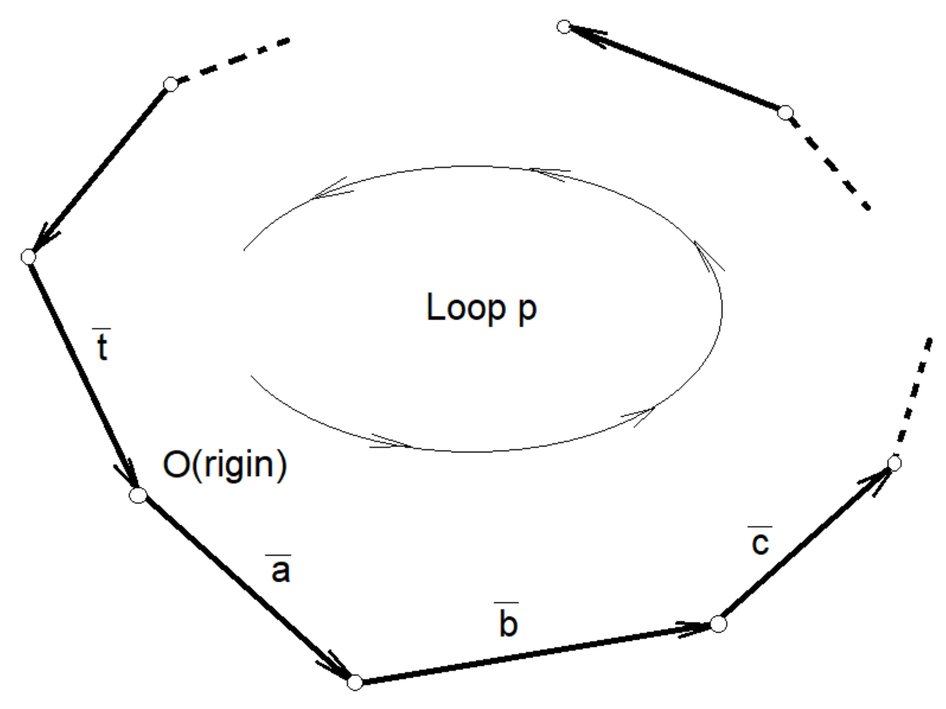
Let p be the loop of the system of fundamental loops (independent cycles) consisting of the elements a, b, c, …, t (Figure 9). The vector closure equation:

$${\overline{l}}_a+{\overline{l}}_b+{\overline{l}}_c+\dots \hspace{1em}\dots +{\overline{l}}_t=0 ,$$

(29)

offers the projection equations:

$$\begin{array}{c}{l}_{a}cos{\theta }_a+l_{b}cos{\theta }_b+l_{c}cos{\theta }_c+\dots \dots +l_{t}cos{\theta }_t=0;\\ l_{a}sin{\theta }_a+l_{b}sin{\theta }_b+l_{c}sin{\theta }_c+\dots \dots +l_{t}sin{\theta }_t=0.\end{array}$$

(30)

Differentiating in relation to time, we obtain:

$$\begin{array}{c}-{\omega }_a{l}_{a}sin{\theta }_a-{\omega }_b{l}_{b}sin{\theta }_b-{\omega }_c{l}_{c}sin{\theta }_c+\dots \dots -{\omega }_t{l}_{t}sin{\theta }_t=0;\\ {\omega }_a{l}_{a}cos{\theta }_a+{\omega }_b{l}_{b}cos{\theta }_b+{\omega }_c{l}_{c}cos{\theta }_c+\dots +{\omega }_t{l}_{t}cos{\theta }_t=0.\end{array}$$

(31)

If noted:

$$\begin{array}{l}\begin{array}{cccccccccccccccccc}\hspace{1em}& 1& 2& \dots & & \dots & a& \dots & & \dots & b& \dots & & \dots & t& \dots & \hspace{1em}\dots & s\end{array}\\ \left[B_p\right]=\left[\begin{array}{cccccccccccccccccc}\hspace{0.33em}\hspace{0.33em}0& \hspace{0.33em}\hspace{0.33em}0& \hspace{0.33em}\hspace{0.33em}0& & \hspace{1em}0& \hspace{1em}1& \hspace{1em}\hspace{0.33em}0& \hspace{0.33em}& \hspace{0.33em}\hspace{0.33em}\hspace{0.17em}\hspace{0.17em}0& \hspace{0.17em}\hspace{0.17em}\hspace{0.17em}1& \hspace{0.17em}0& \hspace{1em}& \hspace{1em}\hspace{0.17em}0& \hspace{0.33em}\hspace{0.17em}1& \hspace{0.33em}\hspace{0.17em}0& & \hspace{0.17em}0& 0\end{array}\right]\end{array}$$

(32)

the system (31) allows the matrix writing:

$$\left\{\begin{array}{l}-\left[B_p\right]\left[L\right]\left[S\right]\left\{\omega \right\}=0\\ \left[B_p\right]\left[L\right]\left[C\right]\left\{\omega \right\}=0\end{array}\right.$$

(33)

It is observed that $\left[B_p\right]$ is considered to be the p line in the matrix of the fundamental loops $\left[B_f\right]$. Repeating the procedure described for each fundamental loop, we obtain, by assembling all Equation (33):

$$\left\{\begin{array}{l}-\left[B_f\right]\left[L\right]\left[S\right]\left\{\omega \right\}=0\\ \left[B_f\right]\left[L\right]\left[C\right]\left\{\omega \right\}=0\end{array}\right.$$

(34)

Considering the notations made at the beginning of this paragraph and performing the partitioned matrix products, we can write Equation (34) in the form:

$$\left[\begin{array}{cc}-\left[B_{fn}\right]\left[L_n\right]\left[S_n\right]& -\left[B_{fc}\right]\left[L_c\right]\left[S_c\right]\\ \left[B_{fn}\right]\left[L_n\right]\left[C_n\right]& \left[B_{fc}\right]\left[L_c\right]\left[C_c\right]\end{array}\right]\left\{\begin{array}{c}{\omega }_n\\ \cdots \\ {\omega }_c\end{array}\right\}=0$$

(35)

Differentiating Equation (31), the result is:

$$\begin{array}{c}-{\omega }_a^2{l}_a\cos {\theta }_a-{\omega }_b^2{l}_b\cos {\theta }_b-{\omega }_c^2{l}_c\cos {\theta }_c+\dots \hspace{1em}\dots -{\omega }_t^2{l}_t\cos {\theta }_t\\ -{\epsilon }_a{l}_a\sin {\theta }_a-{\epsilon }_b{l}_b\sin {\theta }_b-{\epsilon }_c{l}_c\sin {\theta }_c+\dots \hspace{1em}\dots -{\epsilon }_t{l}_t\sin {\theta }_t=0\\ -{\omega }_a^2{l}_a\sin {\theta }_a-{\omega }_b^2{l}_b\sin {\theta }_b-{\omega }_c^2{l}_c\sin {\theta }_c+\dots \hspace{1em}\dots -{\omega }_t^2{l}_t\sin {\theta }_t\\ +{\epsilon }_a{l}_a\cos {\theta }_a+{\epsilon }_b{l}_b\cos {\theta }_b+{\epsilon }_c{l}_c\cos {\theta }_c+\dots \hspace{1em}\dots +{\epsilon }_t{l}_t\cos {\theta }_t=0\end{array}$$

(36)

Using the previously introduced notations we obtain:

$$\left\{\begin{array}{l}-\left[B_p\right]\left[L\right]\left[C\right]\left\{{\omega }^2\right\}-\left[B_p\right]\left[L\right]\left[S\right]\left\{\epsilon \right\}=0\\ -\left[B_p\right]\left[L\right]\left[S\right]\left\{\omega \right\}+\left[B_p\right]\left[L\right]\left[C\right]\left\{\epsilon \right\}=0\end{array}\right.$$

(37)

By writing the equations for all the fundamental loops, we obtain, after assembly:

$$\left\{\begin{array}{l}-\left[B_f\right]\left[L\right]\left[C\right]\left\{{\omega }^2\right\}-\left[B_f\right]\left[L\right]\left[S\right]\left\{\epsilon \right\}=0\\ -\left[B_f\right]\left[L\right]\left[S\right]\left\{\omega \right\}+\left[B_f\right]\left[L\right]\left[C\right]\left\{\epsilon \right\}=0\end{array}\right.$$

(38)

It follows, in the same way as for angular velocities, the relations:

$$-\left[\begin{array}{cc}-\left[B_{fn}\right]\left[L_n\right]\left[C_n\right]& -\left[B_{fc}\right]\left[L_c\right]\left[C_c\right]\\ \left[B_{fn}\right]\left[L_n\right]\left[S_n\right]& \left[B_{fc}\right]\left[L_c\right]\left[S_c\right]\end{array}\right]\left\{\begin{array}{c}{\omega }_n^2\\ \cdots \\ {\omega }_c^2\end{array}\right\}+\left[\begin{array}{cc}-\left[B_{fn}\right]\left[L_n\right]\left[S_n\right]& -\left[B_{fc}\right]\left[L_c\right]\left[S_c\right]\\ \left[B_{fn}\right]\left[L_n\right]\left[C_n\right]& \left[B_{fc}\right]\left[L_c\right]\left[C_c\right]\end{array}\right]\left\{\begin{array}{c}{\epsilon }_n\\ \cdots \\ {\epsilon }_c\end{array}\right\}=0$$

(39)

If noted:

$$\left[P_{sn}\right]=\left[B_{fn}\right]\left[L_n\right]\left[S_n\right]\hspace{1em};\hspace{1em}\left[P_{cn}\right]=\left[B_{fn}\right]\left[L_n\right]\left[C_n\right]\hspace{1em};\hspace{1em}\left[P_{sc}\right]=\left[B_{fc}\right]\left[L_c\right]\left[S_c\right]\hspace{1em};\hspace{1em}\left[P_{cc}\right]=\left[B_{fc}\right]\left[L_c\right]\left[C_c\right]$$

(40)

and:

$$\left[P_n\right]=\left[\begin{array}{c}-P_{sn}\\ P_{cn}\end{array}\right]\hspace{1em};\hspace{1em}\left[P_c\right]=\left[\begin{array}{c}-P_{sc}\\ P_{cc}\end{array}\right]\hspace{1em};\hspace{1em}\left[Q_n\right]=\left[\begin{array}{c}{P}_{cn}\\ P_{sn}\end{array}\right]\hspace{1em};\hspace{1em}\left[Q_c\right]=\left[\begin{array}{c}{P}_{cc}\\ P_{sc}\end{array}\right]\hspace{1em}$$

(41)

Relationships (35) and (39) become, respectively:

$$\left[\begin{array}{ccc}{P}_n& ⋮& P_c\end{array}\right]\left\{\begin{array}{c}{\omega }_n\\ \cdots \\ {\omega }_c\end{array}\right\}=0,$$

(42)

$$-\left[\begin{array}{ccc}{Q}_n& ⋮& Q_c\end{array}\right]\left\{\begin{array}{c}{\omega }_n^2\\ \cdots \\ {\omega }_c^2\end{array}\right\}+\left[\begin{array}{ccc}{P}_n& ⋮& P_c\end{array}\right]\left\{\begin{array}{c}{\epsilon }_n\\ \cdots \\ {\epsilon }_c\end{array}\right\}=0$$

(43)

Using the developments for Equations (42) and (43), we obtain:

$$\left[P_n\right]\left\{{\omega }_n\right\}+\left[P_c\right]\left\{{\omega }_c\right\}=0$$

(44)

and

$$-\left[Q_n\right]\left\{{\omega }_n^2\right\}-\left[Q_c\right]\left\{{\omega }_c^2\right\}+\left[P_n\right]\left\{{\epsilon }_n\right\}+\left[P_c\right]\left\{{\epsilon }_c\right\}=0$$

(45)

So, it is obtained, simply:

$$\left\{{\omega }_n\right\}=-{\left[P_n\right]}^{-1}\left[P_c\right]\left\{{\omega }_c\right\}$$

(46)

and:

$$\left\{{\epsilon }_n\right\}={\left[P_n\right]}^{-1}\left(-\left[P_c\right]\left\{{\epsilon }_c\right\}+\left[Q_n\right]\left\{{\omega }_n^2\right\}+\left[Q_c\right]\left\{{\omega }_c^2\right\}\right)$$

(47)

Thus, we can determine the angular velocities and angular accelerations of the bar-type elements whose motion we want to determine, depending on the angular velocities and accelerations of the elements whose motion we know.

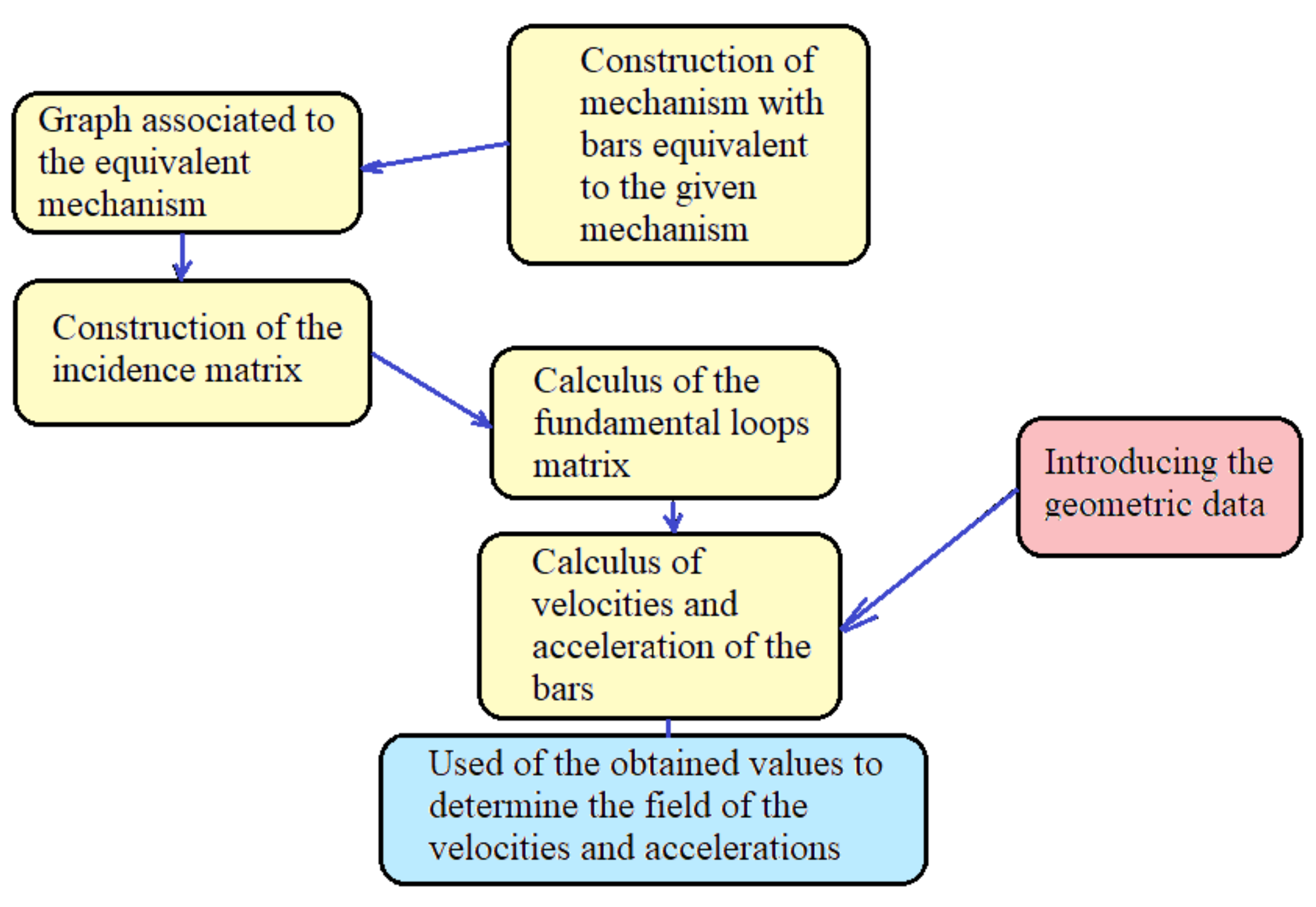
2.4. The Description of the Algorithm

On the basis of the considerations and constructions presented above, an algorithm can be proposed to allow the kinematic analysis of the studied mechanism. The necessary steps to be taken are:

• Construction of a mechanism composed of bars with joints, having the same mechanical behavior as the given mechanism. The plates that may exist in the flat mechanisms are replaced by bar systems, which ensure the rigidity of the structure thus obtained. Three interconnected bars always ensure a rigid behavior of the obtained structure. The way in which this construction is done is presented in Section 2.1.
• Composition of the graph associated with the given mechanism. This is done simply, considering the bars of the mechanism as edges and the joints as vertices.
• Writing the incidence matrix. This is the main stage of the analysis. The incidence matrix contains all the information regarding the structure of the analyzed mechanism.
• Calculation of the matrix of fundamental loops. This is done simply by applying the relationships previously presented in the paper. This identifies the main vector contours that allow us to analyze the kinematics and determine the unknowns.
• According to the analysis made in Equations (46) and (47), the angular velocities and accelerations of the bars that compose the mechanism are determined.
• If these sizes are known, the speeds and accelerations of any point of the mechanism can be determined, depending on the proposed design theme.

Considering this algorithm, an application is made to obtain the field of velocities and accelerations for a command mechanism of a light sport aircraft.

A schematic of the algorithm is shown in Figure 10.

3. Kinematic Analysis of the Control Mechanism

The technical problem solved by the flap control mechanism is improvement of the dynamic behavior of a light aircraft through the constructive form of the aircraft. The flap control mechanism allows steering angles greater than 40° required for takeoffs and landings over a short distance and a shorter time and increased load capacity, as well as the operation of the aircraft in critical flight conditions or when fuel economy is required, since the aircraft has the ability to glide in these situations, and conditions of low manufacturing costs [6,22,23,24,25,26,27]. The light aircraft proposed for the light sport aircraft category, is designed for sport and leisure aviation, with a maximum capacity of two seats and an aerodynamic shape that has curved flaps mounted on the wings without hinges for the flight board. However, the described algorithm can be applied at every planar mechanism. The light aircraft has a maximum take-off weight of 900 kg, a cruising speed of 450 km per hour, and the maximum flight ceiling is 5000 m. These data are informative, however, do not play a significant role in the required calculations. The challenge of designing a control mechanism for this type of aircraft is of great importance.

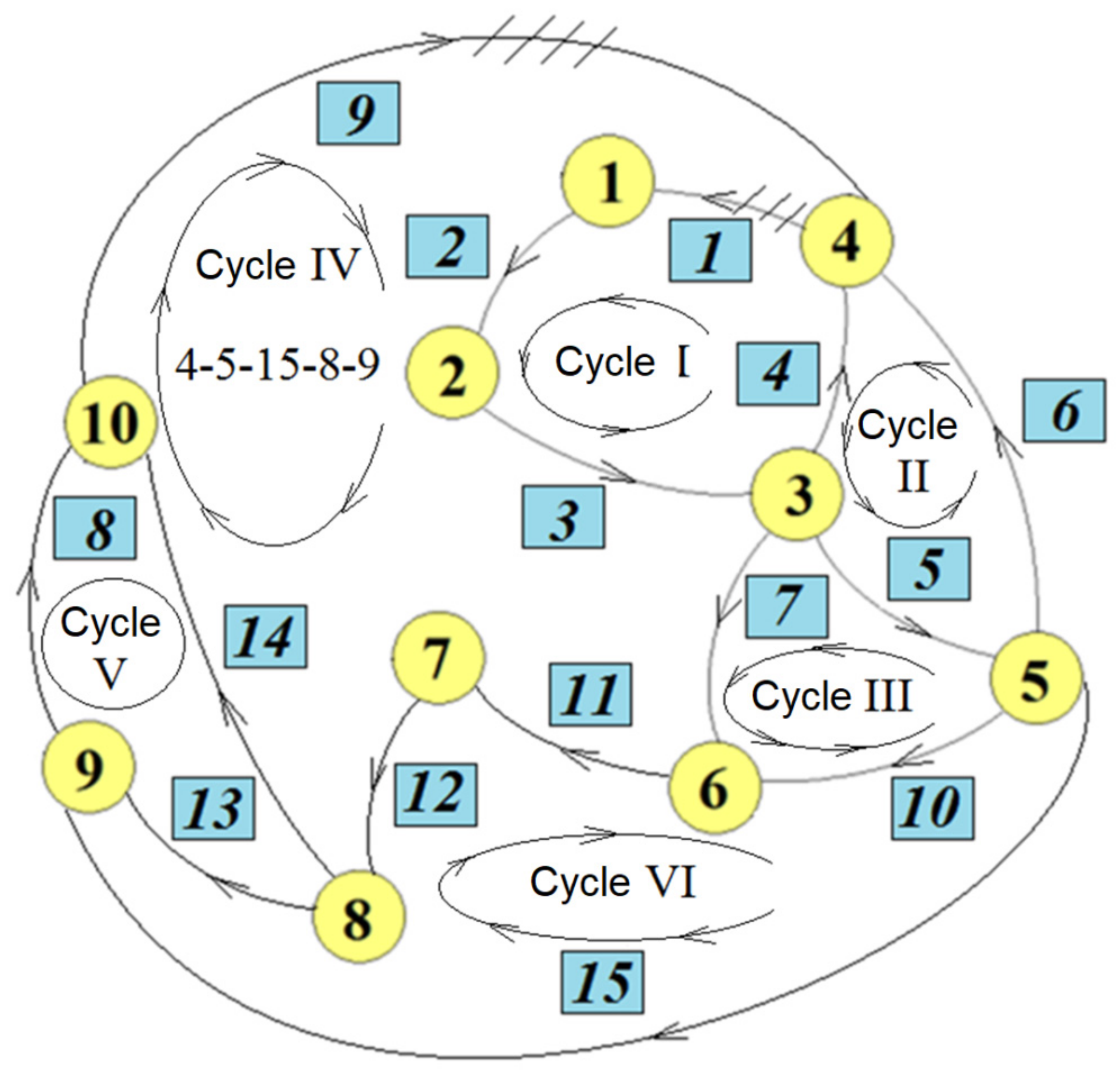
The kinematic analysis was performed for the mechanism presented in Figure 2 and Figure 11, with the kinematic sketch shown in Figure 6. For this mechanism, the associated graph was built (Figure 7), a tree was established (Figure 8), and then with its help, the fundamental loop matrix was built, partitioned according to elements with known motion or fixed and elements with unknown motion.

With Relation (15), the matrix of the fundamental loops is obtained. Each line of this matrix defines a fundamental loop. The number of loops that can be built in a graph is higher, but any loop can be obtained as a combination of fundamental loops. What matters in the description of the mechanism are the fundamental loops. In our application, we have six independent loops, defined by the six lines of the matrix of the fundamental loops. The equations for the six fundamental loops (Figure 12) are the following:

$$\begin{array}{l}{\overline{l}}_3+{\overline{l}}_4+{\overline{l}}_1+{\overline{l}}_2=0\hspace{1em};\\ -{\overline{l}}_4+{\overline{l}}_5+{\overline{l}}_6=0\hspace{1em};\\ -{\overline{l}}_5+l_7-{\overline{l}}_{10}=0\hspace{1em};\\ -{\overline{l}}_4+{\overline{l}}_5+{\overline{l}}_8+{\overline{l}}_{15}+{\overline{l}}_9=0\hspace{1em};\\ -{\overline{l}}_8-{\overline{l}}_{13}+{\overline{l}}_{14}=0\hspace{1em};\\ -{\overline{l}}_{10}-{\overline{l}}_{11}-{\overline{l}}_{12}-{\overline{l}}_{13}+{\overline{l}}_{15}=0\hspace{1em}.\end{array}$$

(48)

The velocities are given by the relations:

$$\begin{array}{c}-{\omega }_3{l}_3\sin {\theta }_3-{\omega }_4{l}_4\sin {\theta }_4-{\omega }_1{l}_1\sin {\theta }_1-{\omega }_2{l}_2\sin {\theta }_2=0\\ {\omega }_3{l}_3\cos {\theta }_3+{\omega }_4{l}_4\cos {\theta }_4+{\omega }_1{l}_1\cos {\theta }_1+{\omega }_2{l}_2\cos {\theta }_2=0\\ {\omega }_4{l}_4\sin {\theta }_3-{\omega }_5{l}_5\sin {\theta }_5-{\omega }_6{l}_6\sin {\theta }_6=0\\ -{\omega }_4{l}_4\cos {\theta }_4+{\omega }_5{l}_5\cos {\theta }_5+{\omega }_6{l}_6\cos {\theta }_6=0\\ {\omega }_5{l}_5\sin {\theta }_5-{\omega }_7{l}_7\sin {\theta }_7+{\omega }_{10}{l}_{10}\sin {\theta }_{10}=0\\ -{\omega }_5{l}_5\cos {\theta }_5+{\omega }_7{l}_7\cos {\theta }_7-{\omega }_{10}{l}_{10}\cos {\theta }_{10}=0\\ {\omega }_4{l}_4\sin {\theta }_4-{\omega }_5{l}_5\sin {\theta }_5-{\omega }_8{l}_8\sin {\theta }_8-{\omega }_{15}{l}_{15}\sin {\theta }_{15}-{\omega }_9{l}_9\sin {\theta }_9=0\\ -{\omega }_4{l}_4\cos {\theta }_4+{\omega }_5{l}_5\cos {\theta }_5+{\omega }_8{l}_8\cos {\theta }_8+{\omega }_{15}{l}_{15}\cos {\theta }_{15}+{\omega }_9{l}_9\cos {\theta }_9=0\\ {\omega }_8{l}_8\sin {\theta }_8+{\omega }_{13}{l}_{13}\sin {\theta }_{13}-{\omega }_{14}{l}_{14}\sin {\theta }_{14}=0\\ -{\omega }_8{l}_8\cos {\theta }_8-{\omega }_{13}{l}_{13}\cos {\theta }_{13}+{\omega }_{14}{l}_{14}\cos {\theta }_{14}=0\\ {\omega }_{10}{l}_{10}\sin {\theta }_{10}+{\omega }_{11}{l}_{11}\sin {\theta }_{11}+{\omega }_{12}{l}_{12}\sin {\theta }_{12}+{\omega }_{13}{l}_{13}\sin {\theta }_{13}-{\omega }_{15}{l}_{15}\sin {\theta }_{15}=0\\ -{\omega }_{10}{l}_{10}\cos {\theta }_{10}-{\omega }_{11}{l}_{11}\cos {\theta }_{11}-{\omega }_{12}{l}_{12}\cos {\theta }_{12}-{\omega }_{13}{l}_{13}\cos {\theta }_{13}+{\omega }_{15}{l}_{15}\cos {\theta }_{15}=0\end{array}$$

(49)

Accelerations are obtained with the formulas:

$$\begin{array}{c}{\epsilon }_3{l}_{3}sin{\theta }_3+{\epsilon }_4{l}_{4}sin{\theta }_4+{\epsilon }_1{l}_{1}sin{\theta }_1+{\epsilon }_2{l}_{2}sin{\theta }_2\\ +{\omega }_3^2{l}_{3}cos{\theta }_3+{\omega }_4^2{l}_{4}cos{\theta }_4+{\omega }_1^2{l}_{1}cos{\theta }_1+{\omega }_2^2{l}_{2}cos{\theta }_2=0;\\ {\epsilon }_3{l}_{3}cos{\theta }_3+{\epsilon }_4{l}_{4}cos{\theta }_4+{\epsilon }_1{l}_{1}cos{\theta }_1+{\epsilon }_2{l}_{2}cos{\theta }_2\\ -{\omega }_3^2{l}_{3}sin{\theta }_3-{\omega }_4^2{l}_{4}sin{\theta }_4-{\omega }_1^2{l}_{1}sin{\theta }_1-{\omega }_2^2{l}_{2}sin{\theta }_2=0;\\ {\epsilon }_4{l}_{4}sin{\theta }_3-{\epsilon }_5{l}_{5}sin{\theta }_5-{\epsilon }_6{l}_{6}sin{\theta }_6+{\omega }_4^2{l}_{4}cos{\theta }_3-{\omega }_5^2{l}_{5}cos{\theta }_5-{\omega }_6^2{l}_{6}cos{\theta }_6=0;\\ -{\epsilon }_4{l}_{4}cos{\theta }_4+{\epsilon }_5{l}_{5}cos{\theta }_5+{\epsilon }_6{l}_{6}cos{\theta }_6+{\omega }_4{l}_{4}sin{\theta }_4-{\omega }_5{l}_{5}sin{\theta }_5-{\omega }_6{l}_{6}sin{\theta }_6=0;\\ {\epsilon }_5{l}_{5}sin{\theta }_5-{\epsilon }_7{l}_{7}sin{\theta }_7+{\epsilon }_{10}{l}_{10}sin{\theta }_{10}+{\omega }_5^2{l}_{5}cos{\theta }_5-{\omega }_7^2{l}_{7}cos{\theta }_7+{\omega }_{10}^2{l}_{10}cos{\theta }_{10}=0;\\ -{\epsilon }_5{l}_{5}cos{\theta }_5+{\epsilon }_7{l}_{7}cos{\theta }_7-{\epsilon }_{10}{l}_{10}cos{\theta }_{10}+{\omega }_5^2{l}_{5}sin{\theta }_5-{\omega }_7^2{l}_{7}sin{\theta }_7+{\omega }_{10}^2{l}_{10}sin{\theta }_{10}=0;\\ {\epsilon }_4{l}_{4}sin{\theta }_4-{\epsilon }_5{l}_{5}sin{\theta }_5-{\epsilon }_8{l}_{8}sin{\theta }_8-{\epsilon }_{15}{l}_{15}sin{\theta }_{15}-{\epsilon }_9{l}_{9}sin{\theta }_9\\ +{\omega }_4^2{l}_{4}cos{\theta }_4-{\omega }_5^2{l}_{5}cos{\theta }_5-{\omega }_8^2{l}_{8}cos{\theta }_8-{\omega }_{15}^2{l}_{15}cos{\theta }_{15}-{\omega }_9^2{l}_{9}cos{\theta }_9=0;\\ -{\epsilon }_4{l}_{4}cos{\theta }_4+{\epsilon }_5{l}_{5}cos{\theta }_5+{\epsilon }_8{l}_{8}cos{\theta }_8+{\epsilon }_{15}{l}_{15}cos{\theta }_{15}+{\epsilon }_9{l}_{9}cos{\theta }_9\\ +{\omega }_4{l}_{4}sin{\theta }_4-{\omega }_5{l}_{5}sin{\theta }_5-{\omega }_8{l}_{8}sin{\theta }_8-{\omega }_{15}{l}_{15}sin{\theta }_{15}-{\omega }_9{l}_{9}sin{\theta }_9=0;\\ {\epsilon }_8{l}_{8}sin{\theta }_8+{\epsilon }_{13}{l}_{13}sin{\theta }_{13}-{\epsilon }_{14}{l}_{14}sin{\theta }_{14}+{\omega }_8^2{l}_{8}cos{\theta }_8+{\omega }_{13}^2{l}_{13}cos{\theta }_{13}-{\omega }_{14}^2{l}_{14}cos{\theta }_{14}=0;\\ -{\epsilon }_8{l}_{8}cos{\theta }_8-{\epsilon }_{13}{l}_{13}cos{\theta }_{13}+{\epsilon }_{14}{l}_{14}cos{\theta }_{14}+{\omega }_8^2{l}_{8}cos{\theta }_8+{\omega }_{13}^2{l}_{13}cos{\theta }_{13}-{\omega }_{14}^2{l}_{14}cos{\theta }_{14}=0;\\ {\epsilon }_{10}{l}_{10}sin{\theta }_{10}+{\epsilon }_{11}{l}_{11}sin{\theta }_{11}+{\epsilon }_{12}{l}_{12}sin{\theta }_{12}+{\epsilon }_{13}{l}_{13}sin{\theta }_{13}-{\epsilon }_{15}{l}_{15}sin{\theta }_{15}\\ +{\omega }_{10}^2{l}_{10}cos{\theta }_{10}+{\omega }_{11}^2{l}_{11}cos{\theta }_{11}+{\omega }_{12}^2{l}_{12}cos{\theta }_{12}+{\omega }_{13}^2{l}_{13}cos{\theta }_{13}-{\omega }_{15}^2{l}_{15}cos{\theta }_{15}=0;\\ -{\epsilon }_{10}{l}_{10}cos{\theta }_{10}-{\epsilon }_{11}{l}_{11}cos{\theta }_{11}-{\epsilon }_{12}{l}_{12}cos{\theta }_{12}-{\epsilon }_{13}{l}_{13}cos{\theta }_{13}+{\epsilon }_{15}{l}_{15}cos{\theta }_{15}\\ +{\omega }_{10}^2{l}_{10}sin{\theta }_{10}+{\omega }_{11}^2{l}_{11}sin{\theta }_{11}+{\omega }_{12}^2{l}_{12}sin{\theta }_{12}+{\omega }_{13}^2{l}_{13}sin{\theta }_{13}-{\omega }_{15}^2{l}_{15}sin{\theta }_{15}=0.\end{array}$$

(50)

The velocities and the accelerations field of the elements of the mechanism are obtained using Equations (49) and (50).

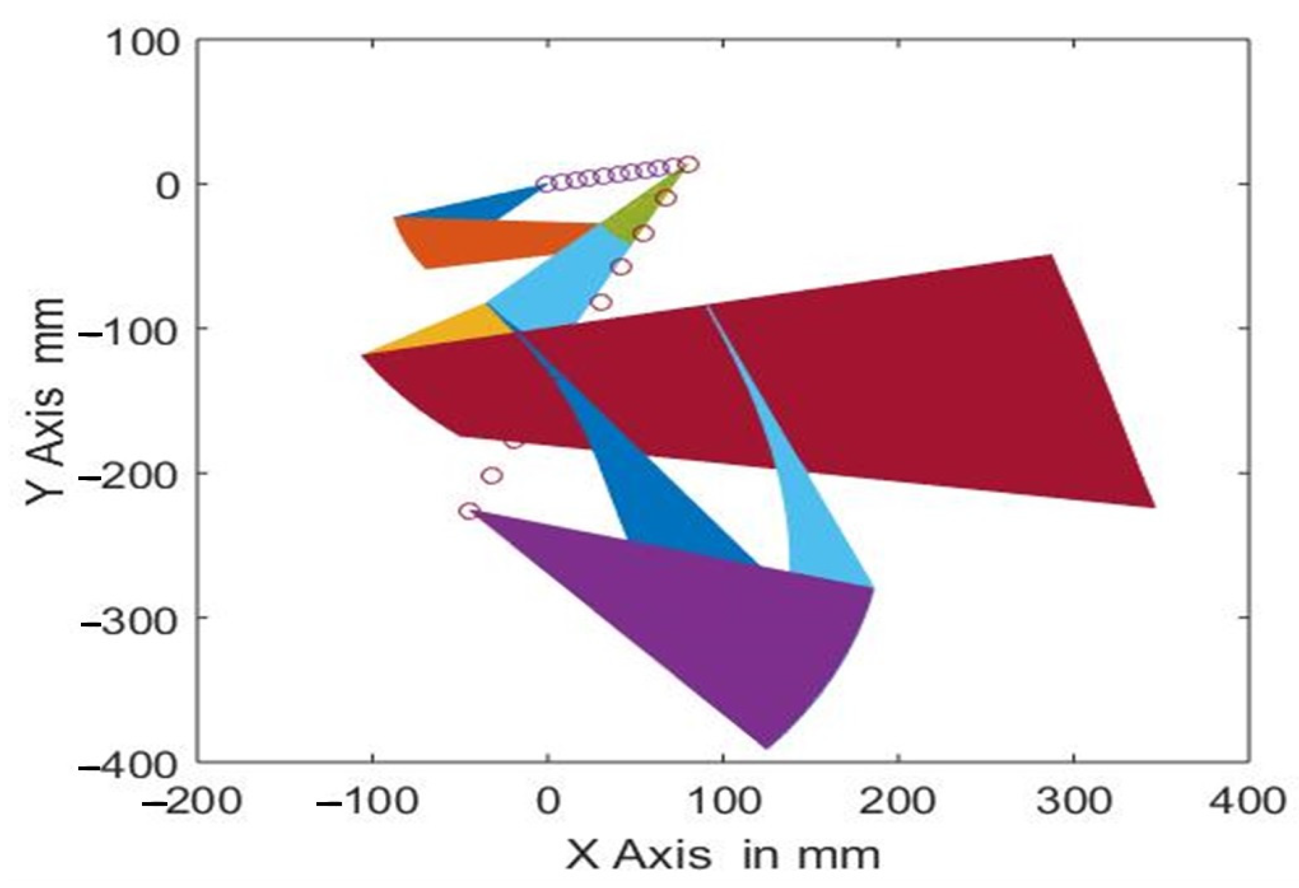
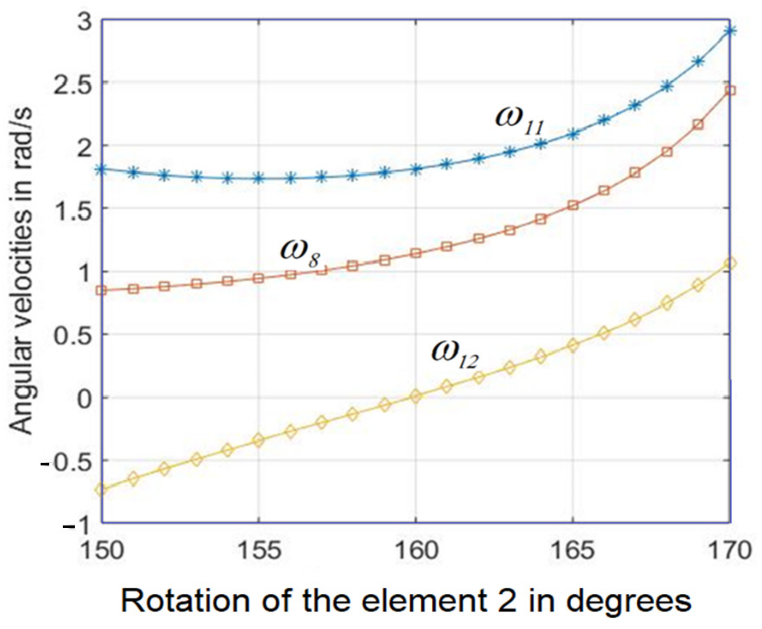
A representation of the different positions of the mechanism in motion is shown in Figure 13 and some computed velocities are presented in Figure 14. To ensure stability of movement, the angular velocity of the flaps must have a variation that is similar or close to the angular velocity of the input element 2. Within the presented application, the angular velocities of several elements of the mechanism were calculated, in case the driving element was operated with a constant angular velocity. The angular velocity ${\omega }_{11}$ which is the speed at which the flap rotates is important in the analysis. For the considered application, we found that this rotation varied quite a bit on the first part of the stroke. On the second part, when the steering angle increased, we also saw an increase in the angular velocity of the flap. It follows that the pilot needs to pay more attention in maneuvering the handle, towards the end of the stroke.

4. Conclusions

The kinematic analysis of a planar mechanism requires, each time, simple but laborious calculations, which use information related to the structure of the mechanism, links, geometries, and various limitations imposed on the technical system by the project. The structural description of the mechanism implies knowledge of the topological structure of the system. Fortunately, graph theory offers a well-developed mathematical tool for the analysis of systems in which topology is an important element in the description of a system.

Regarding the stability and maneuverability problems [6,28,29,30,31] that such a mechanism can pose during flight, the existence of a clear algorithm, depending only on the geometric input data, enables quick calculations and the possibility of making relevant decisions from the design phase. In this sense, the algorithm presented in this paper offers a very powerful, practical, and well-systematized tool for solving this problem. The usefulness of the presented algorithm is demonstrated by performing the kinematic analysis of a light aircraft control mechanism. The results regarding the field of velocities and accelerations of the mechanism elements are obtained easily, quickly, through an easy-to-handle description, using the representations and theorems demonstrated in graph theory.

An advantage of this method is the possibility of organizing the calculus and algorithmizing the process to study such problems. The topology qualitatively and quantitatively describes the structure of the mechanical system, and then it is possible to use the calculation programs provided to automate the results.