Identification of the Domain of the Sturm–Liouville Operator on a Star Graph

Abstract

This article is devoted to the unique recovering of the domain of the Sturm–Liouville operator on a star graph. The domain of the Sturm–Liouville operator is uniquely identified from the set of spectra of a finite number of specially selected canonical problems. In the general case, the domain of the definition of the original operator can be specified by integro-differential linear forms. In the case when the domain of the Sturm–Liouville operator on a star graph corresponds to the boundary value problem, it is sufficient to choose only finite parts of the spectra of canonical problems for a unique identification of the boundary form. Moreover, the above statement is valid only for a symmetric star graph.

1. Introduction

The following result was presented in the well-known work of Borg [1]. The eigenvalues of the problem:

$$-y^{\prime \prime }\left(x\right)+q\left(x\right)y\left(x\right)=\lambda y\left(x\right),0<x<\pi ,$$

(1)

$$y^{\prime }\left(0\right)-hy\left(0\right)=0,y^{\prime }\left(\pi \right)+Hy\left(\pi \right)=0,$$

(2)

are denoted by ${\lambda }_1,{\lambda }_2,\cdots$, where $q\left(x\right)$ is a real-valued function that is continuous on the interval $[0,\pi ]$ and $h,$ H are real numbers. In a similar way, the eigenvalues of Equation (1) with boundary conditions:

$$y^{\prime }\left(0\right)-h_{1}y\left(0\right)=0,y^{\prime }\left(\pi \right)+Hy\left(\pi \right)=0,$$

(3)

are denoted by ${\mu }_1,{\mu }_2,\cdots$, where $h_1\ne h$. Then, the sequences $\left\{{\lambda }_n\right\}$ and $\left\{{\mu }_n\right\}$ uniquely define the function $q\left(x\right)$ and numbers $h,$ $h_1$, and H. Thus, Borg introduced the spectra of two canonical problems $E_1$ and $E_2$. Here:

E₁ is the first canonical problem (1)–(3);

E₂ is the second canonical problem (1)–(2).

The canonical problem $E_2$ coincides with the original problem (1) and (2), which must be recovered from the set of spectra of the canonical problems $E_1$ and $E_2$. The necessary and sufficient conditions are formulated and proven in order for these sequences $\left\{{\lambda }_n\right\}$ and $\left\{{\mu }_n\right\}$ to be two spectra of problems $E_1$ and $E_2$ in [2]. Plaksina [3] studied on the interval $[0,\pi ]$ inverse problems for operators generated by operation $l=(-\frac{d^2}{d{x}^2}+q\left(x\right))$ and general nonseparated self-adjoint boundary conditions, which have the following form:

$$\left\{\begin{array}{c}{y}^{\prime }\left(0\right)+\beta y\left(0\right)+e^{i\alpha }y\left(\pi \right)=0,\hfill \\ y^{\prime }\left(\pi \right)-e^{-i\alpha }y\left(0\right)+\gamma y\left(\pi \right)=0,\hfill \end{array}\right.$$

(4)

where $\alpha ,$ $\beta ,$ $\gamma$ are real numbers. In [3], three canonical problems $E_1,$ $E_2$, and $E_3$ were introduced. By the spectra of these canonical problems, the function $q\left(x\right)$ and numbers $\alpha ,$ $\beta ,$ $\gamma$ can be identified. The canonical problem $E_1$ is given by Equation (1) and separated boundary conditions:

$$y\left(0\right)=0,y^{\prime }\left(\pi \right)+\gamma y\left(\pi \right)=0.$$

(5)

Canonical problem $E_2$ is defined by Equation (1) and nonseparated boundary conditions of the form (4), with parameter $\alpha$ in (4), which should be replaced by ${\alpha }_1$, keeping all other boundary coefficients. Canonical problem $E_3$ coincides with the problem (1)–(4). It turns out that for a unique recovering function $q\left(x\right)$ and numbers $\alpha ,$ $\beta ,$ $\gamma ,$ ${\alpha }_1$, it is not sufficient to give three spectra of canonical problems $E_1,$ $E_2$, and $E_3$. For a unique recovering $q\left(x\right)$, $\alpha ,$ $\beta ,$ $\gamma ,$ ${\alpha }_1$, we need to add to the set of spectra of canonical problems $E_1,$ $E_2$, and $E_3$ a certain set of sign sequences $\left\{{\delta }_n\right\},$ where each of ${\delta }_n$ is either $+1$ or $-1$. We note that in [3], the necessary and sufficient conditions were given for the above four sequences to be three spectra of canonical problems $E_1,$ $E_2$, and $E_3$. Similar inverse spectral problems for differential operators on graphs were studied in [4].

Along with the above-mentioned statements of inverse problems by a set of spectra of canonical problems, it is of interest to study the possibility of uniquely recovering only the boundary conditions of canonical problems. In this case, it is assumed that the coefficient $q\left(x\right)$ of the differential expression is defined on the entire interval $[0,\pi ]$. Such problems are called problems of the identification of boundary conditions [5,6]. Sometimes, this problem is called the problem of identifying the domain of the Sturm–Liouville operator, since the domain of the operator can be specified by different (but equivalent) sets of boundary conditions.

The problems of identifying the boundary conditions of canonical problems usually require a unique recovering of a finite number of boundary coefficients. In the case of Borg, only three real numbers $h,$ $h_1$, and H need to be recovered. In Plaksina’s case, four numbers $\alpha ,$ $\beta ,$ $\gamma$, and ${\alpha }_1$ must be recovered. Hence, it can be understood that to recover a finite number of boundary coefficients, it is not necessary to indicate sets of complete spectra of canonical problems. In [7], it was proven that for a unique recovering of the boundary conditions for higher order differential operators, it is sufficient to indicate only a finite number of eigenvalues from each canonical problem. In this paper, a similar result was proven for the Sturm—Liouville operator on a star graph. Other inverse spectral problems for Dirac operators on a star graph were studied in [8]. In our case, special attention was paid to nonseparated boundary conditions. In brief, we note that Theorem 5 holds only for a symmetric star graph. A star graph with all edges of the same length is called a symmetric star. Consequently, the main result of this article is: uniquely recovering the domain of a second-order differential operator on a star graph is valid only if the graph is symmetric.

Let the ends of the $(m+1)$-th rod be elastically connected to each other at one node. The free ends of m rods are somehow fixed and inaccessible to visual observation. The free visible end of one rod can be hit with a hammer, and the eigenfrequencies of longitudinal vibrations of the coupling structures can be measured. The paper states that there exists a finite set of eigenfrequencies, which uniquely determines the anchoring of the ends of the rods that are inaccessible to visual observation. Such problems are related to the problems of acoustic diagnostics. The mathematical model of the elastic connection of the $(m+1)$-th rod is defined by a star graph on which the Sturm–Liouville operator is defined with some boundary conditions. The paper proved the possibility of uniquely recovering the domain of the Sturm–Liouville operator on a star graph by a set of spectra of special canonical problems. It was proven in the work that a finite number of eigenfrequencies is sufficient for uniquely recovering the fixings of the ends of the rods. Moreover, the total number of eigenfrequencies required for unambiguous restoration of boundary restraints does not exceed $2{(m+1)}^2$. In [9], the problem of recovering the coefficients of differential equations from a finite set of eigenvalues of a boundary value problem with nonseparated boundary conditions was considered.

Identification of the boundary damage for coupling structures consisting of solids remains a challenging topic due to the influence of the solids on each other and experimental conditions. Identification of the boundary damage is difficult if the ends of the coupling structure are not accessible for visual inspection. Therefore, in this work, the eigenfrequencies of longitudinal vibrations of coupling structures were used to identify boundary damage, since the eigenfrequencies of vibrations of connecting structures can be measured by engineering sensors.

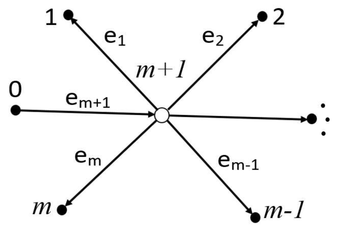
2. Solution of the Cauchy Problem for the Sturm–Liouville Equation on a Star Graph

Let $\Gamma =\{V,E\}$ be a star graph, where V is the set of vertices, numbered from zero to $m+1$ and E is the set of edges $e_1,\cdots ,e_{m+1}$ of the graph $\Gamma =\{V,E\}$ [10]. On each edge $e_j$, the following j-th differential equation:

$$-y_j^{\prime \prime }\left(x_j\right)+p_j\left(x_j\right)y_j\left(x_j\right)=f_j\left(x_j\right),0<x_j<b_j$$

(6)

holds. Further, we assumed that $p_j\left(x\right)$, $j\ge 1$ are real-valued continuous functions on $e_j$. Vertex $(m+1)\in V$ is called the inner vertex of the star graph. At the inner vertex $(m+1)$, Kirchhoff’s laws [11]:

$$\left\{\begin{array}{c}{y}_{m+1}\left(b_{m+1}\right)=y_1\left(0\right)=\cdots =y_m\left(0\right),\hfill \\ y_{m+1}^{\prime }\left(b_{m+1}\right)=y_1^{\prime }\left(0\right)+\cdots +y_m^{\prime }\left(0\right)\hfill \end{array}\right.$$

(7)

hold.

Vertices $0,1,\cdots ,m$ are called boundary vertices of the star graph (Figure 1).

Figure 1. Star graph.

The set of boundary conditions:

$$\begin{array}{cc}\hfill U_k(y_1,\cdots ,y_{m+1})& =\sum _{j=1}^2[{\alpha }_{kj}{y}_1^{(j-1)}\left(b_1\right)+{\alpha }_{k(2+j)}{y}_2^{(j-1)}\left(b_2\right)+\cdots \hfill \\ \hfill & +{\alpha }_{k(2m-2+j)}{y}_m^{(j-1)}\left(b_m\right)+{\alpha }_{k(2m+j)}{y}_{m+1}^{(j-1)}\left(0\right)]=0\hfill \end{array}$$

(8)

holds at the boundary vertices $\{k\in 0,1,\cdots ,m\}$, where ${\alpha }_{ks}$ are complex numbers. Further, it is convenient to introduce the functions $c_j\left(x_j\right),$ $s_j\left(x_j\right),$ $j=1,2,\cdots ,m+1.$ Functions $c_j\left(x_j\right),$ $s_j\left(x_j\right)$ are solutions of the homogeneous differential equations:

$$-y_j^{\prime \prime }\left(x_j\right)+p_j\left(x_j\right)y_j\left(x_j\right)=0,0<x_j<b_j$$

(9)

with initial conditions:

$$\left\{\begin{array}{c}{c}_j\left(0\right)=s_j^{\prime }\left(0\right)=1,c_j^{\prime }\left(0\right)=s_j\left(0\right)=0,j=1,2,\cdots ,m,\hfill \\ c_{m+1}\left(b_{m+1}\right)=s_{m+1}^{\prime }\left(b_{m+1}\right)=1,c_{m+1}^{\prime }\left(b_{m+1}\right)=s_{m+1}\left(b_{m+1}\right)=0\hfill \end{array}\right.$$

for each j. Since the star graph is a tree [12], there exists only one path connecting Vertex 0 to vertex j, where $j=1,\cdots ,m$. We denote this path by $S_j=e_{m+1}\cup e_j$. It is convenient to represent the indicated path $S_j$ as a union of intervals $(0,b_{m+1})$ and $(b_{m+1},b_{m+1}+b_j)$. We introduce the differential equations:

$$-{\phi }^{\prime \prime }\left(x\right)+q_j\left(x\right){\phi }_j\left(x\right)=F_j\left(x\right),x\in (0,b_{m+1})\cup (b_{m+1},b_{m+1}+b_j)$$

(10)

on the unions of intervals $S_j=(0,b_{m+1})\cup \left(b_{m+1},b_{m+1}+b_j\right)$, where:

$$\begin{array}{cc}\hfill & q_j\left(x\right)=p_{m+1}\left(x\right),F_j\left(x\right)=f_{m+1}\left(x\right),\mathrm{if}0<x<b_{m+1},\hfill \\ \hfill & q_j\left(x\right)=p_j\left(x\right),F_j\left(x\right)=f_j\left(x\right),\mathrm{if}{b}_{m+1}<x<b_{m+1}+b_j.\hfill \end{array}$$

We require the following condition:

$${\phi }_j(b_{m+1}-0)={\phi }_j(b_{m+1}+0),A_j{\phi }_j^{\prime }(b_{m+1}-0)={\phi }_j^{\prime }(b_{m+1}+0)$$

(11)

at the point $x=b_{m+1}$, where $\left\{A_j\right\}$ are arbitrary constants subject to a single requirement:

$$A_1+A_2+\cdots +A_m=1.$$

(12)

Let $A_1,A_2,\cdots ,A_m$ be fixed numbers that satisfy the equality (12). We also assume that the functions ${\phi }_j\left(x\right),$ ${\phi }_j^{\prime }\left(x\right)$ are continuous from the left, that is ${\phi }_j(b_{m+1}-0)={\phi }_j\left(b_{m+1}\right),$ ${\phi }_j^{\prime }(b_{m+1}-0)={\phi }_j^{\prime }\left(b_{m+1}\right)$. By ${\Phi }_j\left(x\right)$ and ${\Psi }_j\left(x\right)$, we denote the solutions of Equation (10) with $F_j\left(x\right)\equiv 0$ on the path $S_j$, subject to conditions (11), as well as conditions:

$${\Phi }_j(b_{m+1}-0)={\Psi }_j^{\prime }(b_{m+1}-0)=1,{\Phi }_j^{\prime }(b_{m+1}-0)={\Psi }_j(b_{m+1}-0)=0.$$

(13)

We introduce a particular solution of Equation (10) by the formula:

$${\phi }_j\left(x\right)=\underset{0}{\overset{x}{\int }}\frac{\left|\begin{array}{cc}{\Phi }_j\left(x\right)& {\Psi }_j\left(x\right)\\ {\Phi }_j\left(t\right)& {\Psi }_j\left(t\right)\end{array}\right|}{\left|\begin{array}{cc}{\Phi }_j^{\prime }\left(t\right)& {\Psi }_j^{\prime }\left(t\right)\\ {\Phi }_j\left(t\right)& {\Psi }_j\left(t\right)\end{array}\right|}{F}_j\left(x\right)dt$$

(14)

for any j from the set $\{1,\cdots ,m\}$ and $x\in S_j$. It is clear that the functions ${\phi }_1\left(x\right),{\phi }_2\left(x\right),\cdots ,{\phi }_m\left(x\right)$ defined by Formula (14) satisfy the Kirchhoff conditions (7) at the point $x=b_{m+1}$. Indeed, we can write:

$${\phi }_j\left(x\right)=\underset{0}{\overset{x}{\int }}\left|\begin{array}{cc}{c}_{m+1}\left(x\right)& s_{m+1}\left(x\right)\\ c_{m+1}\left(t\right)& s_{m+1}\left(t\right)\end{array}\right|f_{m+1}\left(t\right)dt,x\in (0,b_{m+1}),$$

$$\begin{array}{cc}\hfill {\phi }_j(x+b_{m+1})& =\underset{0}{\overset{b_{m+1}}{\int }}\left|\begin{array}{cc}{\Phi }_j(x+b_{m+1})& {\Psi }_j(x+b_{m+1})\\ c_{m+1}\left(t\right)& s_{m+1}\left(t\right)\end{array}\right|f_{m+1}\left(t\right)dt\hfill \\ \hfill & +\underset{0}{\overset{x}{\int }}\left|\begin{array}{cc}{c}_j\left(x\right)& s_j\left(x\right)\\ c_j\left(t\right)& s_j\left(t\right)\end{array}\right|f_j\left(t\right)dt,x\in (0,b_j)\hfill \end{array}$$

at $x\in (0,b_{m+1})\cup (b_{m+1},b_{m+1}+b_j)$. We note that the following representation:

$${\Phi }_j(x+b_{m+1})=c_j\left(x\right),{\Psi }_j(x+b_{m+1})=A_j{s}_j\left(x\right)$$

holds for $x\in (0,b_j)$ and the following representation:

$${\Phi }_j\left(x\right)=c_{m+1}\left(x\right),{\Psi }_j\left(x\right)=s_{m+1}\left(x\right)$$

holds for $x\in (0,b_{m+1})$. Thus, we state the following theorem.

Theorem 1.

The solution of the Cauchy problem for the Sturm–Liouville Equations (6) and (7) with Cauchy conditions:

$${\theta }_{m+1}\left(0\right)=0,{\theta }_{m+1}^{\prime }\left(0\right)=0$$

(15)

at the point $x_{m+1}=0$, we denote by $\Theta =({\theta }_1\left(x_1\right),{\theta }_2\left(x_2\right),\cdots ,{\theta }_{m+1}\left(x_{m+1}\right))$, and it has the following representation:

$$\begin{array}{c}\hfill {\theta }_{m+1}\left(x_{m+1}\right)=\underset{0}{\overset{x_{m+1}}{\int }}\left|\begin{array}{cc}{c}_{m+1}\left(x_{m+1}\right)& s_{m+1}\left(x_{m+1}\right)\\ c_{m+1}\left(t\right)& s_{m+1}\left(t\right)\end{array}\right|f_{m+1}\left(t\right)dt,x_{m+1}\in e_{m+1},\end{array}$$

$$\begin{array}{cc}\hfill {\theta }_j\left(x_j\right)& =\underset{0}{\overset{b_{m+1}}{\int }}\left|\begin{array}{cc}{c}_j\left(x_j\right)& A_j{s}_j\left(x_j\right)\\ c_{m+1}\left(t\right)& s_{m+1}\left(t\right)\end{array}\right|f_{m+1}\left(t\right)dt\hfill \\ \hfill & +\underset{0}{\overset{x_j}{\int }}\left|\begin{array}{cc}{c}_j\left(x_j\right)& s_j\left(x_j\right)\\ c_j\left(t\right)& s_j\left(t\right)\end{array}\right|f_j\left(t\right)dt,x_j\in e_j,j=1,2,\cdots ,m,\hfill \end{array}$$

where $A_1,A_2,\cdots ,A_m$ are arbitrary numbers subject to requirement (12).

Remark 1.

Theorem 1 implies that the solution to the Cauchy problem (6), (7), (15) depends on arbitrary $(m-1)$ constants. Constants $A_1,A_2,\cdots ,A_m$ that satisfy the requirement (12) determine at the point $x_{m+1}=b_{m+1}$ the portions of flow along the edges $e_1,e_2,\cdots ,e_m$ with respect to the flow on the edges $e_{m+1}$. The numbers $A_1,A_2,\cdots ,A_m$ we call the connecting constants.

3. Construction of a Biorthogonal System of Solutions for a Set of Boundary Conditions

Let a set of boundary conditions (8) be given by boundary forms $U_0(·),\cdots ,U_m(·).$ The system of solutions $R_j=r_{1j}\left(x_1\right),\cdots ,r_{m+1,j}\left(x_{m+1}\right)$ of the problem (7)–(9) for $j=0,1,\cdots ,m$ is called biorthogonal to the boundary forms $U_0(·),\cdots ,U_m(·)$, if the following requirement:

$$U_k\left(R_j\right)={\delta }_{kj},k,j=0,1,\cdots ,m$$

(16)

holds, where ${\delta }_{kj}$ is the Kronecker delta.

In this section, we find sufficient conditions for the existence of a biorthogonal system of solutions. In other words, what conditions must the set of boundary forms $\{U_k,k=0,1,\cdots ,m\}$ satisfy in order for a biorthogonal system of solutions to the problem (7)–(9) to exist? We introduce the following matrix:

$$T=\left[\begin{array}{cccccc}{U}_0(c_1,c_2,\cdots ,c_{m+1})& U_0^1\left(s_1\right)& U_0^2\left(s_2\right)& \cdots & U_0^m\left(s_m\right)& U_0^{m+1}\left(s_{m+1}\right)\\ U_1(c_1,c_2,\cdots ,c_{m+1})& U_1^1\left(s_1\right)& U_1^2\left(s_2\right)& \cdots & U_1^m\left(s_m\right)& U_1^{m+1}\left(s_{m+1}\right)\\ \cdots \cdots \cdots \cdots \cdots \cdots & \cdots \cdots & \cdots \cdots & \cdots & \cdots \cdots \cdots & \cdots \cdots \cdots \cdots \\ U_m(c_1,c_2,\cdots ,c_{m+1})& U_m^1\left(s_1\right)& U_m^2\left(s_2\right)& \cdots & U_m^m\left(s_m\right)& U_m^{m+1}\left(s_{m+1}\right)\\ 0& 1& 1& \cdots & 1& -1\end{array}\right],$$

where:

$$\begin{array}{cc}\hfill & U_i^k\left(s_k\right)=\sum _{j=1}^2{\alpha }_{i(2k-2+j)}{s}_k^{(j-1)}\left(b_k\right),k\ge 1,i\ge 0,\hfill \\ \hfill & U_i^{m+1}\left(s_{m+1}\right)=\sum _{j=1}^2{\alpha }_{i(2m+j)}{s}_{m+1}^{(j-1)}\left(0\right).\hfill \end{array}$$

(17)

Theorem 2.

Let a set of boundary forms $U_0(·),\cdots ,U_m(·)$ be such that:

$$detT\ne 0.$$

Then, there exists a unique system of solutions to the problem (7)–(9), which is biorthogonal to forms $\{U_0,\cdots ,U_m\}$.

Proof of Theorem 2.

Let us write down the general solution of the homogeneous system of differential Equation (9) subject to the Kirchhoff conditions (7):

$$y_{m+1}\left(x_{m+1}\right)=D{c}_{m+1}\left(x_{m+1}\right)+E{s}_{m+1}\left(x_{m+1}\right),x\in e_{m+1},$$

(18)

$$y_j\left(x_j\right)=D{c}_j\left(x_j\right)+E{A}_j{s}_j\left(x_j\right),x\in e_j,j=1,\cdots ,m.$$

(19)

Here, $D,$ E and $A_1,\cdots ,A_m$ are arbitrary numbers subject to the condition (12). Let us prove that there exist R that satisfy the following equalities:

$$U_0\left(R\right)=1,U_1\left(R\right)=0,\cdots ,U_m\left(R\right)=0.$$

(20)

We seek function $R=(r_1\left(x\right),r_2\left(x\right),\cdots ,r_{m+1}\left(x\right))$ in the forms (18) and (19). By substituting the expressions (18) and (19) into the equalities (20), we obtain a system of algebraic equations with respect to $D,E,A_{1}E,A_{2}E,\cdots ,A_{m}E:$

$$Tz=l_1,$$

(21)

where:

$$z={[D,A_{1}E,A_{2}E,\cdots ,A_{m}E,E]}^T,l_1={[1,0,0,\cdots ,0]}^T.$$

Since $detT\ne 0$, the numbers $E,A_1,A_2,\cdots ,A_m,D$ are uniquely found from the system (21). Therefore, $R_0$ is determined from the conditions (16) for $j=0$ in a unique way. It is also checked in the same way that $R_1,R_2,\cdots ,R_m$ are determined from the conditions (16) for $j\ge 1$ in a unique way. The proof of Theorem 2 is complete. □

4. An Equivalent Set of Boundary Forms That Have an Integral Form

In this section, the set of boundary forms $\{U_0,\cdots ,U_m\}$ from (8) is replaced by an equivalent set of boundary forms $\{W_0,\cdots ,W_m\}$. Let the number $A_m=1-A_1-\cdots -A_{m-1}$ and the numbers $A_1,A_2,\cdots ,A_{m-1}$ be arbitrary numbers. To represent the explicit form of the boundary forms $\{W_0,\cdots ,W_m\},$ we introduce the following functions:

$$\begin{array}{cc}\hfill {\rho }_k^{\left(1\right)}\left(t\right)& =\sum _{i=0}^m{r}_{m+1i}\left(0\right)\left|\begin{array}{cc}{U}_i^k\left(c_k\right)& U_i^k\left(s_k\right)\\ c_k\left(t\right)& s_k\left(t\right)\end{array}\right|,t\in e_k,k\le m,\hfill \\ \hfill {\rho }_{m+1}^{\left(1\right)}\left(t\right)& =\sum _{i=0}^m{r}_{m+1i}\left(0\right)(\left|\begin{array}{cc}{U}_i^{m+1}\left(c_{m+1}\right)& U_i^{m+1}\left(s_{m+1}\right)\\ c_{m+1}\left(t\right)& s_{m+1}\left(t\right)\end{array}\right|\hfill \\ \hfill & +\sum _{i=1}^m\left|\begin{array}{cc}{U}_i^i\left(c_i\right)& A_i{U}_i^i\left(s_i\right)\\ c_{m+1}\left(t\right)& s_{m+1}\left(t\right)\end{array}\right|),t\in e_{m+1},\hfill \\ \hfill {\rho }_k^{\left(2\right)}\left(t\right)& =\sum _{i=0}^m{r}_{m+1i}^{\prime }\left(0\right)\left|\begin{array}{cc}{U}_i^k\left(c_k\right)& U_i^k\left(s_k\right)\\ c_k\left(t\right)& s_k\left(t\right)\end{array}\right|,t\in e_k,k\le m,\hfill \\ \hfill {\rho }_{m+1}^{\left(2\right)}\left(t\right)& =\sum _{i=0}^m{r}_{m+1i}^{\prime }\left(0\right)(\left|\begin{array}{cc}{U}_i^{m+1}\left(c_{m+1}\right)& U_i^{m+1}\left(s_{m+1}\right)\\ c_{m+1}\left(t\right)& s_{m+1}\left(t\right)\end{array}\right|\hfill \\ \hfill & +\sum _{l=1}^m\left|\begin{array}{cc}{U}_i^l\left(c_i\right)& A_i{U}_i^i\left(s_l\right)\\ c_{m+1}\left(t\right)& s_{m+1}\left(t\right)\end{array}\right|),t\in e_{m+1},\hfill \\ \hfill {\rho }_k^{(j+2)}\left(t\right)& =\sum _{i=0}^m(r_{ji}^{\prime }\left(0\right)-A_j{r}_{m+1i}^{\prime }\left(b_{m+1}\right))\left|\begin{array}{cc}{U}_i^k\left(c_k\right)& U_i^k\left(s_k\right)\\ c_k\left(t\right)& s_k\left(t\right),\end{array}\right|t\in e_{m+1},k\le m,\hfill \end{array}$$

$$\begin{array}{cc}\hfill cc{\rho }_{m+1}^{(j+2)}\left(t\right)& =\sum _{i=0}^m(r_{ji}^{\prime }\left(0\right)-A_j{r}_{m+1i}^{\prime }\left(b_{m+1}\right))(\left|\begin{array}{cc}{U}_i^{m+1}\left(c_{m+1}\right)& U_i^{m+1}\left(s_{m+1}\right)\\ c_{m+1}\left(t\right)& s_{m+1}\left(t\right)\end{array}\right|\hfill \\ \hfill & +\sum _{i=1}^m\left|\begin{array}{cc}{U}_i^i\left(c_i\right)& A_i{U}_i^i\left(s_i\right)\\ c_{m+1}\left(t\right)& s_{m+1}\left(t\right)\end{array}\right|),t\in e_{m+1}.\hfill \end{array}$$

(22)

Now, we define new boundary forms by the following formulas:

$$W_0(y_1,y_2,\cdots ,y_{m+1})=y_{m+1}\left(0\right)+\sum _{k=1}^{m+1}\underset{0}{\overset{b_k}{\int }}{\rho }_k^1\left(t\right)(-y_k^{\prime \prime }\left(t\right)+p_k\left(t\right)y_k\left(t\right))dt,$$

$$W_1(y_1,y_2,\cdots ,y_{m+1})=y_{m+1}^{\prime }\left(0\right)+\sum _{k=1}^{m+1}\underset{0}{\overset{b_k}{\int }}{\rho }_k^2\left(t\right)(-y_k^{\prime \prime }\left(t\right)+p_k\left(t\right)y_k\left(t\right))dt,$$

$$\begin{array}{cc}\hfill W_{j+1}(& y_1,y_2,\cdots ,y_{m+1})=y_j^{\prime }\left(0\right)-A_j{y}_{m+1}^{\prime }\left(b_{m+1}\right)\hfill \\ \hfill & +\sum _{k=1}^{m+1}\underset{0}{\overset{b_k}{\int }}{\rho }_k^{j+2}\left(t\right)(-y_k^{\prime \prime }\left(t\right)+p_k\left(t\right)y_k\left(t\right))dt,j=1,\cdots ,m-1.\hfill \end{array}$$

Theorem 3.

Let the problem (6)–(8) have a unique solution $Y=(y_1\left(x\right),y_2\left(x\right),\cdots ,y_{m+1}\left(x\right))$. Then, the set of boundary conditions (8) is equivalent to the following boundary conditions:

$$W_k(y_1,y_2,\cdots ,y_{m+1})=0,k=0,1,\cdots ,m.$$

(23)

The boundary conditions defined by Theorem 1 are called canonical boundary conditions or normalized boundary conditions [7]. Therefore, instead of restoring the boundary conditions (8), we restore the boundary conditions (23).

Remark 2.

We note that the functions ${\rho }_k^{\left(j\right)}\left(t\right)$ for a fixed k from the set $\{1,\cdots ,m+1\}$ are defined on the edge $e_k$ and represent the solutions of the homogeneous Equation (9).

Proof of Theorem 3.

By Theorem 1, we define a solution to the Cauchy problem as follows:

$$\begin{array}{cc}\hfill {\theta }_j\left(x_j\right)& =\underset{0}{\overset{b_{m+1}}{\int }}\left|\begin{array}{cc}{c}_j\left(x_j\right)& A_j{s}_j\left(x_j\right)\\ c_{m+1}\left(t\right)& s_{m+1}\left(t\right)\end{array}\right|f_{m+1}\left(t\right)dt\hfill \\ \hfill & +\underset{0}{\overset{x_j}{\int }}\left|\begin{array}{cc}{c}_j\left(x_j\right)& s_j\left(x_j\right)\\ c_j\left(t\right)& s_j\left(t\right)\end{array}\right|f_j\left(t\right)dt,x_j\in e_j,j=1,2,\cdots ,m,\hfill \\ \hfill {\theta }_{m+1}\left(x_{m+1}\right)& =\underset{0}{\overset{x_{m+1}}{\int }}\left|\begin{array}{cc}{c}_{m+1}\left(x_{m+1}\right)& s_{m+1}\left(x_{m+1}\right)\\ c_{m+1}\left(t\right)& s_{m+1}\left(t\right)\end{array}\right|f_{m+1}\left(t\right)dt,x_{m+1}\in e_{m+1}.\hfill \end{array}$$

(24)

By direct verification, we can check that the following functions:

$${\vartheta }_j\left(x_j\right)={\theta }_j\left(x_j\right)-\sum _{i=0}^m{U}_i\left(\theta \right)r_{ji}\left(x_j\right),j=1,2,\cdots ,m+1$$

(25)

satisfy the boundary condition (8). Let us introduce the notation $V=({\vartheta }_1\left(x_1\right),\cdots ,{\vartheta }_{m+1}\left(x_{m+1}\right)).$ Indeed, the identity $U_i\left(Y\right)=\sum _{k=1}^{m+1}{U}_i^k\left(y_k\right)$ implies that:

$$\sum _{j=1}^{m+1}{U}_0^j\left({\vartheta }_j\right)=\sum _{j=0}^{m+1}{U}_0^j\left({\theta }_j\right)-\sum _{i=0}^m{U}_0\left(\theta \right)\sum _{j=1}^{m+1}{U}_0^j\left(r_{ji}\right).$$

The quantity $U_i^k\left(y_k\right)$ is defined in a similar way as (17). Hence, (16) implies that:

$$U_0\left(V\right)=U_0\left(\theta \right)-\sum _{i=0}^m{U}_i\left(\theta \right)U_0\left(R_i\right)=0,$$

which confirms that the boundary conditions (8) hold. It is not hard to understand that V is a solution to the problem (6)–(8). The uniqueness of the solution to the problem (6)–(8) implies that:

$$Y=V\mathrm{or}{y}_j\left(x_j\right)={\vartheta }_j\left(x_j\right),j=1,2,\cdots ,m+1.$$

(26)

Formulas (25) and (26) imply the following expressions:

$$\begin{array}{c}\hfill {\theta }_j\left(x_j\right)=y_j\left(x_j\right)+\sum _{i=0}^m{U}_i(\Theta )r_{ji}\left(x_j\right),j=1,2,\cdots ,m+1,\end{array}$$

(27)

since $\Theta$ satisfies the following conditions:

$${\theta }_{m+1}\left(0\right)=0,{\theta }_{m+1}^{\prime }\left(0\right)=0,{\theta }_j^{\prime }\left(0\right)-A_j{\theta }_{m+1}^{\prime }\left(b_{m+1}\right)=0,j=1,\cdots ,m-1.$$

(28)

The substitution on the right-hand side of the relations (27) into the conditions (28) gives:

$$\begin{array}{cc}\hfill & y_{m+1}\left(0\right)+\sum _{i=0}^m{U}_i(\Theta )r_{m+1i}\left(0\right)=0,\hfill \\ \hfill & y_{m+1}^{\prime }\left(0\right)+\sum _{i=0}^m{U}_i(\Theta )r_{m+1i}^{\prime }\left(0\right)=0,\hfill \\ \hfill & y_j^{\prime }\left(0\right)-A_j{y}_{m+1}^{\prime }\left(b_{m+1}\right)+\sum _{i=0}^m{U}_m(\Theta )(r_{ji}^{\prime }\left(0\right)\hfill \\ \hfill & -A_j{r}_{m+1i}^{\prime }\left(b_{m+1}\right))=0,j=1,\cdots ,m-1.\hfill \end{array}$$

(29)

Now, we calculate the values $U_0(\Theta ),\cdots ,U_m(\Theta )$ by applying (24). As a result, we have:

$$\begin{array}{cc}\hfill U_i(\Theta )=\sum _{k=1}^{m+1}{U}_i^k\left({\Theta }_k\right)& =\sum _{k=1}^m\underset{0}{\overset{b_{m+1}}{\int }}\left|\begin{array}{cc}{U}_i^k\left(c_k\right)& A_k{U}_i^k\left(s_k\right)\\ c_{m+1}\left(t\right)& s_{m+1}\left(t\right)\end{array}\right|f_{m+1}\left(t\right)dt\hfill \\ \hfill & +\sum _{k=1}^{m+1}\underset{0}{\overset{b_k}{\int }}\left|\begin{array}{cc}{U}_i^k\left(c_k\right)& U_i^k\left(s_k\right)\\ c_k\left(t\right)& s_k\left(t\right)\end{array}\right|f_k\left(t\right)dt\hfill \end{array}$$

(30)

for $i=0,1,\cdots ,m$. We substitute the right-hand side of the relations (30) into the equalities (29), then we have:

$$\begin{array}{c}\hfill \left\{\begin{array}{c}{y}_{m+1}\left(0\right)+\sum _{k=1}^{m+1}\underset{0}{\overset{b_k}{\int }}{\rho }_k^{\left(1\right)}\left(t\right)f_k\left(t\right)dt=0,\hfill \\ y_{m+1}^{\prime }\left(0\right)+\sum _{k=1}^{m+1}\underset{0}{\overset{b_k}{\int }}{\rho }_k^{\left(2\right)}\left(t\right)f_k\left(t\right)dt=0,\hfill \\ y_j^{\prime }\left(0\right)-A_j{y}_{m+1}^{\prime }\left(b_{m+1}\right)\hfill \\ +\sum _{k=1}^{m+1}\underset{0}{\overset{b_k}{\int }}{\rho }_k^{(j+2)}\left(t\right)f_k\left(t\right)dt=0,j=1,\cdots ,m-1.\hfill \end{array}\right.\end{array}$$

(31)

Since $f_k\left(t\right)=-y_k^{\prime \prime }\left(t\right)+p_k\left(t\right)y_k\left(t\right)$ for $k\ge 1$, then the relations (31) imply the proof of Theorem 3. □

5. Selection of Canonical Problems and the Statement of the Inverse Problem

In this section, we present the method for the selection of canonical problems, the spectra of which allow uniquely finding the boundary conditions of the original boundary value problem or the boundary conditions that are equivalent to them. Therefore, it is sufficient to determine the functions:

$$\{{\rho }_k^{\left(j\right)}\left(t\right),k=1,\cdots ,m+1,j=1,\cdots ,m+2\}$$

by the spectra of the canonical problems. In fact, to determine the boundary coefficients we use not the entire spectrum of the auxiliary canonical problem, but only its finite part.

The number of auxiliary canonical problems is equal to the number of edges of the graph-star. Therefore, we build $(m+1)$ canonical problems. As the first canonical problem, we chose the problem (6) and (7) with the following boundary conditions:

$$\begin{array}{cc}\hfill & W_0\left(y\right)=0,y_{m+1}^{\prime }\left(0\right)=0,\hfill \\ \hfill & y_j^{\prime }\left(0\right)-A_j{y}_{m+1}^{\prime }\left(b_{m+1}\right)=0,j=1,\cdots ,m-1.\hfill \end{array}$$

(32)

As a second canonical problem, we chose the problem (6) and (7) with the following boundary conditions:

$$\begin{array}{cc}\hfill & W_0\left(y\right)=0,W_1\left(y\right)=0,\hfill \\ \hfill & y_j^{\prime }\left(0\right)-A_j{y}_{m+1}^{\prime }\left(b_{m+1}\right)=0,j=1,\cdots ,m-1.\hfill \end{array}$$

(33)

In a similar way, we chose the $3\mathrm{rd},4\mathrm{th},\cdots ,(m+1)-\mathrm{th}$ canonical problems. As the $(m+1)-\mathrm{th}$ canonical problem, we chose the problem (6), (7), and (23), which is equivalent to the problem (6)–(8).

We clarify the statement of the problem of recovering the boundary conditions.

The statement of the first problem:

We need to uniquely recover the first boundary vector-function $\{{\rho }_k^{\left(1\right)}\left(t\right),k=1,\cdots ,m+1\}$ by the given differential Equation (6) and by the spectrum of the first canonical problem.

The statement of second inverse problem:

We need to uniquely recover the second boundary vector-function $\{{\rho }_k^{\left(2\right)}\left(t\right),$ $k=1,\cdots ,m+1\}$ by the given differential Equation (6), by boundary vector-function $\{{\rho }_k^{\left(1\right)}\left(t\right),k=1,\cdots ,m+1\}$, and by the spectrum of the second canonical problem.

In a similar way, we state the $3\mathrm{rd},4\mathrm{th},\cdots ,m\mathrm{th}$ inverse problems.

The statement of the $(m+1)\mathrm{th}$ inverse problem:

We need to uniquely recover the $(m+1)\mathrm{th}$ boundary vector-function $\{{\rho }_k^{(m+1)}\left(t\right),$ $k=1,\cdots ,m+1\}$ by the given differential Equation (6), by boundary vector-functions $\left\{{\rho }_k^{\left(1\right)}\left(t\right)\right\},\cdots ,\left\{{\rho }_k^{\left(m\right)}\left(t\right)\right\},k=1,\cdots ,m+1$, and by the spectrum of the $(m+1)\mathrm{th}$ canonical problem. In fact, not the entire spectrum of the canonical problem will be used, but only its end part. This idea is worked out in more detail in the following sections.

6. A Uniqueness Theorem for Recovering Boundary Functions

The transition from the boundary conditions (8) to equivalent canonical boundary forms allows us to prove the uniqueness theorem for the recovery of boundary vector-functions $\{{\rho }_k^{\left(1\right)}\left(t\right),k=1,\cdots ,m+1\},\cdots ,\{{\rho }_k^{(m+1)}\left(t\right),k=1,\cdots ,m+1\}.$ Further, the $s-\mathrm{th}$ canonical problem is called problem $E_s$. We denote by $\stackrel{\sim }{E_s}$ the problem of the type $E_s$ with the same Equation (6), but with different parameters in the boundary conditions (7). Further, we assume that if some symbol denotes an object related to the problem $E_s,$ then the same symbol with a “wave” at the top denotes a similar object of the problem $\stackrel{\sim }{E_s}.$

Theorem 4.

We fix an integer number s in the set $\{1,\cdots ,m+1\}.$ Assume that the spectra of the problems $E_s$ and $\stackrel{\sim }{E_s}$ coincide. If a ${\rho }_k^{\left(1\right)}\left(t\right)={\stackrel{\sim }{\rho }}_k^{\left(1\right)}\left(t\right),\cdots ,{\rho }_k^{(s-1)}\left(t\right)={\stackrel{\sim }{\rho }}_k^{(s-1)}\left(t\right),k=1,\cdots ,m+1$ in $L_2(\Gamma )$ and the systems of the root functions of the problems $E_s$ and $\stackrel{\sim }{E_s}$ are complete in $L_2(\Gamma )$, then ${\rho }_k^{\left(s\right)}\left(t\right)={\stackrel{\sim }{\rho }}_k^{\left(s\right)}\left(t\right)$ on the space $L_2(\Gamma )$.

We introduce [13] in a natural way the metric topology and Lebesgue measure on the graph $\Gamma$. Space $L_2(\Gamma )$ is understood as the $L_2$-space with respect to this measure. In other words, in $L_2(\Gamma )$, we introduce the inner product by the formula:

$$(y,z)=\sum _{j=1}^{m+1}(y_j,z_j)=\sum _{j=1}^{m+1}\underset{0}{\overset{b_j}{\int }}{y}_j\left(x_j\right)\overline{z_j\left(x_j\right)}d{x}_j,y,z\in L_2(\Gamma ).$$

(34)

Then, by (34), the conditions (31) take the following form:

$$\left\{\begin{array}{c}{y}_{m+1}\left(0\right)+<{\rho }^{\left(1\right)},f>=0,\hfill \\ y_{m+1}^{\prime }\left(0\right)+<{\rho }^{\left(2\right)},f>=0,\hfill \\ y_j^{\prime }\left(0\right)-A_j{y}_{m+1}^{\prime }\left(b_{m+1}\right)+<{\rho }^{(j+2)},f>=0,j=1,\cdots ,m-1,\hfill \end{array}\right.$$

where:

$$\begin{array}{cc}\hfill & {\rho }^{\left(1\right)}=({\rho }_1^{\left(1\right)},\cdots ,{\rho }_{m+1}^{\left(j\right)})\in L_2(\Gamma ),\hfill \\ \hfill & f=(f_1,\cdots ,f_{m+1})\in L_2(\Gamma ).\hfill \end{array}$$

We note that $f_t=-y{"}_j\left(t\right)+p_j\left(t\right)y_j\left(t\right),j=1,\cdots ,m+1$. Thus, by our notation, we have:

$$\begin{array}{c}\hfill \left\{\begin{array}{c}{W}_0\left(y\right)=y_{m+1}\left(0\right)+<{\rho }^{\left(1\right)},-y^{\prime \prime }+py>,\hfill \\ W_1\left(y\right)=y_{m+1}^{\prime }\left(0\right)+<{\rho }^{\left(2\right)},-y^{\prime \prime }+py>,\hfill \\ W_{j+1}\left(y\right)=y_j^{\prime }\left(0\right)-A_j{y}_{m+1}^{\prime }\left(b_{m+1}\right)+<{\rho }^{(j+2)},-y"+py>,j=1,\cdots ,m-1,\hfill \end{array}\right.\end{array}$$

(35)

where $py=(p_1{y}_1,p_2{y}_2,\cdots ,p_{m+1}{y}_{m+1})$.

Proof of Theorem 4.

for$\mathbf{s}=\mathbf{1}$. By $u^{\left(1\right)}=(u_1^{\left(1\right)}\left(x_1\right),u_2^{\left(1\right)}\left(x_2\right),\cdots ,u_{m+1}^{\left(1\right)}\left(x_{m+1}\right))$, we denote the solution to the Cauchy problem:

$$\begin{array}{cc}\hfill & -\frac{d^2}{d{x}_j^2}{u}_j^{\left(1\right)}\left(x_j\right)+p_j\left(x_j\right)u_j^{\left(1\right)}\left(x_j\right)=\lambda u_j^{\left(1\right)}\left(x_j\right),x_j\in (0,b_j),j=1,\cdots ,m+1,\hfill \\ \hfill & u_{m+1}^{\left(1\right)}\left(0\right)=1,\frac{d{u}_{m+1}^{\left(1\right)}}{d{x}_{m+1}}\left(0\right)=0,\hfill \\ \hfill & \frac{d{u}_k^{\left(1\right)}\left(x_k\right)}{d{x}_k}{|}_{x_k=0}-A_k\frac{d{u}_{m+1}^{\left(1\right)}\left(x_{m+1}\right)}{d{x}_{m+1}}{|}_{x_{m+1}=b_{m+1}}=0,k=1,\cdots ,m-1.\hfill \end{array}$$

We note that the functions $u_j^{\left(1\right)}(x_j,\lambda )$ are entire functions of the parameter $\lambda$, since, by Theorem 1, the Cauchy problem is uniquely solvable for all complex $\lambda$. Let $\lambda ={\lambda }^{\left(1\right)}$ be the arbitrary eigenvalue of the problem $E_1$. Then,

$$u^{\left(1\right)}\left({\lambda }^{\left(1\right)}\right)=(u_1^{\left(1\right)}(x_1,{\lambda }^{\left(1\right)}),u_2^{\left(1\right)}(x_2,{\lambda }^{\left(1\right)}),\cdots ,u_{m+1}^{\left(1\right)}(x_{m+1},{\lambda }^{\left(1\right)}))$$

is the eigenfunction of the problem $E_1$ corresponding to eigenvalue ${\lambda }^{\left(1\right)}$. The first boundary condition of the problem $E_1$ has the following form:

$$W_0\left(u^1\left({\lambda }^{\left(1\right)}\right)\right)=u_{m+1}^{\left(1\right)}(0,{\lambda }^{\left(1\right)})+{\lambda }^{\left(1\right)}<{\rho }^{\left(1\right)},u^{\left(1\right)}\left({\lambda }^{\left(1\right)}\right)>=0.$$

Hence, it follows that:

$$<{\rho }^{\left(1\right)},u^{\left(1\right)}\left({\lambda }^{\left(1\right)}\right)>=-\frac{1}{{\lambda }^{\left(1\right)}}.$$

Therefore, the eigenvalues of the problem $E_1$ determine the Fourier coefficients of the function ${\rho }^{\left(1\right)}$ in the system of root functions that is conjugate to the problem $E_1$. Since the system of the root functions of the problem $E_1$ is complete in the space $L_2(\Gamma )$, then the system of the root functions of the conjugate problem is also complete in $L_2(\Gamma )$. Thus, if the spectra of the problems $E_s$ and $\stackrel{\sim }{E_s}$ coincide, then the Fourier coefficients of the functions ${\rho }^{\left(1\right)}$ and ${\stackrel{\sim }{\rho }}^{\left(1\right)}$ coincide by the same complete system of the space $L_2(\Gamma )$. Therefore, in the space $L_2(\Gamma )$, functions ${\rho }^{\left(1\right)}$ and ${\stackrel{\sim }{\rho }}^{\left(1\right)}$ coincide. This proof corresponds to the case of the simple eigenvalues of the problems $E_s$ and $\stackrel{\sim }{E_s}$. In the case of multiple eigenvalues, the reasoning requires a slight modification. □

Proof of Theorem 4

for$\mathbf{s}=\mathbf{2}$. By $u^{\left(2\right)}=(u_1^{\left(2\right)}\left(x_1\right),u_2^{\left(2\right)}\left(x_2\right),\cdots ,u_{m+1}^{\left(2\right)}\left(x_{m+1}\right))$, we denote the solution to the Cauchy problem:

$$\begin{array}{cc}\hfill & -\frac{d^2}{d{x}_j^2}{u}_j^{\left(2\right)}\left(x_j\right)+p_j\left(x_j\right)u_j^{\left(2\right)}\left(x_j\right)=\lambda u_j^{\left(2\right)}\left(x_j\right),x_j\in (0,b_j),j=1,\cdots ,m+1,\hfill \\ \hfill & W_0\left(u^{\left(2\right)}\right)=0,\frac{d{u}_{m+1}^{\left(2\right)}}{d{x}_{m+1}}\left(0\right)=0,\hfill \\ \hfill & \frac{d{u}_k^{\left(2\right)}\left(x_k\right)}{d{x}_k}{|}_{x_k=0}-A_k\frac{d{u}_{m+1}^{\left(2\right)}\left(x_{m+1}\right)}{d{x}_{m+1}}{|}_{x_{m+1}=b_{m+1}}=0,k=1,\cdots ,m-1.\hfill \end{array}$$

Let $\lambda ={\lambda }^{\left(2\right)}$ be an arbitrary eigenvalue of the problem $E_2$. Then,

$$u^{\left(2\right)}\left({\lambda }^{\left(2\right)}\right)=(u_1^{\left(2\right)}(x_1,{\lambda }^{\left(2\right)}),u_2^{\left(2\right)}(x_2,{\lambda }^{\left(2\right)}),\cdots ,u_{m+1}^{\left(2\right)}(x_{m+1},{\lambda }^{\left(2\right)}))$$

is the eigenvalue of the problem $E_2$ corresponding to eigenvalue ${\lambda }^{\left(2\right)}$. The second boundary condition of the problem $E_2$ can be represented as follows:

$$\begin{array}{c}\hfill W_1\left(u^{\left(2\right)}\left({\lambda }^{\left(2\right)}\right)\right)=\frac{d}{d{x}_{m+1}}{u}_{m+1}^{\left(2\right)}(x_{m+1},{\lambda }^{\left(2\right)}){|}_{x_{m+1}=0}+{\lambda }^{\left(2\right)}<{\rho }^{\left(2\right)},u^{\left(2\right)}\left({\lambda }^{\left(2\right)}\right)>=0\end{array}$$

Hence, it follows that:

$$<{\rho }^{\left(2\right)},u^{\left(2\right)}\left({\lambda }^{\left(2\right)}\right)>=-\frac{1}{{\lambda }^{\left(2\right)}}.$$

The further reasoning repeats the proof of Theorem 4 for $s=1$. The case, when problems $E_1$ and $E_2$ have common eigenvalues, requires a slight modification in the reasoning. The proofs of Theorem 4 for other s are similar. The proof of Theorem 4 is complete. □

7. Refinement of the Uniqueness Theorem in the Case of Boundary Value Problems

In this section, we refine Theorem 4 for boundary value problems. In Section 4 of this article, we presented Formula (22), which connects the functions ${\rho }_k^{\left(j\right)}\left(x_k\right)$ for $j,k=1,\cdots ,m+1$ with the values of the boundary forms $\{U_i^k\left(c_k\right),U_i^k\left(s_k\right),k=1,\cdots ,m+1,$ $i=1,\cdots ,m+1\}.$ Formula (22) implies that the functions ${\rho }_k^{\left(j\right)}\left(x_k\right)$ for all $j=1,\cdots ,m+1$ are solutions to the homogeneous equations $-y_k^{\prime \prime }\left(x_k\right)+p_k\left(x_k\right)y_k\left(x_k\right)=0,k=1,\cdots ,m+1$. Since the coefficients $p_1\left(x_1\right),\cdots ,p_{m+1}\left(x_{m+1}\right)$ are given, then the solutions $\{c_k\left(x_k\right),s_k\left(x_k\right),$ $k=1,\cdots ,m+1\}$ are also known. We fix j in the set $\{1,\cdots ,m+1\}$.

Let:

$$\begin{array}{c}\hfill {\rho }_k^{\left(j\right)}\left(x_k\right)=h_{1k}^{\left(j\right)}{c}_k\left(x_k\right)+h_{2k}^{\left(j\right)}{s}_k\left(x_k\right),x_k\in (0,b_k),k=1,\cdots ,m+1.\end{array}$$

with unknown constants $h_{1k}^{\left(j\right)},$ $h_{2k}^{\left(j\right)}$. Section 6 of this article provided a connection between the Fourier coefficients of the boundary function ${\rho }^{\left(j\right)}=({\rho }_1^{\left(j\right)}\left(x_1\right),\cdots ,{\rho }_{m+1}^{\left(j\right)}\left(x_{m+1}\right))$ and the given eigenvalues of the problem $E_j$. Recall that:

$$<{\rho }^{\left(j\right)},u^{\left(j\right)}\left({\lambda }^{\left(j\right)}\right)>=-\frac{1}{{\lambda }^{\left(j\right)}},$$

where $u^{\left(j\right)}\left({\lambda }^{\left(j\right)}\right)$ is the eigenfunction of problem $E_j$ corresponding to the eigenvalue ${\lambda }^{\left(j\right)}$.

Consequently, we obtain a system of equations:

$$\begin{array}{c}\hfill \sum _{k=1}^{m+1}\left(h_{1k}^{\left(j\right)}\underset{0}{\overset{b}{\int }}{c}_k\left(x_k\right){\overline{u}}_k^{\left(j\right)}(x_k,{\lambda }^{\left(j\right)})+h_{2k}^{\left(j\right)}\underset{0}{\overset{b}{\int }}{s}_k\left(x_k\right){\overline{u}}_k^{\left(j\right)}(x_k,{\lambda }^{\left(j\right)})\right)=-\frac{1}{{\lambda }^{\left(j\right)}}\end{array}$$

for unknown constants $h_{11}^{\left(j\right)},h_{12}^{\left(j\right)},h_{1m+1}^{\left(j\right)},h_{21}^{\left(j\right)},\cdots ,h_{2m+1}^{\left(j\right)}$. Thus, to uniquely determine the unknown constants $h_{11}^{\left(j\right)},h_{12}^{\left(j\right)},h_{1m+1}^{\left(j\right)},h_{21}^{\left(j\right)},\cdots ,h_{2m+1}^{\left(j\right)}$, it is sufficient to choose eigenvalues $\{{\lambda }_1^{\left(j\right)},{\lambda }_2^{\left(j\right)},\cdots ,{\lambda }_{2m+2}^{\left(j\right)}\}$ of problem $E_j$ so that the determinant $Z=\left(Z_{ij}\right)$ is nonzero, where:

$$\begin{array}{cc}\hfill & Z_{kl+m+1}=\underset{0}{\overset{b_1}{\int }}{s}_l\left(x_l\right){\overline{u}}^{\left(j\right)}(x_l,{\lambda }_k^{\left(j\right)})d{x}_l,\hfill \\ \hfill & Z_{kl}=\underset{0}{\overset{b_l}{\int }}{c}_l\left(x_l\right){\overline{u}}^{\left(j\right)}(x_l,{\lambda }_k^{\left(j\right)})d{x}_l,l=1,\cdots ,m+1,k=1,\cdots ,2m+2.\hfill \end{array}$$

Here, $u^{\left(j\right)}\left({\lambda }_1^{\left(j\right)}\right),\cdots ,u^{\left(j\right)}\left({\lambda }_{2m+2}^{\left(j\right)}\right)$ are eigenfunctions of the problem $E_j$ corresponding to the chosen eigenvalues.

Lemma 1.

Let $b_1=b_2=\cdots =b_{m+1}=b$. Suppose that the coefficients of the differential expressions $p_1\left(x\right),\cdots ,p_{m+1}\left(x\right)$ are chosen so that the system of functions

$\{c_1\left(x\right),s_1\left(x\right),c_2\left(x\right),s_2\left(x\right),\cdots ,c_{m+1}\left(x\right),s_{m+1}\left(x\right)\}$ is linear independent on the interval $[0,b]$. Let problem $E_j$ have infinitely many eigenvalues. Then, there exists a set of eigenvalues $\{{\lambda }_n^{\left(j\right)},n=n_1,\cdots ,n_{2m+2}\}$ of the problem $E_j$ such that the determinant Z is nonzero. Here,

$${\lambda }_1^{\left(j\right)}={\lambda }_{n_1}^{\left(j\right)},\cdots ,{\lambda }_{n_{2m+2}}^{\left(j\right)}={\lambda }_{n_{2m+2}}^{\left(j\right)}$$

are some eigenvalues of the canonical problem $E_j.$

Proof of Lemma 1.

We prove by contradiction. Suppose that for any set of eigenvalues $\{{\lambda }_n^{\left(j\right)},n=n_1,\cdots ,n_{2m+2}\}$ of problem $E_j$, the determinant is equal to zero: Z = 0. We put $n_1=1,\cdots ,n_{2m+1}=2m+1$. Since the problem $E_j$ has infinitely many eigenvalues, assume that ${\lambda }_n^{\left(j\right)},n=n_{2m+2}$ runs through the entire spectrum of the problem $E_j$. Since $Z=0$, then the system of homogeneous linear algebraic equations $Z\overrightarrow{h}=0$ has a nonzero solution, where:

$$\begin{array}{c}\hfill \overrightarrow{h}=[h_{11}^{\left(j\right)},\cdots ,h_{1m+1}^{\left(j\right)}{h}_{21}^{\left(j\right)},\cdots ,h_{2m+1}^{\left(j\right)}]\end{array}$$

has a nonzero solution. We assume that $h_{11}^{\left(j\right)}\ne 0$. Consequently, the Fourier coefficients of the function $c_1\left(x\right)$ are linearly expressed in terms of the Fourier coefficients of the functions $\{s_1\left(x\right),c_2\left(x\right),s_2\left(x\right),\cdots ,c_{m+1}\left(x\right),s_{m+1}\left(x\right)\}$. If all the Fourier coefficients of the function $c_1\left(x\right)$ can be linearly expressed in terms of the Fourier coefficients of the functions $\{s_1\left(x\right),c_2\left(x\right),s_2\left(x\right),\cdots ,c_{m+1}\left(x\right),s_{m+1}\left(x\right)\}$, then the system of functions $\{c_1\left(x\right),s_1\left(x\right),c_2\left(x\right),s_2\left(x\right),\cdots ,c_{m+1}\left(x\right),s_{m+1}\left(x\right)\}$ represents the linear dependent system. We have a contradiction. If $h_{11}^{\left(j\right)}\ne 0$ is not satisfied, then some modification in the reasoning is required. The proof of the lemma is complete. □

Lemma 1 and Theorem 4 imply the following theorem.

Theorem 5.

We fix j in the set $\{1,\cdots ,m+1\}$. Let $b_1=b_2=\cdots =b_{m+1}=b$. Suppose that the coefficients $p_1\left(x\right),\cdots ,p_{m+1}\left(x\right)$ of the differential expressions are chosen so that the system of functions $\{c_1\left(x\right),s_1\left(x\right),c_2\left(x\right),s_2\left(x\right),\cdots ,c_{m+1}\left(x\right),s_{m+1}\left(x\right)\}$ is linear independent on the interval $[0,b]$. Let finite sets of eigenvalues of problems $E_j$ and $\stackrel{\sim }{E_j}$ from Lemma 1 coincide. If ${\rho }^{\left(1\right)}={\stackrel{\sim }{\rho }}^{\left(1\right)},\cdots ,{\rho }^{(j-1)}={\stackrel{\sim }{\rho }}^{(j-1)}$ in $L_2(\Gamma )$, then ${\rho }^{\left(j\right)}={\stackrel{\sim }{\rho }}^{\left(j\right)}$ in $L_2(\Gamma )$.

In the proof of Theorem 4, it was established that the eigenfunctions $E_j$ and $\stackrel{\sim }{E_j}$ coincide if the corresponding eigenvalues coincide. This fact plays an essential role in the proof of Theorem 5. In conclusion, note that some of the constructions presented here can be found in [5,6]. In [14], examples of uniform beams with different boundary anchors having infinitely many identical eigenfrequencies of transverse vibrations were given. In Theorem 5, it was stated that a finite number of eigenfrequencies is sufficient for the unique recovering of boundary anchors. This does not contradict the above results of [14], since Theorem 5 states that the eigenfrequencies must be specially selected for the unique recovering of the boundary anchors of the beam.

8. Conclusions

Boundary value problems for differential equations on compact graphs can be specified by integro-differential conditions. The problem of determining the functions included in the integro-differential conditions is related to inverse problems. The recovery of the functions included in the integro-differential conditions was divided into three steps. In the first step, the integro-differential conditions were reduced to a normalized form. In the second step, we chose the canonical problems, by the spectra of which the integro-differential conditions would be restored. In the final step, a procedure was proposed to restore the functions included in the integro-differential conditions.

The paper proved the possibility of uniquely recovering the domain of the Sturm–Liouville operator on a star graph by the set of spectra of special canonical problems. In a particular case, when the domain of the operator is specified by boundary conditions, then for the unique recovery of the boundary coefficients, it is sufficient to specify only a finite set of its eigenvalues for each canonical problem. The total number of eigenvalues required to uniquely recover the boundary coefficients on a star graph with an $(m+1)$ edge does not exceed $2{(m+1)}^2$. The question of determining the minimum number of eigenvalues for the unique determination of the boundary coefficients seems to be interesting.

In this paper, the first two steps of the recovering of functions included in the integro-differential conditions were described in detail. The third step of the constructive restoration of functions requires its development. Only the recovery scheme was specified here. The modification to the recovery procedure is a question of interest, since interest is growing in the problem connected with identifying the boundary conditions of the differential operators on symmetric graph-like spaces.

The result of the work can be used to detect boundary defects in structures consisting of rods elastically connected in one node. The eigenfrequencies of the longitudinal vibrations of such structures can be measured by technical sensors. Based on the found eigenfrequencies, applying the results of this article, it is possible to identify boundary damage. The results of this article were theoretical, but in the future, they can be brought to constructively realizable algorithms for engineers.

References

- Borg, G. Eine Umkehrung der Storm-Liouvillshen Eigenwertaufgabe. Bestimmung der Differentialgleichung durch die Eigenwerte. Acta Math. 1945, 78, 1–96. [Google Scholar] [CrossRef]
- Levitan, B.M.; Gasymov, M.G. Determination of a differential equation by two of its spectra. Russ. Math. Surv. 1964, 19, 1–63. [Google Scholar] [CrossRef]
- Plaksina, O.A. Inverse problems of spectral analysis for the Storm-Liouville operators with nonseparated boundary conditions. Acta Math. 1988, 59, 1–23. [Google Scholar] [CrossRef]
- Yurko, V. Inverse problems for differential pencils on A-graphs. J. Inverse Ill-Posed Probl. 2017, 25, 819–828. [Google Scholar] [CrossRef]
- Kanguzhin, B.E.; Dairbaeva, G.; Madibaiuly, Z. Uniqueness of the restoration of boundary conditions differential operator on a set of spectra. J. Math. Mech. Comput. Sci. 2019, 104, 44–49. [Google Scholar] [CrossRef]
- Kanguzhin, B.E.; Dairbaeva, G.; Madibaiuly, Z. Identification of boundary conditions of a differential operator. J. Math. Mech. Comput. Sci. 2019, 103, 82–93. [Google Scholar] [CrossRef]
- Kanguzhin, B.E. Recovering of two-point boundary conditions by finite set of eigenvalues of boundary value problems for higher order differential equations. UFA Math. J. 2020, 12, 22–29. [Google Scholar] [CrossRef]
- Liu, D.-Q.; Yang, C.-F. Inverse spectral problems for Dirac operators on a star graph with mixed boundary conditions. Math. Methods Appl. Sci. 2021. [Google Scholar] [CrossRef]
- Sadovnichii, V.; Sultanaev, Y.T.; Akhtyamov, A. The inverse problem of recovering the coefficients of a differential equations on a graph. J. Inverse Ill-Posed Probl. 2020, 28, 727–738. [Google Scholar] [CrossRef]
- Zhapsarbaeva, L.K.; Kanguzhin, B.E.; Seitova, A.A. Asymptotics of the eigenvaluesof the double differentiation operator with Birkhoff-regular boundary conditions on a star graph. Mat. Zhurnal 2018, 18, 107–124. [Google Scholar]
- Ao, S.I.; Gelman, L. Electrical Engineering and Applied Computing; Springer Science+Business Media: New York, NY, USA, 2011. [Google Scholar] [CrossRef]
- Balakrishnan, R.; Ranganathan, K. A Textbook of Graph Theory; Springer Science+Business Media: New York, NY, USA, 2012. [Google Scholar] [CrossRef]
- Sobolev, A.V.; Solomyak, M. Schrodinger operators on homogeneous metric trees: Spectrum in gaps. Rev. Math. Phys. 2002, 14, 421–468. [Google Scholar] [CrossRef] [Green Version]
- Nurakhmetov, D.; Jumabayev, S.; Aniyarov, A.; Kussainov, R. Symmetric Properties of Eigenvalues and Eigenfunctions of Uniform Beams. Symmetry 2020, 12, 2097. [Google Scholar] [CrossRef]
Publisher’s Note: MDPI stays neutral with regard to jurisdictional claims in published maps and institutional affiliations. |
© 2021 by the authors. Licensee MDPI, Basel, Switzerland. This article is an open access article distributed under the terms and conditions of the Creative Commons Attribution (CC BY) license (https://creativecommons.org/licenses/by/4.0/).