Abstract
We summarize our recent work on how to infer on jet formation processes directly from substructure data using generative statistical models. We recount in detail how to cast jet substructure observables’ measurements in terms of Bayesian mixed membership models, in particular Latent Dirichlet Allocation. Using a mixed sample of QCD and boosted jet events and focusing on the primary Lund plane observable basis for event measurements, we show how using educated priors on the latent distributions allows to infer on the underlying physical processes in a semi-supervised way.
1. Introduction
The use of jet substructure techniques in studying large area jets has played an important role in identifying hadronic decays of massive resonances, such as the W [1,2,3] and Higgs [4] bosons, as well as the top [5,6,7,8,9,10,11,12,13,14,15] quark, at the LHC. In the last few years, machine learning (ML) tools have further greatly extended the application of jet substructure in tagging and understanding of hadronic jets [16,17,18,19]. Recently [20,21], we have proposed a new technique to analyse jets and events using tools developed in a branch of ML called generative statistical modeling [22]. Developed primarily to identify emergent themes in collections of documents, these models infer the hidden (or latent) structure of a document corpus using posterior Bayesian inference based on word and theme co-occurrence [23,24,25,26,27,28,29]. Using the example of jet substructure observables based on the clustering history, we have shown how to construct statistical mixed membership models of jet substructure. In particular, using the model of Latent Dirichlet Allocation (LDA) [24], which can be solved efficiently using, e.g., Variational Inference (VI) [30] techniques, we were able to define robust parametric jet and event classifiers. In addition, we have shown that the inference algorithm is able to separate observable patterns corresponding to the massive resonance decays within the signal jets from patterns corresponding to light QCD emissions present within all jets. This is achieved due to the mixed-membership nature of the generative model, where QCD-like patterns found both in the signal and background jets are identified as having been sampled from the same distribution describing QCD-like splittings in the jet substructure. For an extensive comparison of different semi-supervised and unsupervised ML approaches to collider data analysis, including LDA, we refer the reader to two recent community papers [31,32].
The present work serves to provide a pedagogical introduction to statistical mixed membership models and in particular their application to studies of jet substructure first reported in Refs. [20,21]. However, in Section 4 we also discuss the important effects of priors on the latent distributions and how LDA could be used potentially to help estimate and correct for systematic effects in jet substructure measurements and aid the calibration of Monte Carlo simulations. These preliminary results are novel and have not yet been documented elsewhere.
2. Introduction to Mixed Membership Models and LDA for Collider Events
A collider event can be represented by a sequence of observations or measurements taking values in a vector space spanned by a set of physical observables . Each event is, therefore, described by a pattern of points in where the number of points and their position change randomly from event to event. One of the most common examples of this type of event representation are the points patterns describing individual particles in the "natural" hadron collider coordinates or . For most collider events, the corresponding point pattern is not uniformly distributed over . Indeed, a substantial amount of energy from the collision is emitted in the form of hadronic jets leading to clustered points in . The shape and sparsity of the point pattern for each event will of course depend on the observables spanning . Building a completely general probabilistic distribution for events in an arbitrary is, therefore, challenging.
2.1. A Simple Probabilistic Model for Collider Events
In the following, we write down a simple generative probabilistic model for event measurements that is capable of learning the main underlying features in the event. The probabilistic model is based on the three following assumptions: (i) the measurements in each event are exchangeable, (ii) the space of observables is discretized (binned), and (iii) the event measurements are generated from multiple latent probability distributions over .
The first assumption implies that the order in which the measurements are extracted is irrelevant, leading to a joint probability distribution that is permutation invariant , where is any element of the permutation group of N indices. Exchangeability should not be confused with independent and iid (identically distributed). Exchangeability actually implies a weaker notion of statistical independence called ‘conditional independence’. This property can be understood via De Finetti’s representation theorem:
De Finetti’s representation theorem:
A sequence of event measurements is exchangeable if and only if there exists a distribution over some latent space Ω, such that
Notice that if measurements in are assumed exchangeable, then these can be thought as being conditionally independent with respect to a marginalized hidden variable . One can give a Bayesian interpretation to (1), where is a prior and a likelihood.
The next step is to chose a suitable prior and likelihood in (1). We assume that the likelihood is a discrete distribution and that the prior and likelihood are conjugate distributions belonging to the exponential family. We discretize the data by binning and indexing each bin, so that the outcome of any event measurement is in a one-to-one correspondence with the index , M being the total number of bins. From all the discrete distributions in the exponential family, the most natural choice for is the multinomial distribution (a multivariate generalization of the binomial distribution), parametrized by a M-dimensional vector , satisfying
where is the probability that measurement populates the bin. Notice that the space defined by (2) is one of an -dimensional simplex. At this stage, is a free parameter of the model that would need to be fixed. Given that the number of bins is large, it is convenient to introduce a prior distribution for . The only probability distribution over the simplex belonging to the , is the Dirichlet distribution, defined as
The Dirichlet is a family of continuous distributions itself parametrized by a concentration parameter , , where denotes the Gamma function. The concentration parameter controls the shape of the Dirichlet over the simplex. Introducing this Dirichlet prior makes the probabilistic model ’smoother’ since fixing the free parameter of the model now corresponds to choosing the shape of a smooth distribution, whereas before we had to fix independently the parameters of a discrete distribution. The benefit of ‘smoothing’ is a better performance of the model when inferring on the data, especially when measurements are sparse leading to many bins without any measurements.
2.2. Latent Dirichlet Allocation
The last model-building assumption we will make is that the measurements in an event can come from more than one underlying physical source. We assume that are sampled from several latent multinomial distributions , labeled by a finite index and parametrized by . These multinomials, or themes This terminology is imported from topic modelling and natural language processing, where multinomials are distributions defined over a vocabulary representing a specific theme or topic present in a corpus of documents., will each be composed by features coming from a hidden physical process. We take as latent variable the relative proportion of every theme contributing to the event. The likelihood in De Finetti’s event representation is then given by a multinomial mixture model
The discrete distributions are also multinomial distributions parametrized by the latent variable . These represent the probability of selecting a particular theme t for each measurement in the event which is then sampled from . The latent space is, therefore, a -dimensional simplex, denoted by , spanned by the latent mixtures which now satisfy the convexity constraints as in (2). The simplex must not be confused with the simplices defined for each multinomial theme parameters . The most natural choice for the prior in (1) is again a Dirichlet distribution defined over . When putting together the three model-building assumptions discussed above, one arrives to a simple Bayesian generative model for collider events called Latent Dirichlet Allocation (LDA):
LDA was first proposed as a topic model for texts with other topic models have been previously used for collider studies in [33] for quark/gluon jet discrimination [24]. The model has two (multidimensional) model-building hyperparameters controlling the shapes of the Dirichlet distributions: the T-dimensional vector for the theme mixing proportions and a matrix where the M-dimensional row controls the shape of the Dirichlet for the theme multinomials over . The number of themes T must also be fixed before training LDA with data. The simplest possible case is a two-theme LDA model with . In this case, the Dirichlet prior reduces to a beta distribution over the unit interval, and reduces to a binomial distribution over . The generative process for a single collider event reads:
- Draw a random mixing parameter between zero and one from the beta prior.
- Randomly select one of the two themes by drawing from the binomial given .
- Sample one event measurement from the selected theme (i.e., the multinomial over parametrized by ).
- Repeat steps (ii-iii) until all measurements in the event have been generated.
LDA is a special type of Bayesian model known as a mixed-membership model (MMM) because each measurement within an event can come from multiple themes, and each event within an event sample is composed of these themes with different proportions. MMM are generalizations of mixture models and the two are not to be confused with each other. For mixture models, all measurements in an event would be drawn from a single theme (the mixture of themes is then manifest at the event sample level, and not at the event level). MMM are much more flexible probabilistic models that are capable of capturing common features between different underlying physical processes contributing to the event.
2.3. Event Classification with LDA
After fixing the Dirichlet free hyperparameters , and the number of themes , one can use LDA for fully unsupervised event classification tasks. To do this, one calculates using Bayes theorem the posterior distribution . The main point is to learn from unlabelled collider data the theme parameters and use themes to cluster events into two underlying categories, or clusters. One popular learning algorithm used for LDA is variational inference (VI) [24]. During training, the algorithm extracts the themes by identifying recurring measurement patterns, in particular, it identifies co-occurrences between measurements populating different bins throughout the event sample. Once the learning converges and the themes have been extracted, one can compute the likelihood-ratio defined as
The are statistical estimators for the ’s extracted from VI. The classifier is obtained in the usual way by thresholding the likelihood ratio: for some suitable , if then the event belongs to theme , else it belongs to theme . Notice that this classifier depends explicitly on our initial choice for the Dirichlet parameter . In reality, there is a continuous two-dimensional ‘landscape’ of two-theme LDA classifiers. In principle, there is no criteria for choosing one value of over another. A detailed systematic study performed in ref. [21] suggests that a quantity known as perplexity can be used to precisely select the best . The perplexity is a common metric in topic modelling that measures how well the approximated posterior obtained through VI matches the true (intractable) posterior. For given hyperparameters , the perplexity is thus a criteria for the convergence of the algorithm. It can also be useful to distinguish between different sets of hyperparameters because it is related to the lower bound of the probability of measuring the data given the hyperparameters, or evidence of the model. However, as we do not have an upper bound on the evidence this lower bound is not enough to provide a bound on the Bayes factor between the competing models. What we showed in ref. [21] is that the perplexity is still enough to select a set of hyperparameters by virtue of being correlated with the performance of the likelihood-ratio classifier.
3. LDA for Jet Substructure
The experimental data we have so far considered in our work consists solely of jets, although the LDA technique could also be applied to final states with different types of objects such as leptons, missing transverse energy or directly to low-level observables such as calorimeter tracks. To make use of it, we must be careful to choose a representation of the experimental data such that it fits into the probabilistic framework outlined in the previous section. One such representation that meets these requirements is in terms of the Lund plane observables [34,35].
To obtain the Lund plane representation for a single jet we start by re-clustering it using the C/A algorithm. This algorithm uses the distance in the plane as a metric to perform a pairwise iterative clustering of the constituents, and being the pseudo-rapidity and the azimuthal angle defined in the laboratory frame. This re-clustering continues until all constituents (and subjets) are clustered into one jet with a maximum radius R. The Lund plane representation follows from undoing this clustering piece by piece. At each step, we split a subjet into two further subjets, , where are referred to as the daughter subjets and as the parent subjet. From them, we calculate the observables
We then assign each splitting to a primary, secondary, etc Lund plane using the simple algorithm:
- uncluster
- assign to the daughter with the larger (smaller)
- perform the next step in the unclustering, e.g.,
- assign to the daughter with the larger (smaller)
- add the l from the parent to the l’s assigned to the daughters and
- repeat steps 3–5 until the jet is completely unclustered.
At the end, each splitting comes with a set of observables and an l-value. We identify as the primary Lund plane, as the secondary Lund plane, and so on. This way the primary Lund plane contains all splittings from the hardest -core of the jet, while the secondary Lund plane contains splittings once removed from this hardest -core, and so on. In the following, we focus on just the primary Lund splittings, and on the observables.
To establish a connection with the previous section, the splittings in the jet are denoted by with i labelling the splitting. The latent parameters denoting the theme refer in this case to a mixture of different physical processes occurring while the jet forms in the detector. For example, a QCD jet would consist of splittings which are entirely described by QCD splitting functions, whereas top jets would consist partially of these QCD splttings and partially of splittings related to the hard decay of the top quark to a W boson and a bottom quark. To see that this Lund plane representation fits into the probabilistic structure of LDA we only need to note that each splitting in the jet is independent of the other splittings, up to the underlying physical processes at play during its formation, i.e., the latent themes.
Features in the jet substructure, such as the decay of a top quark or some other relatively heavy particle, then correspond to features in the primary Lund plane which can be uncovered through statistical inference using the LDA model. In the next section, we will see an explicit implementation of this idea with data.
4. Example: Mixed Samples of QCD and Top Jets
We demonstrate our technique using boosted top quark pair-production. Since our model is built to learn from jet substructure, we consider only the hadronic final states of the W bosons . Consequently, the main background process is QCD di-jet production. In recent years, this process has become a standard benchmark for supervised machine learning applications to particle physics [36]. Although there is no need for an unsupervised top tagging algorithm, it is a nice example that demonstrates the power of LDA by applying it to a well measured and understood physical process.
All event samples are generated using MadGraph5_aMC@NLO [37] interfaced with Pythia 8 [38] for showering and hadronization, and FastJet 3.4.1 [39] for jet clustering. The events are generated at a collision energy of 13 TeV and the jets are clustered using the CA algorithm [40,41] with . No jet grooming is performed. Jets with GeV are discarded. The detector effects are not simulated, although we have verified that the effects of subcluster energy smearing consistent with the Delphes 3 [42] simulation of the ATLAS detector have no significant effect on our results.
In addition to the primary Lund basis observables, we also implement jet labels to represent the data. Although in the considered benchmark example the ordering of the jets is not crucial for performance, since both jets in the event are top jets and have the same decay structure, one can easily imagine other signals where this might not be the case. Even more, being able to differentiate between these different structures is not just important for classification, but is also important for a physical interpretation of the themes learned through the VI algorithm. Therefore, in the case where the signal events contain two different jets, we would like to be able to associate the labels with splittings from one jet or the other, consistently across the whole sample. This will not happen if we label the jets by their , thus, instead, we order the jets according to their jet mass , such that . We plot the pure signal ( jets) and background (QCD di-jets) samples in the plane, in Figure 1. In said Figure, we see that the splittings corresponding to the hard decays of the top quark and the W boson are indicated by the two overlapping clusters at and . This choice of observable basis leads to a large overlap between the background and signal distributions, as seen by the stream of splittings at low . However, there are still clearly discernible differences between the features that allow us to distinguish events from the QCD background.
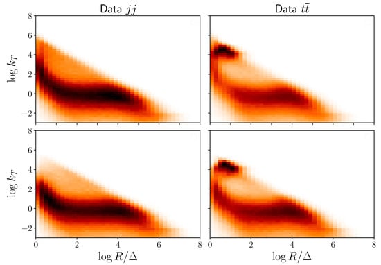
Figure 1.
Distributions of QCD (left) and (right) di-jet events in the (, ) plane. See text for details.
With the simulated events at hand, we define the LDA model and perform Bayesian inference on the themes and theme weights using Variational Inference. We do this by using the Gensim package [43]. As detailed in Ref. [21], LDA possesses several hyperparameters, some related to the VI procedure such as the learning rate, the offset and the chunksize and some related to the model itself such as and . In Ref. [21] we explored the influence of the former on the convergence and performance of the LDA theme learning. In particular, we have shown how the perplexity can be used to determine the theme fraction hyperparameters , which are close to optimal from a tagging perspective. To do this, we kept the theme hyperparameters fixed.
In this work, we are interested in using LDA to recover the underlying distributions shown in Figure 1 from a corpus of events where the signal is not rare. We consider 45 × total events, where 30 × originate from QCD di-jet events and 15 × from production. This case is similar to the second row of Figures 13 and 14 in Ref. [21] albeit with less total events.
As we are not interested in classification itself but only on recovering the themes, we do not perform a hyperparameter scan on to find the best possible choice from a tagging perspective. Instead, we consider a fixed set which provides a reasonable reconstruction performance, something to be expected given the hyperparameter scan for fixed detailed in ref. [21]. Although performing the scan could provide us with quantitatively better results, the qualitative behavior we are interested in would be very similar. In the present work, we instead focus on the priors for the themes themselves (given by hyperparameters ). Contrary to a fully unsupervised approach, we thus perform a semi-supervised analysis where we prime the LDA with information about the approximate shapes of the themes to recover. We consider the following priors for the themes:
where , are two probability distributions over the vocabulary of size V and , are two normalization factors. The role of and can be understood by looking at the mean and variance of a given theme probability
From these equations, one sees that represent the expected distributions while controls the confidence we have in that expectation. Using this parameterization, we consider two cases: (a) uniform prior and (b) smeared/distorted representation of the observable distributions. These two cases are shown in Figure 2. The former case (a) is the default one we considered previously in Refs. [20,21] and is suited for unsupervised analyses of the data. The latter (b) encodes a more realistic case, where we have a fairly reasonable idea of what we expect but we do not trust the Monte Carlo simulations and thus want to perform a semi-supervised analysis where the algorithm can improve upon our imperfect knowledge of the data. In our example, where the “true” distributions are obtained from Monte Carlo simulations, we construct the imperfect estimate (b) by smearing the energies of each final state particle for each event of our simulated dataset Other options would be to use different Monte Carlo tunes to generate different datasets, or to use parton shower level distributions when inferring the themes from simulated detector level reconstructed events. We consider our choice of a smeared Monte Carlo as representative of a crude or inexact estimation of the data.
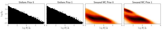
Figure 2.
Left (Right) columns: Probability distributions of the uniform (smeared Monte Carlo) prior. We only show the leading jet themes, with the subleading jets exhibiting a similar behavior.
We perform the inference in LDA for the two sets of theme priors using different degrees of confidence. We consider the special case to reduce the number of hyperparameters to scan. We consider different values of between and . The range of we consider takes into account that the interplay between prior and likelihood is roughly dictated by the relation between and the frequencies of the words. As we consider 45,000 documents with 15,000 belonging to and assuming each jet has no more than two or three hard splittings, the appropriate scale where prior and likelihood are similar is of order . Given that, in practice, one does not know the appropriate scale, we scan over a broader range of and study the learned themes for each choice. We show the obtained themes for the two sets of priors with a good choice in Figure 3.
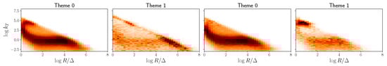
Figure 3.
Left (right) columns: The obtained theme distributions using uniform (smeared Monte Carlo) priors and . We only show the leading jet themes, with the subleading jets exhibiting a similar behavior.
For lower , the inference procedure is too likelihood-dominated and different priors yield equivalent results. In this case, the performance of the algorithm is sub-optimal with the two themes picking up mostly QCD features. For higher , the inference procedure is too prior-dominated and the obtained themes are very similar to the initial . For intermediate values of where the prior and likelihood influences are comparable, different priors yield different results and so we can guide the performance of the algorithm. This is the case for shown in Figure 3. In this case, we see that the use of smeared Monte Carlo simulations to perform semi-supervised analysis yields better results compared to when using flat priors. The latter yields a data-like theme (0) where QCD and hard top-decay features are blended together, and a noise-like theme (1) where some hard features populate the highest probability bins, but do not correspond to physical top-decay distributions. On the other hand, LDA with smeared Monte Carlo priors is able to identify correctly the hard top-decay features and assign the appropriate cluster the highest probability in the second theme (1). Importantly, these hard splittings are not the same as the ones present in the prior, although they are close in the primary Lund plane. It is also able to correct the mismodelled (prior) QCD features of this top-like theme. However, because LDA captures archetypes, it assigns low probabilities to these QCD-like features, which conversely dominate the background-theme (0). Similarly, we observe that this QCD-like theme (0) moves away from its prior and now closely resembles the true QCD jet substructure distribution.
5. Conclusions
In this work, we have reviewed a general unsupervised machine learning (ML) framework capable of learning rare patterns in event data collected at high-energy colliders: the Bayesian probabilistic modeling technique called Latent Dirichlet Allocation (LDA). By representing individual collider events as sequences of binned exchangeable measurements, we have constructed a simplified picture in which the events are generated by sampling these measurements from some underlying joint probability distribution. The assumption of exchangeability of measurements guarantees, through de Finnetti’s theorem, that the sequence of measurements in an event are conditionally dependent on a latent variable sampled from a (marginalised over) prior distribution over a latent space. Through some basic assumptions on this latent space, one arrives at the Bayesian generative model of LDA. LDA is a mixed-membership model, meaning that the measurements in individual events are assumed to have been sampled from multiple (two, in our case) different multinomial distributions – themes. These themes encode information on the underlying structure, i.e., hidden patterns, in the event data represented in terms of binned measurements. The mixing proportions of themes are sampled from a prior taking the form of a Dirichlet distribution, a parametric family of distributions over the simplex. Mixed membership models have the advantage of describing different events which share features arising from the same underlying physical source.
To demonstrate the power of this technique, we considered the analysis of di-jet events at the LHC focusing on the benchmark example of boosted SM production. We described how to pre-process the event data to express each event as a sequence of exchangeable measurements, and how the generative model for di-jet events is to be interpreted using LDA. Our choice of jet substructure observables in the Lund plane basis [34] for the analysis is based upon high level observable combinations that have previously been shown to be good for identifying massive resonance decay chains within large radius jets with supervised methods.
We have demonstrated how the extracted themes hold valuable information about the signal and background processes. In particular, the features in the probability distributions over the kinematical observables of the two uncovered themes match to a high degree the expected features of the underlying hard processes—hadronic decays of top-quarks and the QCD background, respectively, allowing for an intuitive and physical understanding of what the algorithm has learned.
From the results, it is clear that the inference algorithm was able to separate measurement patterns corresponding to the massive resonance decays within the signal jets from patterns corresponding to light QCD emissions present within all jets. This is achieved due to the mixed-membership nature of the generative model, where QCD-like patterns found both in the signal and background jets were identified as having been sampled from the same theme describing QCD-like splittings in the jet substructure.
Going beyond previously published results, we have explored the possibility of introducing non-trivial theme priors into the algorithm. Well-motivated (e.g., based on Monte Carlo simulations) priors allow to perform a semi-supervised analysis where the algorithm starts with an imperfect Monte Carlo based estimates of the observable distributions, and improves them after training on real data collected by the experiments. This is achieved by a balance between the likelihood and the prior weights which we encode in the hyperparameters. We have shown how this works in practice for the production example where the advantage of considering priors to recover realistic latent distributions over starting from uniform priors is clear. Introducing theme priors opens new possibilities as one could differentiate between background and signal theme priors or implement general types of priors which are sensitive to many different signals. One compelling example is 4-top production where current Monte Carlo simulations of signal and background distributions do not describe the observed data well. Introducing Monte Carlo-based SM background and signal theme priors, it could thus be possible to cover many potential New Physics possibilities where conventional analyses may be sub-optimal [44]. In this sense, priors can be regarded as another set of hyperparameters which allow LDA enough flexibility to deal with the complexity of LHC data. A more systematic study of LDA priors is in progress and the results will be published elsewhere.
Author Contributions
Conceptualization, B.M.D., D.A.F., J.F.K. and M.S.; methodology, B.M.D., D.A.F., J.F.K. and M.S.; software, B.M.D., D.A.F., J.F.K. and M.S.; validation, B.M.D., D.A.F., J.F.K. and M.S., formal analysis, B.M.D., D.A.F., J.F.K. and M.S.; investigation B.M.D., D.A.F., J.F.K. and M.S.; resources, B.M.D., D.A.F., J.F.K. and M.S.; data curation, B.M.D., D.A.F., J.F.K. and M.S.; writing—original draft preparation, B.M.D., D.A.F., J.F.K. and M.S.; writing—review and editing, B.M.D., D.A.F., J.F.K. and M.S.; visualization, B.M.D., D.A.F., J.F.K. and M.S.; supervision, B.M.D., D.A.F., J.F.K. and M.S.; project administration, B.M.D., D.A.F., J.F.K. and M.S.; funding acquisition, B.M.D., D.A.F., J.F.K. and M.S. All authors have read and agreed to the published version of the manuscript.
Funding
J.F.K. acknowledges the financial support from the Slovenian Research Agency (research core funding No. P1-0035). This article is based upon work from COST Action CA16201 PARTICLEFACE supported by COST (European Cooperation in Science and Technology). D.A.F. has received funding from the European Research Council (ERC) under the European Union’s Horizon 2020 research and innovation programme under grant agreement 833280 (FLAY), and by the Swiss National Science Foundation (SNF) under contract 200021-175940.
Institutional Review Board Statement
Not applicable.
Informed Consent Statement
Not applicable.
Data Availability Statement
Not applicable.
Conflicts of Interest
The authors declare no conflict of interest.
References
- Butterworth, J.M.; Cox, B.E.; Forshaw, J.R. WW scattering at the CERN LHC. Phys. Rev. 2002, D65, 096014. [Google Scholar] [CrossRef] [Green Version]
- Butterworth, J.M.; Ellis, J.R.; Raklev, A.R. Reconstructing sparticle mass spectra using hadronic decays. JHEP 2007, 05, 033. [Google Scholar] [CrossRef]
- Cui, Y.; Han, Z.; Schwartz, M.D. W-jet Tagging: Optimizing the Identification of Boosted Hadronically-Decaying W Bosons. Phys. Rev. 2011, D83, 074023. [Google Scholar] [CrossRef] [Green Version]
- Butterworth, J.M.; Davison, A.R.; Rubin, M.; Salam, G.P. Jet substructure as a new Higgs search channel at the LHC. Phys. Rev. Lett. 2008, 100, 242001. [Google Scholar] [CrossRef] [Green Version]
- Skiba, W.; Tucker-Smith, D. Using jet mass to discover vector quarks at the LHC. Phys. Rev. 2007, D75, 115010. [Google Scholar] [CrossRef] [Green Version]
- Holdom, B. t-prime at the LHC: The Physics of discovery. JHEP 2007, 03, 063. [Google Scholar] [CrossRef]
- Gerbush, M.; Khoo, T.J.; Phalen, D.J.; Pierce, A.; Tucker-Smith, D. Color-octet scalars at the CERN LHC. Phys. Rev. 2008, D77, 095003. [Google Scholar] [CrossRef] [Green Version]
- Kaplan, D.E.; Rehermann, K.; Schwartz, M.D.; Tweedie, B. Top Tagging: A Method for Identifying Boosted Hadronically Decaying Top Quarks. Phys. Rev. Lett. 2008, 101, 142001. [Google Scholar] [CrossRef]
- Almeida, L.G.; Lee, S.J.; Perez, G.; Sung, I.; Virzi, J. Top Jets at the LHC. Phys. Rev. 2009, D79, 074012. [Google Scholar] [CrossRef]
- Almeida, L.G.; Lee, S.J.; Perez, G.; Sterman, G.F.; Sung, I.; Virzi, J. Substructure of high-pT Jets at the LHC. Phys. Rev. 2009, D79, 074017. [Google Scholar] [CrossRef] [Green Version]
- Almeida, L.G.; Lee, S.J.; Perez, G.; Sterman, G.; Sung, I. Template Overlap Method for Massive Jets. Phys. Rev. 2010, D82, 054034. [Google Scholar] [CrossRef] [Green Version]
- Backovic, M.; Juknevich, J. TemplateTagger v1.0.0: A Template Matching Tool for Jet Substructure. Comput. Phys. Commun. 2014, 185, 1322–1338. [Google Scholar] [CrossRef] [Green Version]
- Plehn, T.; Salam, G.P.; Spannowsky, M. Fat Jets for a Light Higgs. Phys. Rev. Lett. 2010, 104, 111801. [Google Scholar] [CrossRef] [Green Version]
- Plehn, T.; Spannowsky, M.; Takeuchi, M.; Zerwas, D. Stop Reconstruction with Tagged Tops. JHEP 2010, 10, 078. [Google Scholar] [CrossRef] [Green Version]
- Soper, D.E.; Spannowsky, M. Finding top quarks with shower deconstruction. Phys. Rev. 2013, D87, 054012. [Google Scholar] [CrossRef] [Green Version]
- Nachman, B. A guide for deploying Deep Learning in LHC searches: How to achieve optimality and account for uncertainty. SciPost Phys. 2020, 8, 090. [Google Scholar] [CrossRef]
- Larkoski, A.J.; Moult, I.; Nachman, B. Jet Substructure at the Large Hadron Collider: A Review of Recent Advances in Theory and Machine Learning. Phys. Rept. 2020, 841, 1–63. [Google Scholar] [CrossRef] [Green Version]
- Guest, D.; Cranmer, K.; Whiteson, D. Deep Learning and its Application to LHC Physics. Ann. Rev. Nucl. Part. Sci. 2018, 68, 161–181. [Google Scholar] [CrossRef] [Green Version]
- Bollweg, S.; Haußmann, M.; Kasieczka, G.; Luchmann, M.; Plehn, T.; Thompson, J. Deep-Learning Jets with Uncertainties and More. SciPost Phys. 2020, 8, 006. [Google Scholar] [CrossRef] [Green Version]
- Dillon, B.M.; Faroughy, D.A.; Kamenik, J.F. Uncovering latent jet substructure. Phys. Rev. D 2019, 100, 056002. [Google Scholar] [CrossRef] [Green Version]
- Dillon, B.; Faroughy, D.; Kamenik, J.; Szewc, M. Learning the latent structure of collider events. JHEP 2020, 10, 206. [Google Scholar] [CrossRef]
- Bishop, C.M. Pattern Recognition and Machine Learning; Information science and statistics; Springer: New York, NY, USA, 2006; Softcover published in 2016. [Google Scholar]
- Blei, D.M. Probabilistic Topic Models. Commun. ACM 2012, 55, 77–84. [Google Scholar] [CrossRef] [Green Version]
- Blei, D.M.; Ng, A.Y.; Jordan, M.I.; Lafferty, J. Latent dirichlet allocation. J. Mach. Learn. Res. 2003, 3, 2003. [Google Scholar]
- Griffiths, T.L.; Steyvers, M. Finding scientific topics. Proc. Natl. Acad. Sci. USA 2004, 101, 5228–5235. [Google Scholar] [CrossRef] [Green Version]
- Pritchard, J.K.; Stephens, M.; Donnelly, P. Inference of Population Structure Using Multilocus Genotype Data. Genetics 2000, 155, 945–959. [Google Scholar] [CrossRef]
- Hofmann, T. Probabilistic Latent Semantic Analysis. arXiv 1999, arXiv:1301.6705. [Google Scholar]
- Deerwester, S.; Dumais, S.T.; Furnas, G.W.; Landauer, T.K.; Harshman, R. Indexing by latent semantic analysis. J. Am. Soc. Inf. Sci. 1990, 41, 391–407. [Google Scholar] [CrossRef]
- Nigam, K.; Mccallum, A.K.; Thrun, S.; Mitchell, T. Text Classification from Labeled and Unlabeled Documents using EM. Mach. Learn. 1999, 39, 103–134. [Google Scholar] [CrossRef] [Green Version]
- Blei, D.M.; Kucukelbir, A.; McAuliffe, J.D. Variational Inference: A Review for Statisticians. J. Am. Stat. Assoc. 2017, 112, 859–877. [Google Scholar] [CrossRef] [Green Version]
- Kasieczka, G.; Nachman, B.; Shih, D.; Amram, O.; Andreassen, A.; Benkendorfer, K.; Bortolato, B.; Brooijmans, G.; Canelli, F.; Collins, J.H.; et al. The LHC Olympics 2020: A Community Challenge for Anomaly Detection in High Energy Physics. arXiv 2021, arXiv:2101.08320. [Google Scholar]
- Aarrestad, T.; van Beekveld, M.; Bona, M.; Boveia, A.; Caron, S.; Davies, J.; De Simone, A.; Doglioni, C.; Duarte, J.M.; Farbin, A.; et al. The Dark Machines Anomaly Score Challenge: Benchmark Data and Model Independent Event Classification for the Large Hadron Collider. arXiv 2021, arXiv:2105.14027. [Google Scholar]
- Metodiev, E.M.; Thaler, J. Jet Topics: Disentangling Quarks and Gluons at Colliders. Phys. Rev. Lett. 2018, 120, 241602. [Google Scholar] [CrossRef] [Green Version]
- Dreyer, F.A.; Salam, G.P.; Soyez, G. The Lund Jet Plane. JHEP 2018, 12, 064. [Google Scholar] [CrossRef] [Green Version]
- Carrazza, S.; Dreyer, F.A. Lund jet images from generative and cycle-consistent adversarial networks. Eur. Phys. J. C 2019, 79, 979. [Google Scholar] [CrossRef] [Green Version]
- Butter, A.; Plehn, T.; Butter, A.; Cranmer, K.; Debnath, D.; Dillon, B.M.; Fairbairn, M.; Faroughy, D.A.; Fedorko, W.; Gay, C.; et al. The Machine Learning Landscape of Top Taggers. SciPost Phys. 2019, 7, 014. [Google Scholar] [CrossRef] [Green Version]
- Alwall, J.; Frederix, R.; Frixione, S.; Hirschi, V.; Maltoni, F.; Mattelaer, O.; Shao, H.S.; Stelzer, T.; Torrielli, P.; Zaro, M. The automated computation of tree-level and next-to-leading order differential cross sections, and their matching to parton shower simulations. JHEP 2014, 07, 079. [Google Scholar] [CrossRef] [Green Version]
- Sjöstrand, T.; Ask, S.; Christiansen, J.R.; Corke, R.; Desai, N.; Ilten, P.; Mrenna, S.; Prestel, S.; Rasmussen, C.O.; Skands, P.Z. An Introduction to PYTHIA 8.2. Comput. Phys. Commun. 2015, 191, 159. [Google Scholar] [CrossRef] [Green Version]
- Cacciari, M.; Salam, G.P.; Soyez, G. FastJet User Manual. Eur. Phys. J. 2012, C72, 1896. [Google Scholar] [CrossRef] [Green Version]
- Dokshitzer, Y.L.; Leder, G.D.; Moretti, S.; Webber, B.R. Better jet clustering algorithms. JHEP 1997, 08, 001. [Google Scholar] [CrossRef]
- Wobisch, M.; Wengler, T. Hadronization Corrections to Jet Cross-Sections in Deep Inelastic Scattering. Monte Carlo Generators for HERA Physics. arXiv 1998, arXiv:hep-ph/9907280. [Google Scholar]
- de Favereau, J.; Delaere, C.; Demin, P.; Giammanco, A.; Lemaître, V.; Mertens, A.; Selvaggi, M. DELPHES 3, A modular framework for fast simulation of a generic collider experiment. JHEP 2014, 02, 057. [Google Scholar] [CrossRef] [Green Version]
- Řehůřek, R.; Sojka, P. Software Framework for Topic Modelling with Large Corpora. In Proceedings of the LREC 2010 Workshop on New Challenges for NLP Frameworks, Valletta, Malta, 22 May 2010; pp. 45–50. Available online: http://is.muni.cz/publication/884893/en (accessed on 22 June 2021).
- Darmé, L.; Fuks, B.; Maltoni, F. Top-philic heavy resonances in four-top final states and their EFT interpretation. arXiv 2021, arXiv:2104.09512. [Google Scholar]


Publisher’s Note: MDPI stays neutral with regard to jurisdictional claims in published maps and institutional affiliations. |
© 2021 by the authors. Licensee MDPI, Basel, Switzerland. This article is an open access article distributed under the terms and conditions of the Creative Commons Attribution (CC BY) license (https://creativecommons.org/licenses/by/4.0/).