Amoebic Foraging Model of Metastatic Cancer Cells

Abstract

The Lévy walk is a pattern that is often seen in the movement of living organisms; it has both ballistic and random features and is a behavior that has been recognized in various animals and unicellular organisms, such as amoebae, in recent years. We proposed an amoeba locomotion model that implements Bayesian and inverse Bayesian inference as a Lévy walk algorithm that balances exploration and exploitation, and through a comparison with general random walks, we confirmed its effectiveness. While Bayesian inference is expressed only by P(h) = P(h|d), we introduce inverse Bayesian inference expressed as P(d|h) = P(d) in a symmetry fashion. That symmetry contributes to balancing contracting and expanding the probability space. Additionally, the conditions of various environments were set, and experimental results were obtained that corresponded to changes in gait patterns with respect to changes in the conditions of actual metastatic cancer cells.

1. Introduction

It is known that many patterns of animal foraging are characterized by the Lévy walk. A Lévy walk is characterized by a non-Gaussian, heavy-tailed, power law distribution [1] of consistent step size, and its exponent μ is 1 < μ < 3; typically, μ = 2 [2]. Moreover, the Lévy walk consists of many short step lengths and a few long step lengths.

Lévy walks are different from normal random walks and have both ballistic movement and random movement. Therefore, a high transfer efficiency [3] enables predators to obtain more resources, and it is known that many plant and animal foraging patterns, including those of insects, birds, fish, and humans, follow the Lévy walk.

Recently, the Lévy walk has been observed in not only multicellular animals but also swarms of animals [4], amoebae, eukaryotic cells [5] and metastatic cancer cells [6]. Of course, not all cells exhibit a Lévy walk. Many nonmetastatic cells show correlated random walks [5,7,8]. The probability distribution of the positions of random walks is Gaussian and can be approximated as a normal distribution, and the prevalence of long ballistic movement is exponentially attenuated. On the other hand, metastatic cancer cells are experimentally indicated to show a scale-free Lévy walk [9]. This can be considered a valid strategy for cancer cell transitions to search more widespread areas. In addition, T cells searching for parasite-infected cells [10], bacteria [9,11], and even molecular motors within cells [12] show Lévy walks.

This kind of cell motility is found in general cell motion. Cells are covered with a cell membrane on their surface and have plasma inside and actin filaments that hold their shape. When these actin filaments start to break, their plasma flows into the cell membrane, and the actin filaments polymerize again and cure there. Through this process, amoebic motility occurs [13,14]. Sabil Huda, Battina Weigelin et al. first indicated that nonmetastatic cells show random walks and metastatic cells show Lévy walks and then experimented on how metastatic cell motility changes by suppressing and inhibiting actin polymerization, showing the Lévy walk. As a result, metastatic cells inhibited their actin polymerization, changing random walks into Lévy walks [6].

The Lévy walk is related to the optimization of searching an unfamiliar space. To obtain the greatest effect with limited resources, animals need to balance exploration and exploitation. Animals must choose to continue exploitation of food sources in their current position or to move away to obtain better food sources. However, in an unfamiliar space, there do not seem to be reasonable grounds for this choice, and therefore, dilemmas in exploration and exploitation occur.

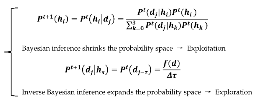
In making this choice, animals use the information of known experience regarding “this place” and move out toward the unknown. Bayesian inference can be considered a form of inference inspired by this kind of decision making. Bayesian inference is different from classical probability theory, and prior probability and posterior probability are introduced to change the probability space. Updating the prior probability by experience and changing the probability of the unused hypothesis to 0, Bayesian inference makes top-down decisions by shrinking the probability space. Recently, many experiments have reported that many animals, including humans, perceive the outside world by using Bayesian inference.

However, Bayesian inference that only shrinks the probability space is also a calculation procedure that identifies a concept of probability established on infinite attempts by using finite attempts. Through this process, known and unknown information are separated, and unknown information is discarded in an open environment. Here, there is no concept of time. The real environment does not stay the same but is always changing. In an unknown space, not only updating prior probabilities but also updating the likelihood of hypotheses is needed.

Therefore, inverse Bayesian inference is introduced as another form of inference [15,16,17,18,19]. Inverse Bayesian inference updates not only the probability of hypotheses but also the likelihood of hypotheses according to the latest input from the outside. In the process of searching for food resources, a system introducing both Bayesian and inverse Bayesian inference (BIB) needs to be constructed to solve the dilemma of exploration and exploitation. Inverse Bayesian inference, expanding the probability space, and Bayesian inference, shrinking the probability space, can correspond to exploration and exploitation [20].

In addition, we implemented a model of inhibited actin polymerization inspired by Sabil Huda et al., 2018 [6], and investigated the change in the foraging pattern. In this study, we built a model of amoebae imitating metastatic cancer cells and implemented BIB Inference as a decision maker for foraging. Our motivation is to explain the mechanism of general amoebic motility through describing the mechanism of cancer metastasis. Previous studies [6] have shown that when cancer cells metastasize, they do a Lévy walk. In this study, we use the Lévy walk observed as a mechanism for cancer cells to metastasize as a starting point, and compare it with the experiments of Sabil Huda et al. in which they applied various inhibitory conditions to cancer cells and investigated the changes in behavior related to the Lévy walk. We will show that Bayesian and inverse Bayesian inference play an important role in understanding the behavior of the Levy walk. We compared the Bayesian inference model, BIB inference model and random walk model and investigated the relationships among them.

This paper is structured as follows: In Section 2, we describe the algorithm of the amoebic foraging model and random walk as well as Bayesian and BIB inference. In Section 3, we show the results of the experiments. Finally, we compare these results in Section 4, and we state our conclusions in Section 5.

2. Materials and Methods

2.1. Amoebic Model

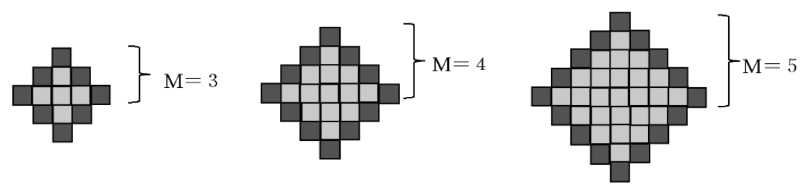
In this study, we implemented Bayesian and inverse Bayesian inference in an amoebic model [21,22,23] and constructed a model of metastatic cancer cells. The initial state of the amoeba is square with boundary points (dark gray grid points) at each boundary (Figure 1). The size of the amoeba is defined as the scale M, which is the distance from the center of the amoeba to the boundary. A dark gray grid point is the surface of the cell, and a light gray grid point is the internal area of the cell filled with plasma, where all grid points are sustained by actin tissue.

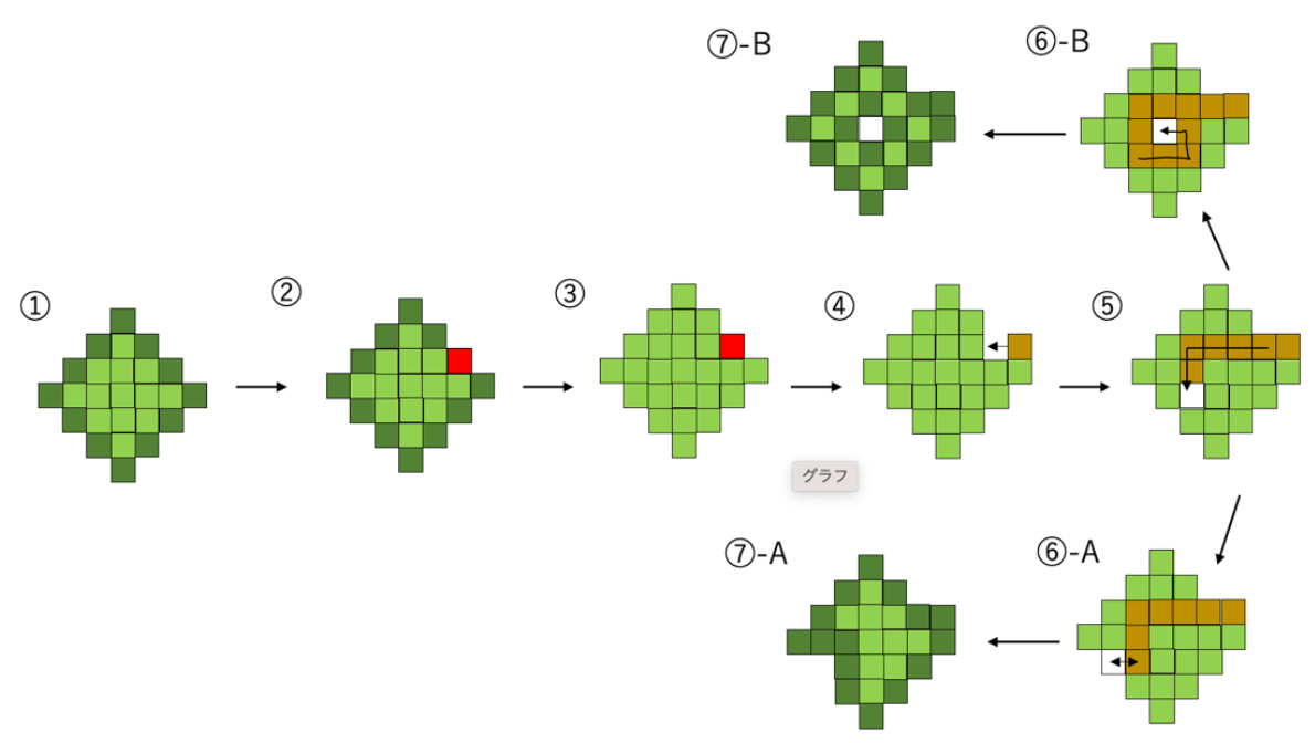
Amoebic motility is modeled by the following process (In Figure 2): First, one of the boundary points is chosen (Figure 2-②). Then, boundary glid points (dark green) and internal glid points (light green) are not distinguished to each other and are ready to be replaced. (Figure 2-③) Next, the external grid point invades the amoeba from the outside and replaces a glid point chosen in the process ② (Figure 2-④). This external grid point transfers to inside the cell, exchanging its position with each grid point that forms the amoeba body (Figure 2-⑤). At this time, the trail of external grid point is memorized, each cell replaced once (yellow glid points) cannot be replaced anymore until the external glid point finishes their movement. Finally, the white grid point is either deemed to be discharged at a place exposed in three directions (Figure 2-⑥A) or settles inside the cell surrounded by its own trails (Figure 2-⑥B). In both cases, all the glid points that are not surrounded by the other four glid points in the direction up, down, left, and right become boundary points (Figure 2-⑦). Although the external grid point’s transfer causes the shape of the cell to change, the overall size of the amoeba does not change, and its volume is preserved because each grid has just exchanged at its position.

The exchange between a white grid point and green grid point corresponds to the hollow space, which generates an outflow of surrounding plasma when the depolymerization of actin filaments occurs on the surface of the cell. After this exchange, plasma drift is expressed by grid points changing places where actin tissues are broken. The white grid points that transfer inside the cell avoid their own trails. This means that the plasma that drifts into a space is not easily broken because of rapid repolymerization.

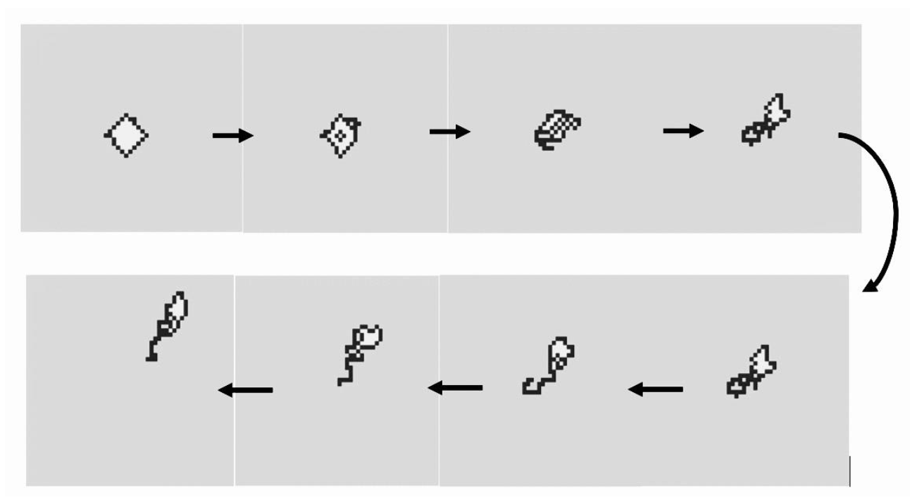
Thus, amoebae change their shape sequentially for each invasion of a white grid point. Although white grid points transfer inside a cell randomly, avoiding their own trails causes discharge in the opposite of the invading direction. This enables amoebae to move in the direction from which the white grid point invaded (Figure 3). Therefore, inference about the direction from which the white grid point invaded represents foraging for food resources.

In this study, the frequency of white grid point invasion was defined as 2M times each size of the amoeba model. The white grid point invades 8 times if M = 4 and 12 times if M = 5 for every inference.

2.2. Bayesian and Inverse Bayesian Inference

Here, we construct an amoebic foraging model that implements Bayesian inference, inverse Bayesian inference, and random walks. Bayesian inference is a statistical inference method using prior information acquired from past data. From conditional probability P(A|B); that is, P(A|B) = P(A,B)/P(B), the Bayesian formula is obtained by the following:$P^t\left(h_i|d_j\right) =\frac{P^t(d_j|h_i)P^t(h_{i })}{P^t(d_{i })}$ where h represents hypothesis and d is direction selection. Both h-hypothesis and d-direction have four patterns that are simply up, down, left, and right. In other words, each h and d has four parameters, which are marked with 0~3 in the program. This is described in further detail in Figure 4. In addition, the probability of choosing a data point $P^t\left(d_j\right)$ derived by adding the probabilities of choosing $d_j$ from all hypotheses is expressed by: $P^t\left(h_i|d_j\right) =\frac{P^t(d_j|h_i)P^t(h_{i })}{P^t(d_{i })}$.

By assigning these equations,

$$P^t\left(h_i|d_j\right) =\frac{P^t(d_j|h_i)P^t(h_{i })}{{{\displaystyle \sum }}_{k=0}^3{P}^t(d_j|h_k)P^t(h_{k })},$$

(1)

is obtained. We use (1) as the basic formula of Bayesian inference. In Bayesian inference, the probability of a hypothesis $P\left(h\right)$ is called the prior probability, and the probability of the hypothesis updated by experience is called the posterior probability. The idea of Bayesian inference is the process of using the posterior probability to obtain the next prior probability.

$$P^{t+1}\left(h_i\right) =P^t\left(h_i|d_j\right).$$

(2)

In BIB inference, after the application of (1) and (2), a hypothesis of lower probability is chosen randomly and assigned as $P\left(d_i\right)$, from t to $t-\tau$, to each likelihood and then updated. The probability of $d_i$ approximated from the empirical frequency is $P\left(d_j,\tau \right)$. Inverse Bayesian inference is expressed by:

$$P^{t+1}\left(d_j|h_s\right) =P^t\left(d_j,\tau \right).$$

(3)

The amoeba model determines the direction of t + 1 by using the posterior probability P(h|d) and the likelihood. τ is a value that refers to the number of times that the amoeba chose a direction in the past. Note that expressions (2) and (3) constitute an explicit symmetry structure such as a pair of P(h) = P(h|d) and P(d|h) = P(d). In previous models based on Bayesian inference, only P(h) = P(h|d) is implemented, and then the probability space is perpetually contracted dependent on the system’s own experience. It results in rapid approach of the steady state. In contrast, in our model, P(d|h) = P(d), which is called inverse Bayesian inference, is also added. That formula is defined to satisfy the symmetrical structure, by replacing d with h and h with d. Additionally, P(d|h) = P(d) reveals expansion of the probability space and entails cancelling the steady state. The symmetry implemented by a pair of P(h) = P(h|d) and P(d|h) = P(d) can balance contraction and expansion of the probability space under a disturbed environment.

In the amoeba model, for any h,

$$P^t\left(h_{max}\right) >P^t\left(h\right).$$

(4)

We choose a hypothesis $h_{max}$ satisfying (4), and for any d,

$$P^t\left(d_{max}|h_{max}\right) >P^t(d|h_{max}).$$

(5)

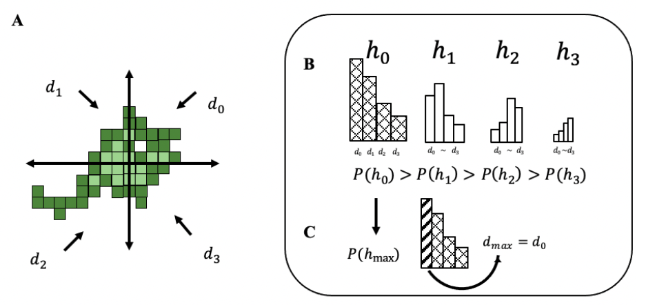
We randomly choose $d_{max}$ satisfying (5). Regarding the center of gravity of the amoeba body as the origin, with quadrants 1–4 corresponding to each d = 0~3, the amoeba chooses a boundary point relative to quadrants $d_{max}+1$, and the white grid point is allowed to invade. Finally, amoebic motility implementing Bayesian inference is constructed. Figure 5 shows both algorithms simply.

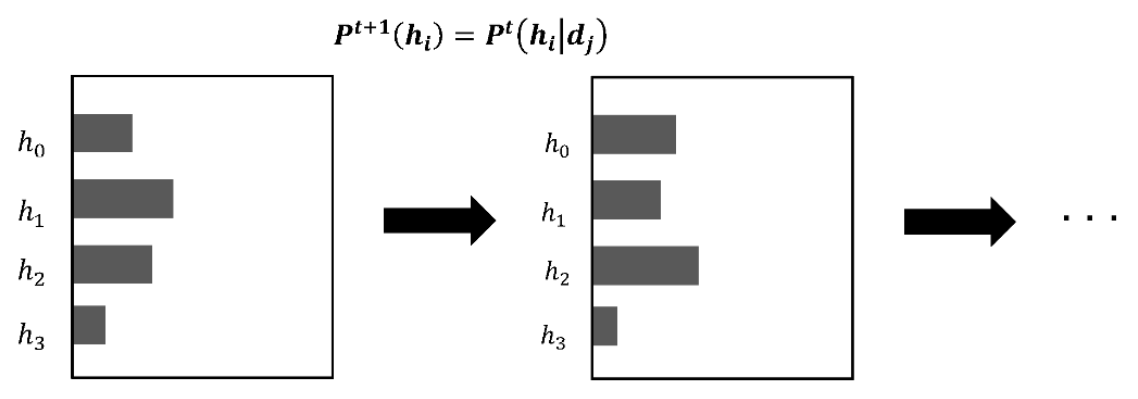
In Bayesian inference, the prior probability of the hypothesis is updated (Figure 6). A hypothesis is defined by its likelihood based on the data, but Bayesian inference does not change the hypothesis itself. Only the probability of the hypothesis is changed.

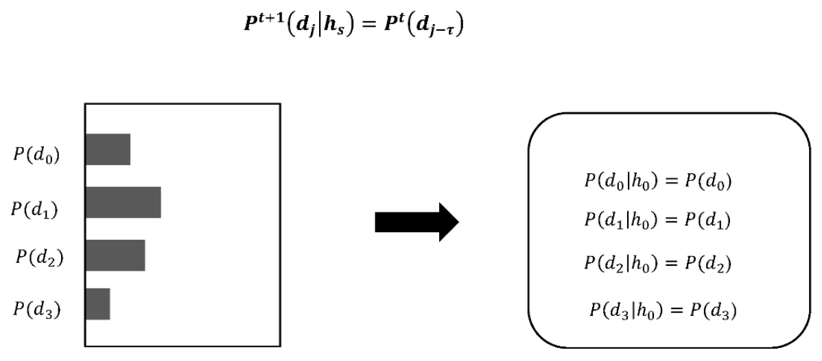
In inverse Bayesian inference, the past data of τ direction choices are referred to, and the likelihood is updated (Figure 7). The algorithm is shown in Figure 6. BIB inference makes decisions by applying both Bayesian and inverse Bayesian inference alternately.

Moreover, we added a new model of BIB amoeba. The original model determines the direction by choosing $d_{max}$ acquired from the changing probability of the hypothesis based on the latest input information through the BIB inference process. This means that actin polymerization and depolymerization are perfectly controlled in real amoebae. On the other hand, the condition that actin polymerization is controlled by a chemical inhibitor can be implemented as a process in which the $d_{max}$ acquired by Bayesian inference does not work, and the direction is therefore determined randomly. Thus, a new model is added, which ignores inference results with a probability of ν, where ν is the probability of randomness in choosing the direction of quadrants 1–4; that is, $d_{max}$ is used with a probability $1-\nu$. It is expected that random walk-like motility will appear because inference does not work.

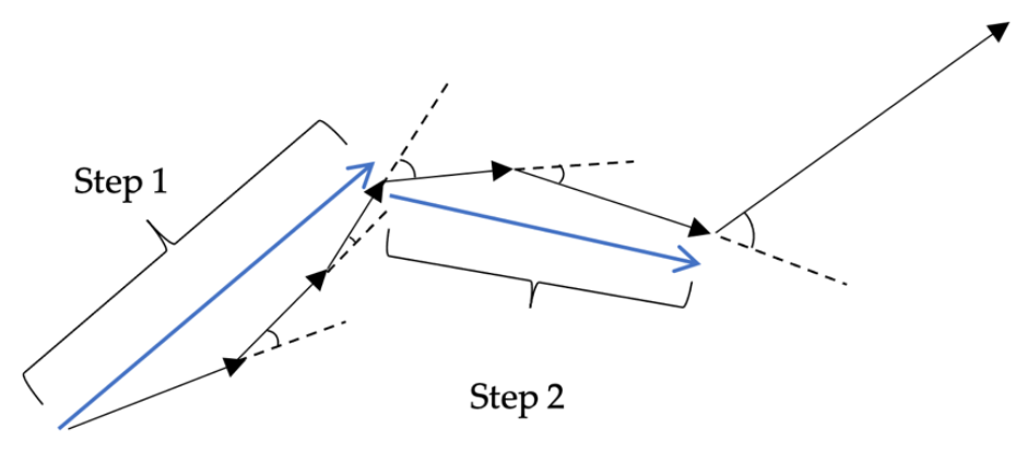
2.3. Analysis: Step Length

Step length is the length of straight-line movement in the foraging trail. The step length is calculated from the foraging data acquired in the experiment. Here, if the angle is formed by two continuous vectors acquired by two position coordinates updated by t = 10 is 40° or less, the distance is counted as one step (Figure 8).

2.4. AIC

We examined whether the step length distribution was a power law distribution or exponential distribution. Two probability density functions are given, one for the truncated power law distribution, f(x) = (μ − 1)/(x_min^{1 − μ} − x_max^{1 − μ})x^−μ, and the other for the exponential distribution, $f\left(x\right) =\lambda exp\left(-\lambda \left(x-xmin\right)\right)$, where x_min is determined by using Kolmogorov-Smirnov statistics and x_max is defined as the maximum value of the data. After best-fit exponents for the truncated power law () and the exponential distribution (λ) and log-likelihood are calculated, the AIC and Akaike weight for both models are calculated. Finally, the better-fitting model is determined based on the Akaike weight. We calculated the Akaike weight for the truncated power law distribution, $0.0\le wpl \le 1.0$, where the larger wpl is, the higher the likelihood of the truncated power law distribution is. In contrast, 1-wpl represents the likelihood for the exponential distribution.

In Section 3 if wpl is near 0, it is nearly an exponential distribution; if wpl is near 1, it is nearly a power law distribution.

3. Results

3.1. Experimental Condition of Foraging

An amoebic foraging model implementing random walks, Bayes and BIB was evaluated for each foraging pattern and step length distribution. In the random walk model, the entrance point is chosen randomly. In the Bayes and BIB models, amoebae forage randomly τ times to give the likelihood of prior probability. Each experiment is performed 50 times with $t=5000$. In our experiment, the initial values of the probability of the hypothesis and likelihood are given below (

Table 1. Initial value of hypothesis and likelihood.

	$d_0$	$d_1$	$d_2$	$d_3$
$h_0$	0.4	0.2	0.2	0.2
$h_1$	0.2	0.4	0.2	0.2
$h_2$	0.2	0.2	0.4	0.2
$h_3$	0.2	0.2	0.2	0.4

).

3.2. Step Length Distribution and Foraging Pattern

We show the graph of the relationship between the step length and its frequency and the pattern of foraging in each model. The trendlines are calculated by both a power law function and exponential function. In the graph, the blue curve is an exponential curve, and the green curve is a power law curve. In addition, the graph is a double logarithmic chart.

3.3. Details of the Distribution

We show the coefficient μ of the power distribution and the coefficient λ of the exponential distribution obtained by the approximation of each experimental data point.

Table 2. Results of each graph.

	μ	λ	wpl
Random M6	2.644600	1.038069	0.00000
Bayes M6	2.287500	0.708772	1.00000
BIB M6 τ = 50	1.968700	0.297233	1.00000
BIB M6 τ = 75	2.114100	0.451981	1.00000
BIB M6 τ = 100	2.205200	0.529439	1.00000
BIB M6 τ = 200	2.407700	0.719001	1.00000
BIB M8 τ = 100	2.091800	0.451882	1.00000
BIB M4 τ = 100	2.051100	0.423548	1.00000

shows the data for random walk, Bayesian foraging, BIB foraging τ, and the size of amoeba M from bottom to top. wpl is a value that is 1 if the step length frequency distribution can be approximated as a power distribution by AIC and 0 if it can be approximated by an exponential distribution. When wpl = 1, the focus is on whether the value of the parameter μ related to the power function is close to 2, and when wpl = 0, the focus is on whether the value of the parameter λ related to the exponential function is close to 1. In Table 2, μ is close to 2 for BIB M6, τ = 50 and 75, and M4 and 8, τ = 100, suggesting a Lévy walk. On the other hand, Random M6 is close to λ = 1 at wpl = 0, so it closely approximates the exponential distribution. In addition, BIB M6, τ = 200, shows a dissociation from μ = 2.407700 and μ = 2.

4. Discussion

4.1. Comparison of Random, Bayesian and BIB Foraging

4.1.1. Random Walk

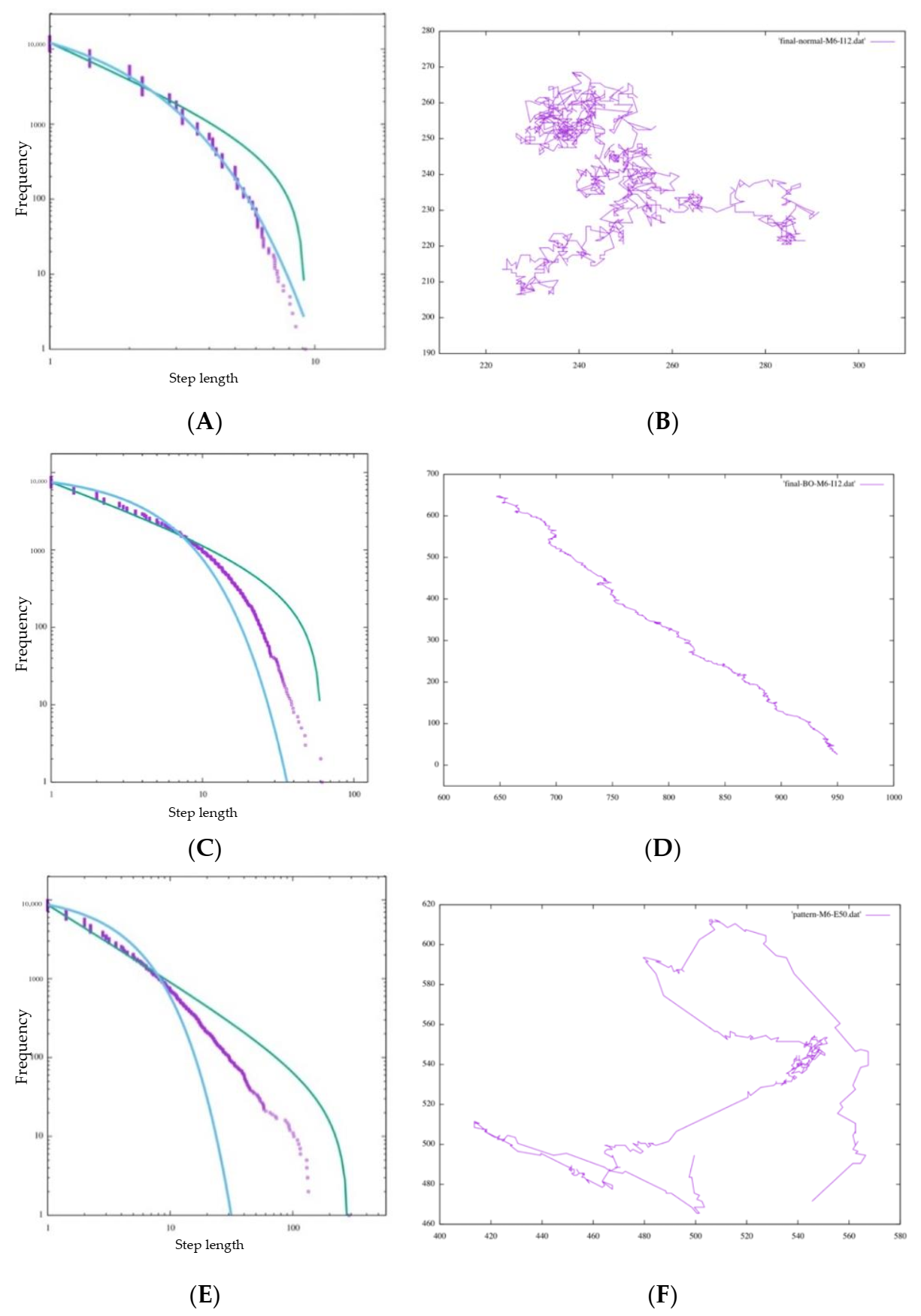
In Figure 9A, the step length distribution of the random walk seems to be close to the exponential trendline. Additionally, in the foraging pattern example in Figure 9B, the random walk is composed of many short steps and turns, and a long step characterizing a Levy walk does not appear, which means that the cell cannot search in a large space. In Table 2, AIC-wpl = 0.00000 indicates that the step length distribution is a random walk. In addition, near λ = 1, the distribution is better approximated by an exponential function.

4.1.2. Bayesian Foraging

We consider Bayesian foraging as well. In Figure 9C, even though the distribution does not fit an exponential function better than a random walk, it is far from a power law distribution. On the other hand, AIC;wpl = 1.00000 indicates that it is approximated well by a power law distribution. However, the foraging pattern in Figure 9D confirms that the cell occasionally changes its traveling direction and forages in only one direction.

This heavily depends on the initial likelihood of Bayesian inference. In Bayesian inference, each of four initial likelihoods, which are the hypotheses with the highest probability in each direction, are configured. Because Bayesian inference does not update its likelihood based on experience as inverse Bayesian inference does, once the experiment starts, the probabilities of hypotheses $h_0\sim h_3$ soon bias one of the directions comparatively, and the cell, unable to move in the remaining three directions, shows ballistic movement in one direction. This can also be seen in the foraging pattern example in Figure 9E. This means that the cell keeps searching without exploiting resources in the current environment or balancing exploration and exploitation. However, from the perspective of the animal action strategy, this foraging bias in one direction without widespread searching cannot be regarded as an efficient foraging pattern and does not have scale-free characteristics. In this context, we judge that Bayesian foraging does not fit the other features of the Lévy walk.

4.1.3. BIB Foraging

We consider Bayesian foraging as well. As shown in Figure 9E, the step length distribution of BIB foraging is nearly a power law distribution, and the models of any τ and M show wpl = 1.00000 and a μ of approximately 2 and can be approximated by a power law distribution. Comparing the difference of the maximum step length with the size of M, each distribution satisfying the power-law distribution indicates scale-free characteristics. In fact, μ is often 2 for many animals, so it can be said that this foraging model of BIB inference replicates the Lévy walk. At first glance, it appears that the data do not fit well on the line of the power distribution on the graph, but we judged the goodness of fit by the value of µ, which is an evaluation value of the Akaike criterion. Regarding the comparison of BIB and Bayes only, we evaluate Lévy walk-like movements with not only AIC but also trail patterns comprehensively.

In Figure 9F, there are both ballistic movements and random movements. These can be substituted with exploration and exploitation. Random movement is an exploitative behavior composed of many short steps for the purpose of obtaining food resources, and ballistic movement is exploratory behavior that contains a few long steps for the sake of finding potential feeding grounds. Considering the above, we can say that the random walk is dedicated to exploitation and the Bayes Only model is dedicated to exploration. Of course, both exploration and exploitation are important in the foraging behavior of animals, but it is impossible for animals to behave well if they are biased toward one or the other. The BIB model, on the other hand, can be said to have a good balance between exploration and exploitation in that it supports exploration by repeating exploitation for a certain period of time in one place and periodically taking long steps to another remote place.

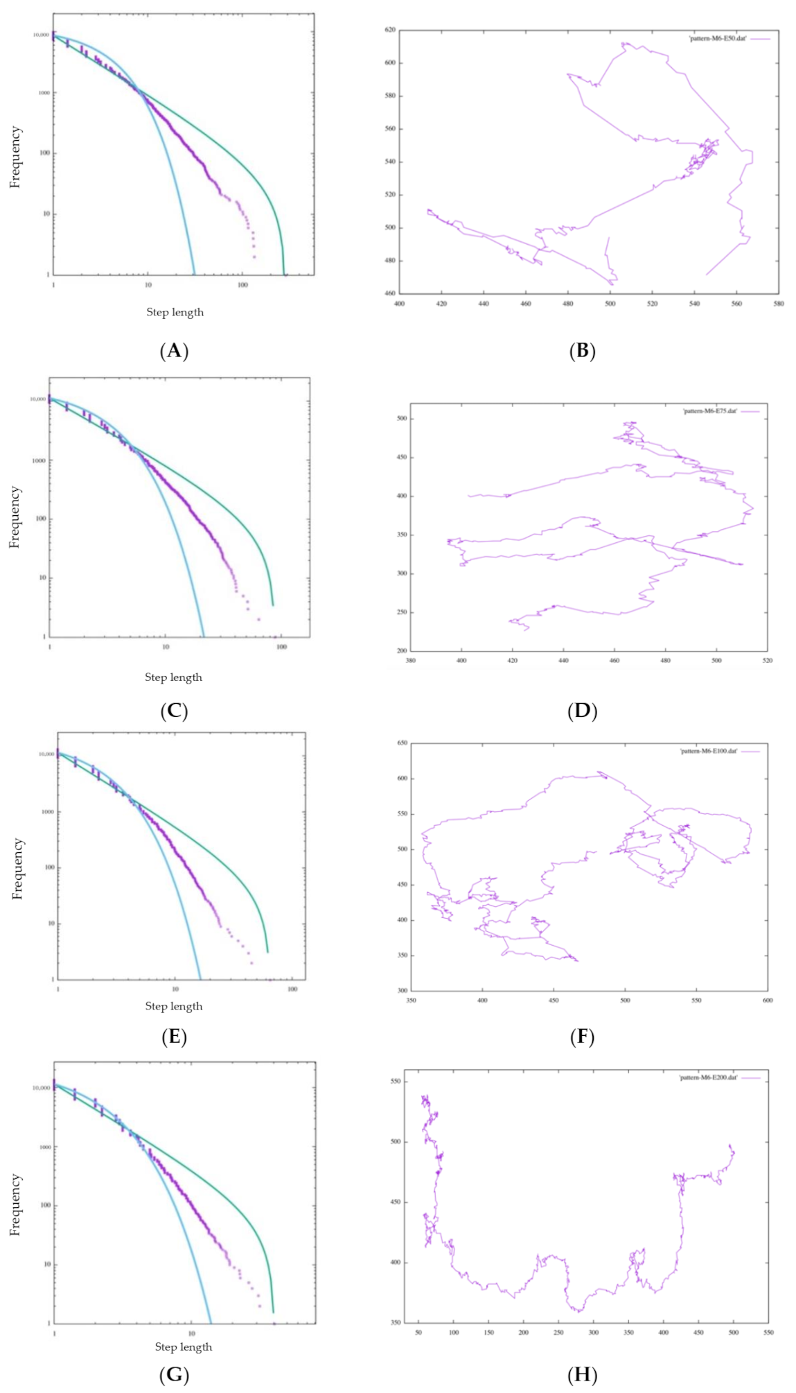
4.2. Comparison of BIB Foraging by $\tau$

In BIB foraging, it was confirmed that the Lévy walk was performed in all models of $\tau =50, 75, 100, 200$, but it was also found that the behavior changed depending on the value of τ. Comparing Figure 10, from $\tau =50$ to $\tau =200$, the linearity of the distribution increases, but the maximum step length tends to decrease.

At $\tau =200$, $\mu =2.4$and the ideal value of $\mu =2$ are slightly dissociated. This can be explained by the relationship between the value of τ and the update of the likelihood by inverse Bayesian inference. The magnitude of $\tau$ is a measure of how well the amoebae remember their own course choices. In the BIB model, before the start of BIB walking, the grid was randomly invaded a number of times $\tau$. Therefore, past data was referred to immediately after the start of walking in the BIB model, and the larger the value of τ is, the more random equality is indicated. That is, the larger the value of τ is, the more evenly distributed the likelihood updated by inverse Bayesian inference is in the four directions, and conversely, the smaller the value of τ is, the larger the bias in the four directions.

Therefore, a small value of $\tau$ is greatly affected by a small bias, and suddenly, a very long step appears while greatly changing the probabilities of the four hypotheses. Therefore, the linearity of the power distribution is somewhat impaired, but a wider range can be searched. On the other hand, if the value of $\tau$ is large, the likelihood is updated stably, and the surroundings are searched “moderately”. Therefore, the linearity of the exponentiation distribution is more stable than that of a small $\tau$, but the maximum step length is small, and a wider range of searching cannot be performed.

In an unknown space, referring to all past data and memories and taking an absolute view of them cannot enable a response to completely unknown events that have never been experienced before. Unexpected things always happen in the real world. It is a daily occurrence that events do not correspond to any past data. In this case, it is important not to stick to past data too closely in order to accept something completely unknown. The magnitude of the value of $\tau$ is considered to correspond to this idea.

If $\tau$is too small, it will be affected by the bias of the latest data too greatly, and the hypothesis will be determined quickly. On the other hand, if τ is too large, it approaches a random walk with an exponential distribution. It is difficult to draw a conclusion in this experiment, but τ most likely has an optimal value under certain conditions such as the individual and the environment. If $\mu =2.00000$ is the ideal setting for τ, it is reasonable to consider that there is an optimal value between $\tau =50$ and 75 in this experiment.

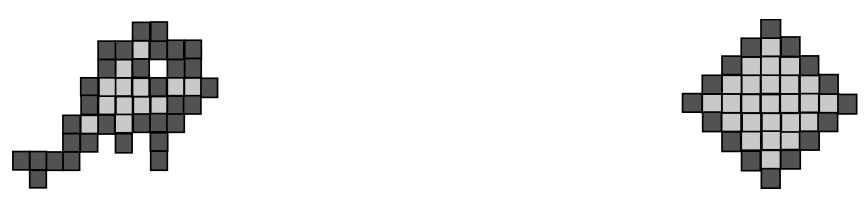
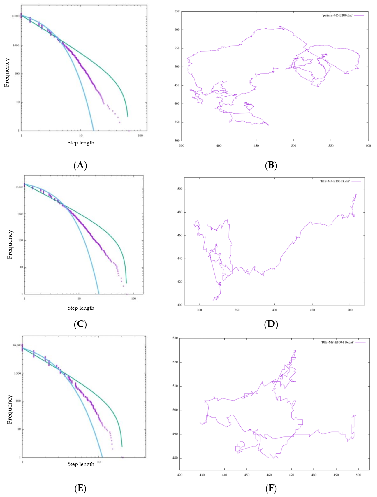
4.3. Comparison of Amoebae by Size

In our study, experiments with amoeba models of different sizes (M = 4, 6, 8) were conducted. This time, in each direction decision, white grid points invade a number of times twice as large as M. Although in the initial state of square amoeba, the number of grids on each side is theoretically √2 M in each direction, it changes its shape for each invasion and increases in thickness more than a straight line (Figure 11).

Therefore, considering this increase, this value is configured. In Table 2, all amoebas satisfy $wpl=1.00000$ and $\mu$is nearly 2, indicating Lévy walk behavior. This may be one of the reasons why BIB inference is effective in exploration regardless of the cell size and the scale of the animal itself. On the other hand, the value of this number of invasions is arbitrary, so it should be confirmed in another experiment how many invasions are appropriate for each size. In fact, when Figure 12A,C,E are compared, the maximum step length (right end of the horizontal axis) is significantly smaller than for the other sizes of M, such as when $M=8$. Additionally, this time, the number of invasions was set to be proportional to the value of M in relation to the height index of the side of the amoeba, but the movement of the amoeba itself was actually realized by repeating the movements of two cells for each invasion. Therefore, the value was set to be proportional to $M^2$, which is related to the number of grids in the area of the amoeba. Considering this, the most appropriate value was chosen according to the value of each M and the size of the amoeba.

4.4. Model Reproduction of Chemical Inhibitors

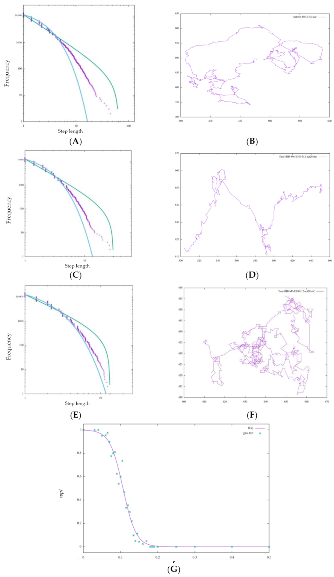
A clear difference was also seen depending on the value of ν. Figure 13G shows the change in $wpl$ with respect to a continuous change in ν. The value of $wpl$ begins to decrease as the estimation of the model that was performing a Lévy walk without inhibition becomes 5% (ν = 0.05) randomly; when it reaches 20% (ν = 0.2), wpl becomes 0.00000, and it can be seen that wpl decreases sharply near ν = 0.05 to 0.2. Looking at the walking patterns in Figure 13B,D,F, the ballistic movement disappears as ν increases, and the behavior approaches random walk-like behavior from Lévy-walk-like behavior.

For the amoebae, the walking pattern changed from a Lévy walk to random walk by inhibiting the BIB inference estimation result by 20%. This is in line with Sabil Huda’s experimental results showing that the survival strategy of metastatic cells is impeded and effective exploratory behavior is not possible. What is important to note about the results of this experiment is that the interference with the BIB inference mechanism, which may be involved in the decision making regarding the directional selection of the Lévy walk, produced results similar to the fact that actual cancer cells changed from Lévy walk behavior to a random walk when their behavior was interfered with by actin inhibitors, as observed in previous studies.

Recently, active inference or free energy theorem plays an important role in describing not only human cognition but also biochemical reaction networks [24,25,26]. It implies that cognitive system usually uses Bayesian inference in making decision, and that the probability of hypothesis is replaced by the conditional probability of hypothesis under a specific data (i.e., the system’s own experience). It implies that a system removes what is unexperienced in possible candidates, and that the computation to compare possible states is accelerated in decision making. Compacting a set of possible states is ubiquitously found in various biological system, such as biochemical network and neural network. It is shown that biological real networks are very sparse, compared to complete network [27,28]. However, it is overlooked that even a sparse network is perpetually changed through time, not to be fallen into the steady state. Since Bayesian inference realizes only the decision making at the representative case, the process of decision making is falling into the steady state. However, real process is perpetually changed dependent on the environment. Thus, it entails modification or cancellation of the likelihood of hypothesis. To implement such modification or cancelation, we here implement inverse Bayesian inference, and the likelihood of a hypothesis is perpetually modified dependent of empirical data. Lévy walk is a typical foraging behavior of animals of which animals show both stationary and non-stationary behavior. In terms of foraging behavior, stationary behavior in a closed environment reveals random walk, while non-stationary behavior reveals ballistic movement escaping from the closed environment. A mixture of stationary and non-stationary foraging results in a long-tailed distribution of step-length, which is called the Lévy walk. By focusing on the definition of Lévy walk, it is reasonable that coexistence of Bayesian and inverse Bayesian (BIB) inference is consistent with Lévy walk. Since foraging behavior results from searching for food, a specific distribution of food can enable Lévy walk in the form of steady state. It is consistent with our results in which even only-Bayesian inference can enable power law distribution. The question arises whether coexistence of stationary and non-stationary behavior in opened environment can be explained only by BIB inference. In other words, power law distribution in an opened environment can be explained only by BIB inference, and that might be true for Lévy walk. In our research, step length distribution obtained not only by BIB inference but by only-Bayesian inference shows power law distribution, where the exponent of the power law by BIB inference is closer to the value of 2.0, representing a typical Lévy walk. This suggests that true Lévy walk is consistent with only BIB inference.

5. Conclusions

The amoeba model of BIB foraging was able to replicate a cancer metastasis and Lévy walk at the same time. We found that both BO and BIB models behave differently from random walk, and that Bayes only is not sufficient for exploratory behavior. Then, the difference by the size of the amoeba was also clearly shown. Differences in the amount of memory for the direction of travel were also found to cause changes in the walking pattern. The results suggest that the amount of memory greatly affects the exploration of unknown space, and that it is not good to have too little or too much memory. In the model that mimicked the experiment in which an inhibitor of actin polymerization was applied to cancer cells, we obtained the result that by inhibiting the BIB inference of the BIB model that was performing the Levy walk, its gait pattern continuously faded, which also corresponded to the results of the mimicked experiment. This experiment may have shown that BIB inference is an effective means of exploration in an unknown environment. It also showed that BIB inference is related not only to humans and other large animals but also to the cellular level of the microscopic world. It was also confirmed that BIB inference behaves differently from the Bayesian inference-only model in updating not only the prior probabilities but also the likelihood that the hypothesis will improve the responsiveness to the unknown. More detailed research on the Lévy walk will continue for various agents, environments and fields. Further application of BIB inference in the fields of biology and cognitive science is expected.