Stationary Distribution and Extinction in a Stochastic SIQR Epidemic Model Incorporating Media Coverage and Markovian Switching

Abstract

This paper is concerned with the dynamic characteristics of the SIQR model with media coverage and regime switching. Firstly, the existence of the unique positive solution of the proposed system is investigated. Secondly, by constructing a suitable random Lyapunov function, some sufficient conditions for the existence of a stationary distribution is obtained. Meanwhile, the conditions for extinction is also given. Finally, some numerical simulation examples are carried out to demonstrate the effectiveness of theoretical results.

1. Introduction

Mathematical models are important tools to study the transmission mechanism of infectious diseases. The control and elimination of infectious diseases have become urgent problems to solve. From then on, epidemic models with different influencing factors are proposed by many reseachers. These influencing factors include immunity, delay, noise, incubation, saturated incidence rate, media coverage, information spreading of awareness, information spreading and disease diffusion, vaccination strategies and so on [1,2,3,4,5,6,7,8,9,10,11]. For example, Ariful Kabir et al. [1] studied a SIR epidemic model with information spreading of awareness.

When an infectious disease appears in local areas, the most important work of the disease control department is to control the spread of this disease. One of the effective preventive measures is to release the relevant prevention knowledge to people through the media mass media including TV, radio broadcast, network, newspaper and so on. After obtaining relevant prevention knowledge through mass media [12,13,14], people usually take some measures to avoid infection. Tchuenche et al. [15] incorporated a nonlinear function of the number infective individuals in transmission term to study the effects of media coverage on the transmission dynamic. This nonlinear function can be expressed in the following form

$$\begin{array}{c}\hfill f\left(t\right)={\beta }_1-\frac{{\beta }_{2}I}{m+I}.\end{array}$$

where ${\beta }_1$ is the contact rate before media alert, the term ${\beta }_{2}I/(m+I)$ measures the effect of reduction of the contact rate when infectious individuals are reported in the media. The half-saturation constant $m>0$ reflects the impact of media coverage on the contact transmission and ${\beta }_1\ge {\beta }_2>0$.

As is well known, epidemic models are affected inevitably by external environmental noise, which is a very important component in the ecosystem. In order to describe the influence of external environmental noise on infectious diseases, many authors incorporated stochastic perturbation into the epidemic models [16,17,18,19,20]. For example, Qi et al. [19] studied a stochastic SIQS epidemic system. Some sufficient conditions for periodic solution and ergodic stationary distribution of the disease are obtained by using the Khasminskii’s theory. Liu et al. [17] introduced the media coverage and the environment noise into a SIRS epidemic model with saturated incidence rate by perturbing the disease transmission coefficient $\beta$. They gave a detailed analysis on the existence of ergodic stationary distribution of the disease. Inspired by the above works, one proposes a stochastic SIQR model

$$\begin{array}{c}\hfill \left\{\begin{array}{ccc}dS\left(t\right)\hfill & =\hfill & \left[\mathsf{\Lambda }\left(t\right)-\left({\beta }_1\left(t\right)-\frac{{\beta }_2\left(t\right)I\left(t\right)}{m\left(t\right)+I\left(t\right)}\right)\frac{S\left(t\right)I\left(t\right)}{N}-\mu \left(t\right)S\left(t\right)\right]dt+{\sigma }_1\left(t\right)S\left(t\right)d{B}_1\left(t\right),\hfill \\ dI\left(t\right)\hfill & =\hfill & \left[\left({\beta }_1\left(t\right)-\frac{{\beta }_2\left(t\right)I\left(t\right)}{m\left(t\right)+I\left(t\right)}\right)\frac{S\left(t\right)I\left(t\right)}{N}-(\mu \left(t\right)+\alpha \left(t\right)+\delta \left(t\right)+\gamma \left(t\right))I\left(t\right)\right]dt\hfill \\ & & +{\sigma }_2\left(t\right)I\left(t\right)d{B}_2\left(t\right),\hfill \\ dQ\left(t\right)\hfill & =\hfill & \left[\delta \left(t\right)I\left(t\right)-\left(\mu \right(t)+\alpha (t)+ϵ(t\left)\right)Q\left(t\right)\right]dt+{\sigma }_3\left(t\right)Q\left(t\right)d{B}_3\left(t\right),\hfill \\ dR\left(t\right)\hfill & =\hfill & \left[\gamma \left(t\right)I\left(t\right)+ϵ\left(t\right)Q\left(t\right)-\mu \left(t\right)R\left(t\right)\right]dt+{\sigma }_4\left(t\right)R\left(t\right)d{B}_4\left(t\right).\hfill \end{array}\right.\end{array}$$

(1)

where $S,I,R$ denote the number of susceptible, infective and removed, respectively, Q denotes the number of quarantined, $N=S+I+Q+R$ denotes the number of total population individuals. The parameter $\mathsf{\Lambda }$ denotes the recruitment rate of S corresponding to births and immigration, $\mu$ denotes the natural death rate, $\gamma$ and $ϵ$ are the recover rates from groups $I,Q$ to R, $\delta$ represents the removal rate from I, $\alpha$ denotes the disease-caused death rate of I and Q. All parameters are assumed to be nonnegative. $B_i\left(t\right)(i=1,2,3,4)$ are independent Brownian motions and ${\sigma }_i\left(t\right)(i=1,2,3,4)$ are the coefficients of the effects of stochastic perturbations. The functions $\mathsf{\Lambda }\left(t\right),{\beta }_1\left(t\right),{\beta }_2\left(t\right),m\left(t\right),\mu \left(t\right),\alpha \left(t\right),\delta \left(t\right),\gamma \left(t\right),ϵ\left(t\right)$ and ${\sigma }_i\left(t\right)(i=1,2,3,4)$ are positive and continuous functions with periodic T.

In addition to the white noise, the spread of infectious diseases may also be disturbed by telegraph noise which can lead to the system to switch from one environmental regime to another [21,22,23]. The switching between environmental regimes is usually memoryless and the waiting time of switching obeys exponential distribution [21]. Thus the regimes switching can be described by a continuous-time Markov chain ${\left(r\left(t\right)\right)}_{t\ge 0}$ taking values in a state space $\mathcal{M}=\{1,2,\cdots N\}$. If one considers the impact of the media coverage and the regime switching on the spread of infectious diseases, (1) can be changed to

$$\begin{array}{c}\hfill \left\{\begin{array}{ccc}dS\left(t\right)\hfill & =\hfill & \left[\mathsf{\Lambda }\left(r\left(t\right)\right)-\left({\beta }_1\left(r\left(t\right)\right)-\frac{{\beta }_2\left(r\left(t\right)\right)I\left(t\right)}{m\left(r\right(t\left)\right)+I\left(t\right)}\right)\frac{S\left(t\right)I\left(t\right)}{N}-\mu \left(r\left(t\right)\right)S\left(t\right)\right]dt+{\sigma }_1\left(r\left(t\right)\right)S\left(t\right)d{B}_1\left(t\right),\hfill \\ dI\left(t\right)\hfill & =\hfill & \left[\left({\beta }_1\left(r\left(t\right)\right)-\frac{{\beta }_2\left(r\left(t\right)\right)I\left(t\right)}{m\left(r\right(t\left)\right)+I\left(t\right)}\right)\frac{S\left(t\right)I\left(t\right)}{N}-(\mu \left(r\left(t\right)\right)+\alpha \left(r\left(t\right)\right)+\delta \left(r\left(t\right)\right)+\gamma \left(r\left(t\right)\right))I\left(t\right)\right]dt\hfill \\ & & +{\sigma }_2\left(r\left(t\right)\right)I\left(t\right)d{B}_2\left(t\right),\hfill \\ dQ\left(t\right)\hfill & =\hfill & \left[\delta \left(r\right(t\left)\right)I\left(t\right)-\left(\mu \right(r\left(t\right))+\alpha (r\left(t\right))+ϵ(r\left(t\right)\left)\right)Q\left(t\right)\right]dt+{\sigma }_3\left(r\left(t\right)\right)Q\left(t\right)d{B}_3\left(t\right),\hfill \\ dR\left(t\right)\hfill & =\hfill & \left[\gamma \left(r\right(t\left)\right)I\left(t\right)+ϵ\left(r\right(t\left)\right)Q\left(t\right)-\mu \left(r\right(t\left)\right)R\left(t\right)\right]dt+{\sigma }_4\left(r\left(t\right)\right)R\left(t\right)d{B}_4\left(t\right).\hfill \end{array}\right.\end{array}$$

(2)

For any $k\in \mathcal{M}$, the parameters $\mathsf{\Lambda }\left(k\right),{\beta }_1\left(k\right),{\beta }_2\left(k\right),m\left(k\right),\mu \left(k\right),\alpha \left(k\right),\delta \left(k\right),\gamma \left(k\right),ϵ\left(k\right)$ and ${\sigma }_i\left(k\right)(i=1,2,3,4)$ are all nonnegative constants.

The objectives of this paper are as follows. In this paper, one will study the influence of media coverage on the spread of infectious disease by investigating a stochastic SIQR epidemic model incorporating media coverage. From a mathematical point of view, the existence of unique global positive solution of this stochastic system will be studied to show that the system is meaningful in biology. Then, in order to obtain the conditions for the disease to persist or extinct, one will study the existence of ergodic stationary distribution and the extinct condition of the disease.

The rest of the paper is organized as follows. Some lemmas used throughout this paper are presented in Section 2. In Section 3, the existence and uniqueness of global positive solution of system (2) are obtained. In Section 4, one verifies that there is an ergodic stationary distribution of the proposed system. In Section 5, one establishes sufficient conditions for extinction of system (2). In Section 6, two examples are given to illustrate theoretical results. In Section 7, the conclusion and discussion are given.

2. Preliminaries

In this section, one introduces some notations and lemmas. Let $(\mathsf{\Omega },\mathcal{F},\mathbb{P})$ be a complete probability space with a filtration ${\left\{{\mathcal{F}}_t\right\}}_{t\ge 0}$ satisfying the usual conditions. Suppose the generator $\mathsf{\Gamma }={\left({\gamma }_{ij}\right)}_{N\times N}$ is given by

$$\begin{array}{c}\hfill p\left(r(t+\delta )=j\mid r\left(t\right)=i\right)=\left\{\begin{array}{cc}{\gamma }_{ij}h+o\left(h\right),ifi\ne j,\hfill & \\ 1+{\gamma }_{ij}h+o\left(h\right),ifi=j,\hfill \end{array}\right.\end{array}$$

where $h>0$. Hence ${\gamma }_{ij}>0$ is the transition rate from i to j if $i\ne j$, while ${\sum }_{j=1}^m{\gamma }_{ij}=0$. Furthermore, suppose further that the Markov chain $r\left(t\right)$ is irreducible and has a unique stationary distribution $\pi =({\pi }_1,{\pi }_2,\cdots ,{\pi }_m)$ which can be determined by the equation

$$\begin{array}{c}\hfill \pi \Delta =0,\end{array}$$

(3)

subject to

$$\begin{array}{c}\hfill \sum _{i=1}^m{\pi }_i=1,{\pi }_i>0,\forall i\in \mathcal{M}.\end{array}$$

One assumes that the Markov chain $r\left(t\right)$ is independent of the Brownian motion $B\left(t\right)=(B_1\left(t\right),B_2\left(t\right),B_3\left(t\right),B_4\left(t\right))$. For any vector $f=\left(f\right(1),f(2),\cdots ,f(m\left)\right)$, $\widehat{f}={min}_{k\in \mathcal{M}}f\left(k\right),\breve{f}={max}_{k\in \mathcal{M}}f\left(k\right)$.

Let $\left(X\right(t),r(t\left)\right)$ be the diffusion Markov process satisfying the following equation

$$\begin{array}{c}\hfill dX\left(t\right)=b(X\left(t\right),r\left(t\right))dt+\sigma (X\left(t\right),r\left(t\right))dB\left(t\right),X\left(0\right)=x_0,r\left(0\right)=r,\end{array}$$

(4)

where $b(·,·):{\mathbb{R}}^n\times \mathcal{M}\to {\mathbb{R}}^n,\sigma (·,·):{\mathbb{R}}^n\times \mathcal{M}\to {\mathbb{R}}^{n\times n}$ and $D(x,k)=\sigma (x,k){\sigma }^{\mathrm{T}}(x,k)=\left(d_{ij}(x,k)\right)$. For each $k\in \mathcal{M}$, let $V(·,k)$ be any twice continuously differentiable function, the differential operator L of Equation (4) is defined by

$$\begin{array}{c}\hfill L(x,k)=\sum _{i=1}^n{b}_i(x,k)\frac{\partial V(x,k)}{\partial x_i}+\frac{1}{2}\sum _{i=1}^n{d}_{ij}(x,k)\frac{{\partial }^{2}V(x,k)}{\partial x_i\partial x_j}+\sum _{i=1}^m{\gamma }_{kl}V(x,l).\end{array}$$

Lemma 1.

(R. Lipster [24]) If the following conditions are satisfied

$\left(a\right)$${\gamma }_{ij}>0$, for any $i\ne j$;

$\left(b\right)$ for each $k\in \mathcal{M},D(x,k)=\left(d_{ij}(x,k)\right)$ is symmetric and satisfies

$$\begin{array}{c}\hfill \lambda \mid {\xi }^2\mid \le (D(x,k)\xi ,\xi )\le {\lambda }^{-1}\mid {\xi }^2\mid ,forall\xi \in {\mathbb{R}}^n,\end{array}$$

with some constant $\lambda \in (0,1]$ for all $x\in {\mathbb{R}}^n$;

$\left(c\right)$ there exists a nonempty open set $\mathcal{D}$ with compact closure, satisfying that, for each $k\in \mathcal{M}$, there is nonnegative function $V(·,k):{\mathcal{D}}^c\to \mathbb{R}$ such that $V(·,k)$ is twice continuously differential and that for some $\varrho >0$,

$$\begin{array}{c}\hfill LV(x,k)\le -\varrho ,(x,k)\in {\mathcal{D}}^c\times \mathcal{M}.\end{array}$$

Then $\left(X\right(t),r(t\left)\right)$ of system (2) is positive recurrent and ergodic. Namely, there exists a unique stationary distribution $\pi (·,·)$ such that for any Borel measurable function $f(·,·):{\mathbb{R}}^n\times \mathcal{M}\to \mathbb{R}$ satisfies

$$\begin{array}{c}\hfill \sum _{k=1}^m{\int }_{{\mathbb{R}}^n}\mid f(x,k)\mid \pi (dx,k)<\infty ,\end{array}$$

and

$$\begin{array}{c}\hfill \mathcal{P}\left(\underset{t\to \infty }{lim}\frac{1}{t}{\int }_0^{t}f(X\left(s\right),r\left(s\right))ds=\sum _{k=1}^m{\int }_{{\mathbb{R}}^n}\mid f(x,k)\mid \pi (dx,k)\right)=1.\end{array}$$

Lemma 2.

(Mao [25]) Let $N={\left\{N_t\right\}}_t\ge 0$ be a real-valued continuous local martingale vanishing $t=0$. Then

$$\begin{array}{c}\hfill \underset{t\to \infty }{lim}{\langle N,N\rangle }_t=\infty a.s.\Rightarrow \underset{t\to \infty }{lim}\frac{N_t}{{\langle N,N\rangle }_t}=0a.s.\end{array}$$

and also

$$\begin{array}{c}\hfill \underset{t\to \infty }{lim\; sup}\frac{{\langle N,N\rangle }_t}{t}<\infty a.s.\Rightarrow \underset{t\to \infty }{lim}\frac{N_t}{t}=0a.s.\end{array}$$

3. Existence and Uniqueness of the Global Positive Solution

By the similar arguments to those in Theorem 2.1 in [19,26], one can obtain the following theorem

Theorem 1.

For any initial value $(S\left(0\right),I\left(0\right),Q\left(0\right),R\left(0\right),r\left(0\right))\in {\mathbb{R}}_{+}^4\times \mathcal{M}$, there exists a unique solution $\left(S\right(t),I(t),Q(t),R(t),r(t\left)\right)$ of system (2) on $t>0$ and the solution remain in ${\mathbb{R}}_{+}^4\times \mathcal{M}$ with probability one, that is to say, $(S\left(t\right),I\left(t\right),Q\left(t\right),R\left(t\right),r\left(t\right))\in {\mathbb{R}}_{+}^4\times \mathcal{M}$ for all $t\ge 0$ a.s.

Proof. 

Note that the coefficients of the model $\left(1.4\right)$ are locally Lipschitz conditions, then for any given initial value $(S\left(0\right),I\left(0\right),Q\left(0\right),R\left(0\right),r\left(t\right))\in {\mathbb{R}}_{+}^4\times \mathcal{M}$, there ia a unique positive local solution $\left(S\right(t),I(t),Q(t),R(t),r(t\left)\right)$ on $t\in [0,{\tau }_e)$, where ${\tau }_e$ is the explosion time. To demonstrate that this solution is global, one only need to prove that ${\tau }_e=\infty$ a.s.

Let $k_0>0$ be sufficiently large for any initial value $S\left(0\right),I\left(0\right),Q\left(0\right)$ and $R\left(0\right)$ lying within the interval $[1/k_0,k_0]$. For each integer $k\ge k_0$, define the following stopping time

$$\begin{array}{c}\hfill {\tau }_k=inf\left\{t\in [0,{\tau }_e):min\{S\left(t\right),I\left(t\right),Q\left(t\right),R\left(t\right)\}\le \frac{1}{k}ormax\{S\left(t\right),I\left(t\right),Q\left(t\right),R\left(t\right)\}\ge k\right\}\end{array}$$

where one sets $inf\varnothing =\infty$ (as usual ∅ denotes the empty set). Clearly, ${\tau }_k$ is increasing as $k\to \infty$. Let ${\tau }_{\infty }={lim}_{k\to \infty }{\tau }_k$, hence ${\tau }_{\infty }\le {\tau }_e$ a.s. Next, one only need to verify ${\tau }_{\infty }=\infty$ a.s. If this statement is false, then there exist two constants $T>0$ and $\epsilon \in (0,1)$ such that $\mathbb{P}\{{\tau }_{\infty }\le T\}>\epsilon$. Thus, there is an integer $k_1\ge k_0$ such that $\mathbb{P}\{{\tau }_k\le T\}\ge \epsilon$, for all $k\ge k_1$.

Define a $C^2$-function $V:{\mathbb{R}}_{+}^4\times \mathcal{M}\to {\mathbb{R}}_{+}$ as follows

$$\begin{array}{c}\hfill V(S,I.Q,R,r)=S-a-aln\frac{S}{a}+I-1-lnI+Q-1-lnQ+R-1-lnR,\end{array}$$

the nonnegativity of this function can be obtained from $x-1-lnx\ge 0,x>0$, and the parameter a will be determined later.

Applying It$\widehat{o}$’s formula yields

$$\begin{array}{ccc}\hfill dV(S,I,Q,R,r)& =& LVdt+(S-a){\sigma }_1\left(t\right)d{B}_1\left(t\right)+(I-1){\sigma }_2\left(t\right)d{B}_2\left(t\right)+(Q-1){\sigma }_3\left(t\right)d{B}_3\left(t\right)\hfill \\ & & +(R-1){\sigma }_4\left(t\right)d{B}_4\left(t\right),\hfill \end{array}$$

where

$$\begin{array}{ccc}\hfill LV& =& (1-\frac{a}{S})\left[\mathsf{\Lambda }\left(r\left(t\right)\right)-\left({\beta }_1\left(r\left(t\right)\right)-\frac{{\beta }_2\left(r\left(t\right)\right)I\left(t\right)}{m\left(r\right(t\left)\right)+I\left(t\right)}\right)\frac{S\left(t\right)I\left(t\right)}{N}-\mu \left(r\left(t\right)\right)S\left(t\right)\right]+\frac{a{\sigma }_1^2\left(r\left(t\right)\right)}{2}\hfill \\ & & +(1-\frac{1}{I})[\left({\beta }_1\left(r\left(t\right)\right)-\frac{{\beta }_2\left(r\left(t\right)\right)I\left(t\right)}{m\left(r\right(t\left)\right)+I\left(t\right)}\right)\frac{S\left(t\right)I\left(t\right)}{N}-(\mu \left(r\left(t\right)\right)+\alpha \left(r\left(t\right)\right)+\delta \left(r\left(t\right)\right)\hfill \\ & & +\gamma \left(r\left(t\right)\right)\left)I\left(t\right)\right]+\frac{{\sigma }_2^2\left(r\left(t\right)\right)}{2}\hfill \\ & & +(1-\frac{1}{Q})\left[\delta \left(r\right(t\left)\right)I\left(t\right)-\left(\mu \right(r\left(t\right))+\alpha (r\left(t\right))+ϵ(r\left(t\right)\left)\right)Q\left(t\right)\right]+\frac{{\sigma }_3^2\left(r\left(t\right)\right)}{2}\hfill \\ & & +(1-\frac{1}{R})\left[\gamma \left(r\right(t\left)\right)I\left(t\right)+ϵ\left(r\right(t\left)\right)Q\left(t\right)-\mu \left(r\right(t\left)\right)R\left(t\right)\right]+\frac{{\sigma }_4^2\left(r\left(t\right)\right)}{2},\hfill \end{array}$$

which implies that

$$\begin{array}{ccc}\hfill LV& \le & \mathsf{\Lambda }\left(r\left(t\right)\right)+\frac{aI\left(t\right)}{N}{\beta }_1\left(r\left(t\right)\right)+a\mu \left(r\left(t\right)\right)-(\mu \left(r\left(t\right)\right)+\alpha \left(r\left(t\right)\right))I\left(t\right)+3\mu \left(r\left(t\right)\right)+2\alpha \left(r\left(t\right)\right)\hfill \\ & & +ϵ\left(r\left(t\right)\right)+\gamma \left(r\left(t\right)\right)+\delta \left(r\left(t\right)\right)+\frac{a{\sigma }_1^2\left(r\left(t\right)\right)}{2}+\frac{{\sigma }_2^2\left(r\left(t\right)\right)}{2}+\frac{{\sigma }_3^2\left(r\left(t\right)\right)}{2}+\frac{{\sigma }_4^2\left(r\left(t\right)\right)}{2}\hfill \\ & \le & \check{\mathsf{\Lambda }}-(\widehat{\mu }+\widehat{\alpha }-\frac{a\check{{\beta }_1}}{N})I+a\check{\mu }+3\check{\mu }+2\check{\alpha }+\check{ϵ}+\check{\gamma }+\check{\delta }+\frac{a\check{{\sigma }_1^2}+\check{{\sigma }_2^2}+\check{{\sigma }_3^2}+\check{{\sigma }_4^2}}{2}.\hfill \end{array}$$

Choose $a=\frac{N(\widehat{\mu }+\widehat{\alpha })}{\check{{\beta }_1}}$ such that $\widehat{\mu }+\widehat{\alpha }-\frac{a\check{{\beta }_1}}{N}=0$, then

$$\begin{array}{c}\hfill LV\le \check{\mathsf{\Lambda }}+a\check{\mu }+3\check{\mu }+2\check{\alpha }+\check{ϵ}+\check{\gamma }+\check{\delta }+\frac{a\check{{\sigma }_1^2}+\check{{\sigma }_2^2}+\check{{\sigma }_3^2}+\check{{\sigma }_4^2}}{2}:=K,\end{array}$$

where K is a positive constant.

The remainder of the proof follows as that in Theorem 2.1 in [19,26]. The proof is completed. □

4. Existence of Ergodic Stationary Distribution of Model (2)

In this section, based on the method of Khasminskii, ergodic stationary distribution is investigated.

Let

$$\begin{array}{c}\hfill {\mathfrak{R}}_1=\frac{{\sum }_{k=1}^m{\pi }_k\mathsf{\Lambda }\left(k\right)({\beta }_1\left(k\right)-{\beta }_2\left(k\right))}{N{\sum }_{k=1}^m{\pi }_k(\mu \left(k\right)+\frac{{\sigma }_1^2\left(k\right)}{2}){\sum }_{k=1}^m{\pi }_k(\mu \left(k\right)+\alpha \left(k\right)+\delta \left(k\right)+\gamma \left(k\right)+\frac{{\sigma }_2^2\left(k\right)}{2})}.\end{array}$$

Theorem 2.

If ${\mathfrak{R}}_1>1$, then the solution $\left(S\right(t),I(t),Q(t),R(t),r(t\left)\right)$ of model (2) admits a unique ergodic stationary distribution for any initial value $(S\left(0\right),I\left(0\right),Q\left(0\right),R\left(0\right),r\left(0\right))\in {\mathbb{R}}_{+}^4\times \mathcal{M}$.

Proof. 

In order to prove Theorem 2, it suffices to verify conditions (a)–(c) in Lemma 1. Assumption ${\gamma }_{ij}>0$ for $i\ne j$ in Section 2 implies that condition $\left(a\right)$ in Lemma 1 is satisfied. On the other hand, one considers the following bounded open subset:

$$\begin{array}{c}\hfill \mathcal{D}=(1/l,l)\times (1/l,l)\times (1/l,l)\times (1/l,l)\in {\mathbb{R}}_{+}^4,\end{array}$$

where l is a sufficiently large number. Then $\overline{\mathcal{D}}\in {\mathbb{R}}_{+}^4$. one has $D(S,I,Q,R,k)=W(S,I,Q,R,k)\times W^{\mathrm{T}}(S,I,Q,R,k)$ in which $W(S,I,Q,R,k)=diag(S{\sigma }_1\left(k\right),I{\sigma }_2\left(k\right),Q{\sigma }_3\left(k\right),R{\sigma }_4\left(k\right)),k\in \mathcal{M}$. Then $D(S,I,Q,R,k)$ is positive semi-definite and since $W(S,I,Q,R,k)$ is nonsingular matrix, one deduces that $D(S,I,Q,R,k)$ is positive definite. Hence

$$\begin{array}{c}\hfill {\lambda }_{max}\left(D(S,I,Q,R,k)\right)\ge {\lambda }_{min}\left(D(S,I,Q,R,k)\right)>0,\end{array}$$

and for all $\xi \in \mathcal{D}$, one has

$$\begin{array}{c}\hfill {\lambda }_{min}\left(D(S,I,Q,R,k)\right)\mid \xi {\mid }^2\le {\xi }^{\mathrm{T}}\left(D(S,I,Q,R,k)\right)\xi \le {\lambda }_{max}\left(D(S,I,Q,R,k)\right)\mid \xi {\mid }^2.\end{array}$$

It is easy to see that ${\lambda }_{min}\left(D(S,I,Q,R,k)\right)$ and ${\lambda }_{max}\left(D(S,I,Q,R,k)\right)$ are two continuous functions of $S,I,Q,R$. Therefore $\widehat{\lambda }={min}_{(S,I,Q,R,k)\in \overline{\mathcal{D}}\times \mathcal{M}}{\lambda }_{min}\left(D(S,I,Q,R,k)\right)>0$ and $\check{\lambda }={max}_{(S,I,Q,R,k)\in \overline{\mathcal{D}}\times \mathcal{M}}{\lambda }_{max}\left(D(S,I,Q,R,k)\right)>0$, which implies that

$$\begin{array}{c}\hfill \lambda \mid {\xi }^2\mid \le (D(x,k)\xi ,\xi )\le {\lambda }^{-1}\mid {\xi }^2\mid ,forall\xi \in {\mathbb{R}}^n,\end{array}$$

where $\lambda =min\{\widehat{\lambda },{\check{\lambda }}^{-1}\}$. Condition $\left(b\right)$ is verified.

Now one verifies condition $\left(c\right)$. Define a $C^2$-function $\overline{V}:[0,+\infty )\times {\mathbb{R}}_{+}^4\to \mathbb{R}$:

$$\begin{array}{c}\hfill \overline{V}(S,I,Q,R,k)=\overline{M}({\overline{V}}_1(S,I)+\overline{\omega }\left(k\right))+{\overline{V}}_2(S,I,Q,R)+{\overline{V}}_3\left(S\right)+{\overline{V}}_4\left(Q\right)+{\overline{V}}_5\left(R\right),\end{array}$$

$$\begin{array}{c}\hfill {\overline{V}}_1(S,I)=-{\overline{C}}_{1}lnS-{\overline{C}}_{2}lnI,{\overline{V}}_2(S,I,Q,R)=\frac{1}{\overline{\theta }+1}{(S+I+Q+R)}^{\overline{\theta }+1},\end{array}$$

$$\begin{array}{c}\hfill {\overline{V}}_3\left(S\right)=-lnS,{\overline{V}}_4\left(Q\right)=-lnQ,{\overline{V}}_5\left(R\right)=-lnR,\end{array}$$

where

$$\begin{array}{c}\hfill {\overline{C}}_1=\frac{{\sum }_{k=1}^m{\pi }_k\mathsf{\Lambda }\left(k\right)}{{\sum }_{k=1}^m{\pi }_k(\mu \left(k\right)+\frac{{\sigma }_1^2\left(k\right)}{2})},{\overline{C}}_2=\frac{{\sum }_{k=1}^m{\pi }_k\mathsf{\Lambda }\left(k\right)}{{\sum }_{k=1}^m{\pi }_k\mathsf{\Lambda }\left(k\right)(\mu \left(k\right)+\alpha \left(k\right)+\delta \left(k\right)+\gamma \left(k\right)+\frac{{\sigma }_2^2\left(k\right)}{2})},\end{array}$$

and $\overline{\theta }>0$ is a sufficiently small constant such that

$$\begin{array}{c}\hfill \widehat{\mu }-\frac{1}{2}\theta ({\check{\sigma }}_1^2+{\check{\sigma }}_2^2+{\check{\sigma }}_3^2+{\check{\sigma }}_4^2)>0,\end{array}$$

and $\overline{M}>0$ is a sufficiently large positive constant and satisfies the following condition

$$\begin{array}{c}\hfill -\overline{M}\overline{\lambda }+\overline{C}\le -2,\end{array}$$

where

$$\begin{array}{c}\hfill \overline{\lambda }=2\sum _{k=1}^m{\pi }_k\mathsf{\Lambda }\left(k\right)({\mathfrak{R}}_1^{\frac{1}{2}}-1),\end{array}$$

and

$$\begin{array}{ccc}\hfill \overline{C}& =& \underset{(S,I,Q,R,k)\in {\mathbb{R}}_{+}^4\times \mathcal{M}}{sup}\{-\frac{1}{2}(\widehat{\mu }-\frac{1}{2}\overline{\theta }({\check{\sigma }}_1^2\vee {\check{\sigma }}_2^2\vee {\check{\sigma }}_3^2\vee {\check{\sigma }}_4^2))(S^{\overline{\theta }+1}+I^{\overline{\theta }+1}+Q^{\overline{\theta }+1}+R^{\overline{\theta }})+\overline{D}\hfill \\ & & +3\check{\mu }+\check{\alpha }+\check{ϵ}+\frac{{\check{\sigma }}_1^2+{\check{\sigma }}_3^2+{\check{\sigma }}_4^2}{2}\},\hfill \end{array}$$

where

$$\begin{array}{c}\hfill \overline{D}=\underset{(S,I,Q,R,k)\in {\mathbb{R}}_{+}^4\times \mathcal{M}}{sup}\left\{\check{\mathsf{\Lambda }}{(S+I+Q+R)}^{\overline{\theta }}-\frac{1}{2}(\widehat{\mu }-\frac{1}{2}\overline{\theta }({\check{\sigma }}_1^2\vee {\check{\sigma }}_2^2\vee {\check{\sigma }}_3^2\vee {\check{\sigma }}_4^2)){(S+I+Q+R)}^{\overline{\theta }+1}\right\}.\end{array}$$

Obviously, $\overline{V}(S,I,Q,R,k)$ has a minimum value point $(S_0,I_0,Q_0,R_0,k)$. Then one can define a nonnegative $C^2$-function $\widehat{V}$:

$$\begin{array}{c}\hfill \widehat{V}=\overline{V}(S,I,Q,R,k)-\overline{V}(S_0,I_0,Q_0,R_0,k).\end{array}$$

By the It$\widehat{o}$’s formula, one obtains

$$\begin{array}{ccc}\hfill L{\overline{V}}_1& =& -\frac{{\overline{C}}_1}{S}\left[\mathsf{\Lambda }\left(k\right)-\left({\beta }_1\left(k\right)-\frac{{\beta }_2\left(k\right)I}{m\left(k\right)+I}\right)\frac{SI}{N}-\mu \left(k\right)S\right]+\frac{{\overline{C}}_1{\sigma }_1^2\left(k\right)}{2}\hfill \\ & & -\frac{{\overline{C}}_2}{I}\left[\left({\beta }_1\left(k\right)-\frac{{\beta }_2\left(k\right)I}{m\left(k\right)+I}\right)\frac{SI}{N}-(\mu \left(k\right)+\alpha \left(k\right)+\delta \left(k\right)+\gamma \left(k\right))I\right]+\frac{{\overline{C}}_2{\sigma }_2^2\left(k\right)}{2}\hfill \\ & \le & -\frac{{\overline{C}}_1\mathsf{\Lambda }\left(k\right)}{S}-\frac{{\overline{C}}_{2}S}{N}({\beta }_1\left(k\right)-{\beta }_2\left(k\right))+\frac{{\overline{C}}_1{\beta }_1\left(k\right)I}{N}+{\overline{C}}_1(\mu \left(k\right)+\frac{{\sigma }_1^2\left(k\right)}{2})\hfill \\ & & +{\overline{C}}_2(\mu \left(k\right)+\alpha \left(k\right)+\delta \left(k\right)+\gamma \left(k\right)+\frac{{\sigma }_2^2\left(k\right)}{2})\hfill \\ & \le & -2\sqrt{\frac{{\overline{C}}_1{\overline{C}}_2\mathsf{\Lambda }\left(k\right)}{N}({\beta }_1\left(k\right)-{\beta }_2\left(k\right))}+\frac{{\overline{C}}_1{\beta }_1\left(k\right)I}{N}+{\overline{C}}_1(\mu \left(k\right)+\frac{{\sigma }_1^2\left(k\right)}{2})\hfill \\ & & +{\overline{C}}_2(\mu \left(k\right)+\alpha \left(k\right)+\delta \left(k\right)+\gamma \left(k\right)+\frac{{\sigma }_2^2\left(k\right)}{2})\hfill \\ & =& {\overline{B}}_0\left(k\right)+\frac{{\overline{C}}_1{\beta }_1\left(k\right)I}{N},\hfill \end{array}$$

where ${\overline{B}}_0\left(k\right)=-2\sqrt{\frac{{\overline{C}}_1{\overline{C}}_2\mathsf{\Lambda }\left(k\right)}{N}({\beta }_1\left(k\right)-{\beta }_2\left(k\right))}+{\overline{C}}_1(\mu \left(k\right)+\frac{{\sigma }_1^2\left(k\right)}{2})+{\overline{C}}_2(\mu \left(k\right)+\alpha \left(k\right)+\delta \left(k\right)+\gamma \left(k\right)+\frac{{\sigma }_2^2\left(k\right)}{2})$.

Let $(\overline{\omega }\left(1\right),\overline{\omega }\left(2\right),\cdots ,\overline{\omega }\left(m\right))$ be the solution of the following Poisson system:

$$\begin{array}{c}\hfill \mathsf{\Gamma }\overline{\omega }=\sum _{l=1}^m{\pi }_l{\overline{B}}_0\left(l\right)-{\overline{B}}_0,\end{array}$$

where ${\overline{B}}_0=({\overline{B}}_0\left(1\right),{\overline{B}}_0\left(2\right),\cdots ,{\overline{B}}_0\left(m\right))$. Therefore, combining the definitions of ${\overline{C}}_1,{\overline{C}}_2$, one has

$$\begin{array}{ccc}\hfill L({\overline{V}}_1+\overline{\omega }\left(t\right))& \le & -2\sum _{k=1}^m{\pi }_k\lambda \left(k\right)({\mathfrak{R}}_1^{\frac{1}{2}}-1)+\frac{{\overline{C}}_1{\beta }_1\left(k\right)I}{N}\hfill \\ & \le & -\overline{\lambda }+\frac{{\overline{C}}_1{\check{\beta }}_{1}I}{N}.\hfill \end{array}$$

Similarly, one has

$$\begin{array}{ccc}\hfill L{\overline{V}}_2& =& {(S+I+Q+R)}^{\overline{\theta }}\left[\mathsf{\Lambda }\left(k\right)-\mu \left(k\right)S-\left(\mu \right(k)+\alpha (k\left)\right)(I+Q)-\mu \left(k\right)R\right]\hfill \\ & & +\frac{1}{2}\overline{\theta }{(S+I+Q+R)}^{\overline{\theta }-1}({\sigma }_1^2\left(k\right)S^2+{\sigma }_2^2\left(k\right)I^2+{\sigma }_3^2\left(k\right)Q^2+{\sigma }_4^2\left(k\right)R^2)\hfill \\ & \le & \mathsf{\Lambda }\left(k\right){(S+I+Q+R)}^{\overline{\theta }}-\mu \left(k\right){(S+I+Q+R)}^{\overline{\theta }+1}+\frac{1}{2}\overline{\theta }{(S+I+Q+R)}^{\overline{\theta }+1}\hfill \\ & & \times ({\sigma }_1^2\left(k\right)\vee {\sigma }_2^2\left(k\right)\vee {\sigma }_3^2\left(k\right)\vee {\sigma }_4^2\left(k\right))\hfill \\ & =& \mathsf{\Lambda }\left(k\right){(S+I+Q+R)}^{\overline{\theta }}-\left(\mu \left(k\right)-\frac{1}{2}\overline{\theta }({\sigma }_1^2\left(k\right)\vee {\sigma }_2^2\left(k\right)\vee {\sigma }_3^2\left(k\right)\vee {\sigma }_4^2\left(k\right))\right)\hfill \\ & & \times {(S+I+Q+R)}^{\overline{\theta }+1}\hfill \\ & \le & \overline{D}-\frac{1}{2}\left(\widehat{\mu }-\frac{1}{2}\overline{\theta }({\check{\sigma }}_1^2\vee {\check{\sigma }}_2^2\vee {\check{\sigma }}_3^2\vee {\check{\sigma }}_4^2)\right)(S^{\stackrel{=}{\theta }+1}+I^{\theta +1}+Q^{\overline{\theta }+1}+R^{\overline{\theta }+1}),\hfill \end{array}$$

$$\begin{array}{ccc}\hfill L{\overline{V}}_3& =& -\frac{1}{S}\left[\mathsf{\Lambda }\left(k\right)-\left({\beta }_1\left(k\right)-\frac{{\beta }_2\left(k\right)I}{m\left(k\right)+I}\right)\frac{SI}{N}-\mu \left(k\right)S\right]+\frac{{\sigma }_1^2\left(k\right)}{2}\hfill \\ & \le & -\frac{\mathsf{\Lambda }\left(k\right)}{S}+\frac{{\beta }_1\left(k\right)I}{N}+\mu \left(k\right)+\frac{{\sigma }_1^2\left(k\right)}{2}\hfill \\ & \le & -\frac{\widehat{\mathsf{\Lambda }}}{S}+\frac{{\check{\beta }}_{1}I}{N}+\check{\mu }+\frac{{\check{\sigma }}_1^2}{2},\hfill \end{array}$$

$$\begin{array}{ccc}\hfill L{\overline{V}}_4& =& -\frac{1}{Q}\left[\delta \left(k\right)I\left(t\right)-\left(\mu \right(k)+\alpha (k)+ϵ(k\left)\right)Q\left(t\right)\right]+\frac{{\sigma }_3^2\left(k\right)}{2}\hfill \\ & =& -\frac{\delta \left(k\right)I}{Q}+(\mu \left(k\right)+\alpha \left(k\right)+ϵ\left(k\right))+\frac{{\sigma }_3^2\left(k\right)}{2}\hfill \\ & \le & -\frac{\widehat{\delta }I}{Q}+\check{\mu }+\check{\alpha }+\check{ϵ}+\frac{{\check{\sigma }}_3^2}{2},\hfill \end{array}$$

and

$$\begin{array}{ccc}\hfill L{\overline{V}}_5& =& -\frac{1}{R}\left[\gamma \left(k\right)I+ϵ\left(k\right)Q-\mu \left(k\right)R\right]+\frac{{\sigma }_4^2\left(k\right)}{2}\hfill \\ & =& -\frac{\gamma \left(k\right)I}{R}-\frac{ϵ\left(k\right)Q}{R}+\mu \left(k\right)+\frac{{\sigma }_4^2\left(k\right)}{2}\hfill \\ & \le & -\frac{\widehat{\gamma }I}{R}+\check{\mu }+\frac{{\check{\sigma }}_4^2}{2}.\hfill \end{array}$$

Therefore,

$$\begin{array}{ccc}\hfill L\widehat{V}& =& \overline{M}L({\overline{V}}_1+\overline{\omega }\left(k\right))+L{\overline{V}}_2+L{\overline{V}}_3+L{\overline{V}}_4+L{\overline{V}}_5\hfill \\ & \le & \overline{M}(-\overline{\lambda }+\frac{{\overline{C}}_1{\check{\beta }}_{1}I}{N})-\frac{\widehat{\mathsf{\Lambda }}}{S}+\frac{{\check{\beta }}_{1}I}{N}-\frac{\widehat{\delta }I}{Q}-\frac{\widehat{\gamma }I}{R}+3\check{\mu }+\check{\alpha }+\check{ϵ}+\frac{{\check{\sigma }}_1^2}{2}+\frac{{\check{\sigma }}_3^2}{2}+\frac{{\check{\sigma }}_4^2}{2}\hfill \\ & & +\overline{D}-\frac{1}{2}\left(\widehat{\mu }-\frac{1}{2}\overline{\theta }({\check{\sigma }}_1^2\vee {\check{\sigma }}_2^2\vee {\check{\sigma }}_3^2\vee {\check{\sigma }}_4^2)\right)(S^{\overline{\theta }+1}+I^{\overline{\theta }+1}+Q^{\overline{\theta }+1}+R^{\overline{\theta }+1}),\hfill \\ & =& -\overline{M}\overline{\lambda }+\frac{{\check{\beta }}_{1}I}{N}(\overline{M}{\overline{C}}_1+1)-\frac{\widehat{\mathsf{\Lambda }}}{S}-\frac{\widehat{\delta }I}{Q}-\frac{\widehat{\gamma }I}{R}+3\check{\mu }+\check{\alpha }+\check{ϵ}+\frac{{\check{\sigma }}_1^2}{2}+\frac{{\check{\sigma }}_3^2}{2}+\frac{{\check{\sigma }}_4^2}{2}\hfill \\ & & +\overline{D}-\frac{1}{2}\left(\widehat{\mu }-\frac{1}{2}\overline{\theta }({\check{\sigma }}_1^2\vee {\check{\sigma }}_2^2\vee {\check{\sigma }}_3^2\vee {\check{\sigma }}_4^2)\right)(S^{\overline{\theta }+1}+I^{\overline{\theta }+1}+Q^{\overline{\theta }+1}+R^{\overline{\theta }+1}).\hfill \end{array}$$

Define the following bounded closed set

$$\begin{array}{c}\hfill \overline{U}=\left\{(S,I,Q,R,k)\in R_{+}^4\times \mathcal{M}:\overline{\epsilon }\le S\le \frac{1}{\overline{\epsilon }},\overline{\epsilon }\le I\le \frac{1}{\overline{\epsilon }},{\overline{\epsilon }}^2\le Q\le \frac{1}{{\overline{\epsilon }}^2},{\overline{\epsilon }}^2\le R\le \frac{1}{{\overline{\epsilon }}^2}\right\},\end{array}$$

where $\overline{\epsilon }>0$ is a sufficiently small number. In the set ${\mathbb{R}}_{+}^4\backslash \overline{U}$, one can choose $\overline{\epsilon }$ sufficiently small such that

$$\begin{array}{c}\hfill -\frac{\widehat{\mathsf{\Lambda }}}{\overline{\epsilon }}+\overline{E}\le -1,\end{array}$$

(5)

$$\begin{array}{c}\hfill -\overline{M}\overline{\lambda }+\frac{{\check{\beta }}_1\overline{\epsilon }}{N}(\overline{M}{\overline{C}}_1+1)+\overline{C}\le -1,\end{array}$$

(6)

$$\begin{array}{c}\hfill -\frac{\widehat{\delta }}{\overline{\epsilon }}+\overline{E}\le -1,\end{array}$$

(7)

$$\begin{array}{c}\hfill -\frac{\widehat{\gamma }}{\overline{\epsilon }}+\overline{E}\le -1,\end{array}$$

(8)

$$\begin{array}{c}\hfill -\frac{1}{4}\left(\widehat{\mu }-\frac{1}{2}\overline{\theta }({\check{\sigma }}_1^2\vee {\check{\sigma }}_2^2\vee {\check{\sigma }}_3^2\vee {\check{\sigma }}_4^2)\right)\frac{1}{{\overline{\epsilon }}^{\overline{\theta }+1}}+\overline{F}\le -1,\end{array}$$

(9)

$$\begin{array}{c}\hfill -\frac{1}{4}\left(\widehat{\mu }-\frac{1}{2}\overline{\epsilon }({\check{\sigma }}_1^2\vee {\check{\sigma }}_2^2\vee {\check{\sigma }}_3^2\vee {\check{\sigma }}_4^2)\right)\frac{1}{{\overline{\epsilon }}^{\overline{\theta }+1}}+\overline{G}\le -1,\end{array}$$

(10)

$$\begin{array}{c}\hfill -\frac{1}{4}\left(\widehat{\mu }-\frac{1}{2}\overline{\theta }({\check{\sigma }}_1^2\vee {\check{\sigma }}_2^2\vee {\check{\sigma }}_3^2\vee {\check{\sigma }}_4^2)\right)\frac{1}{{\overline{\epsilon }}^{2(\overline{\theta }+1)}}+\overline{H}\le -1,\end{array}$$

(11)

$$\begin{array}{c}\hfill -\frac{1}{4}\left(\widehat{\mu }-\frac{1}{2}\overline{\theta }({\check{\sigma }}_1^2\vee {\check{\sigma }}_2^2\vee {\check{\sigma }}_3^2\vee {\check{\sigma }}_4^2)\right)\frac{1}{{\overline{\epsilon }}^{2(\overline{\theta }+1)}}+\overline{J}\le -1,\end{array}$$

(12)

where $\overline{E},\overline{C},\overline{F},\overline{G},\overline{H},\overline{J}$ are positive constants which can be found below. For the sake of convenience, one divides into eight domains

$$\begin{array}{c}\hfill {\overline{U}}_1=\left\{(S,I,Q,R)\in {\mathbb{R}}_{+}^4:0<S<\overline{\epsilon }\right\},{\overline{U}}_2=\left\{(S,I,Q,R,)\in {\mathbb{R}}_{+}^4:0<I<\overline{\epsilon }\right\},\end{array}$$

$$\begin{array}{c}\hfill {\overline{U}}_3=\left\{(S,I,Q,R)\in {\mathbb{R}}_{+}^4:I>\overline{\epsilon },0<Q<{\overline{\epsilon }}^2\right\},{\overline{U}}_4=\left\{(S,I,Q,R)\in {\mathbb{R}}_{+}^4:I>\overline{\epsilon },0<R<{\overline{\epsilon }}^2\right\}.\end{array}$$

$$\begin{array}{c}\hfill {\overline{U}}_5=\left\{(S,I,Q,R)\in {\mathbb{R}}_{+}^4:S>\frac{1}{\overline{\epsilon }}\right\},{\overline{U}}_6=\left\{(S,I,Q,R)\in {\mathbb{R}}_{+}^4:I>\frac{1}{\overline{\epsilon }}\right\},\end{array}$$

$$\begin{array}{c}\hfill {\overline{U}}_7=\left\{(S,I,Q,R)\in {\mathbb{R}}_{+}^4:Q>\frac{1}{{\overline{\epsilon }}^2}\right\},{\overline{U}}_8=\left\{(S,I,Q,R)\in {\mathbb{R}}_{+}^4:R>\frac{1}{{\overline{\epsilon }}^2}\right\},\end{array}$$

The next one will prove that $L\widehat{V}(S,I,Q,R,k)\le -1$ on ${\mathbb{R}}_{+}^4\backslash U$, which is equivalent to prove it on the above eight domains.

Case 1. If $(S,I,Q,R,k)\in {\overline{U}}_1$, one can see that

$$\begin{array}{ccc}\hfill L\widehat{V}& \le & \frac{{\check{\beta }}_{1}I}{N}(\overline{M}{\overline{C}}_1+1)-\frac{\widehat{\mathsf{\Lambda }}}{S}+3\check{\mu }+\check{\alpha }+\check{ϵ}+\frac{{\check{\sigma }}_1^2}{2}+\frac{{\check{\sigma }}_3^2}{2}+\frac{{\check{\sigma }}_4^2}{2}+\overline{D}\hfill \\ & & -\frac{1}{2}\left(\widehat{\mu }-\frac{1}{2}\overline{\theta }({\check{\sigma }}_1^2\vee {\check{\sigma }}_2^2\vee {\check{\sigma }}_3^2\vee {\check{\sigma }}_4^2)\right)(S^{\overline{\theta }+1}+I^{\overline{\theta }+1}+Q^{\overline{\theta }+1}+R^{\overline{\theta }+1})\hfill \\ & \le & -\frac{\widehat{\mathsf{\Lambda }}}{\epsilon }+\overline{E}\hfill \end{array}$$

(13)

where

$$\begin{array}{ccc}\hfill \overline{E}& =& \underset{(S,I,Q,R)\in {\mathbb{R}}_{+}^4}{sup}\{\frac{{\check{\beta }}_{1}I}{N}(\overline{M}{\overline{C}}_1+1)+3\check{\mu }+\check{\alpha }+\check{ϵ}+\frac{{\check{\sigma }}_1^2}{2}+\frac{{\check{\sigma }}_3^2}{2}+\frac{{\check{\sigma }}_4^2}{2}+\overline{D}\hfill \\ & & -\frac{1}{2}\left(\widehat{\mu }-\frac{1}{2}\overline{\theta }({\check{\sigma }}_1^2\vee {\check{\sigma }}_2^2\vee {\check{\sigma }}_3^2\vee {\check{\sigma }}_4^2)\right)(S^{\overline{\theta }+1}+I^{\overline{\theta }+1}+Q^{\overline{\theta }+1}+R^{\overline{\theta }+1})\}.\hfill \end{array}$$

By (5), one has $L\widehat{V}\le -1$ for all $(S,I,Q,R)\in {\overline{U}}_1$.

Case 2. If $(S,I,Q,R)\in {\overline{U}}_2$, one can obtain that

$$\begin{array}{ccc}\hfill L\widehat{V}& \le & -\overline{M}\overline{\lambda }+\frac{{\check{\beta }}_{1}I}{N}(\overline{M}{\overline{C}}_1+1)+3\check{\mu }+\check{\alpha }+\check{ϵ}+\frac{{\check{\sigma }}_1^2}{2}+\frac{{\check{\sigma }}_3^2}{2}+\frac{{\check{\sigma }}_4^2}{2}+\overline{D}\hfill \\ & & -\frac{1}{2}\left(\widehat{\mu }-\frac{1}{2}\overline{\theta }({\check{\sigma }}_1^2\vee {\check{\sigma }}_2^2\vee {\check{\sigma }}_3^2\vee {\check{\sigma }}_4^2)\right)(S^{\overline{\theta }+1}+I^{\overline{\theta }+1}+Q^{\overline{\theta }+1}+R^{\overline{\theta }+1})\hfill \\ & \le & -\overline{M}\overline{\lambda }+\frac{{\check{\beta }}_{1}I}{N}(\overline{M}{\overline{C}}_1+1)+\overline{C}\hfill \\ & \le & -\overline{M}\overline{\lambda }+\frac{{\check{\beta }}_1\epsilon }{N}(\overline{M}{\overline{C}}_1+1)+\overline{C},\hfill \end{array}$$

(14)

where

$$\begin{array}{ccc}\hfill \overline{C}& =& \underset{(S,I,Q,R)\in {\mathbb{R}}_{+}^4}{sup}\{-\frac{1}{2}\left(\widehat{\mu }-\frac{1}{2}\overline{\theta }({\check{\sigma }}_1^2\vee {\check{\sigma }}_2^2\vee {\check{\sigma }}_3^2\vee {\check{\sigma }}_4^2)\right)(S^{\overline{\theta }+1}+I^{\overline{\theta }+1}+Q^{\overline{\theta }+1}+R^{\overline{\theta }+1})\hfill \\ & & +3\check{\mu }+\check{\alpha }+\check{ϵ}+\frac{{\check{\sigma }}_1^2}{2}+\frac{{\check{\sigma }}_3^2}{2}+\frac{{\check{\sigma }}_4^2}{2}+\overline{D}\}.\hfill \end{array}$$

Accordingly to (6), one has $L\widehat{V}\le -1$ for all $(S,I,Q,R)\in {\overline{U}}_2$.

Case 3. If $(S,I,Q,R)\in {\overline{U}}_3$, one has

$$\begin{array}{ccc}\hfill L\widehat{V}& \le & \frac{{\check{\beta }}_{1}I}{N}(\overline{M}{\overline{C}}_1+1)-\frac{\widehat{\delta }I}{Q}+3\check{\mu }+\check{\alpha }+\check{ϵ}+\frac{{\check{\sigma }}_1^2}{2}+\frac{{\check{\sigma }}_3^2}{2}+\frac{{\check{\sigma }}_4^2}{2}+\overline{D}\hfill \\ & & -\frac{1}{2}\left(\widehat{\mu }-\frac{1}{2}\overline{\theta }({\check{\sigma }}_1^2\vee {\check{\sigma }}_2^2\vee {\check{\sigma }}_3^2\vee {\check{\sigma }}_4^2)\right)(S^{\overline{\theta }+1}+I^{\overline{\theta }+1}+Q^{\overline{\theta }+1}+R^{\overline{\theta }+1})\hfill \\ & \le & -\frac{\widehat{\delta }I}{Q}+\overline{E}.\hfill \end{array}$$

(15)

In view of (7), one has $L\widehat{V}\le -1$ for all $(S,I,Q,R)\in {\overline{U}}_3$.

Case 4. If $(S,I,Q,R)\in {\overline{U}}_4$, one can derive that

$$\begin{array}{ccc}\hfill L\widehat{V}& \le & -\frac{{\gamma }^{l}I}{R}+\frac{{\beta }_1^{u}I}{N}(\overline{M}{\overline{C}}_1+1)+3{\mu }^u+\frac{{\sigma }_1^{2u}}{2}+{\alpha }^u+{ϵ}^u+\frac{{\sigma }_3^{2u}}{2}+\frac{{\sigma }_4^{2u}}{2}\hfill \\ & & +\overline{D}-\frac{1}{2}\left({\mu }^l-\frac{1}{2}\overline{\theta }{({\sigma }_1^2\vee {\sigma }_2^2\vee {\sigma }_3^2\vee {\sigma }_4^2)}^u\right)(S^{\overline{\theta }+1}+I^{\overline{\theta }+1}+Q^{\overline{\theta }+1}+R^{\overline{\theta }+1})\hfill \\ & \le & -\frac{{\gamma }^{l}I}{R}+\overline{E}\hfill \\ & \le & -\frac{{\gamma }^l}{\epsilon }+\overline{E}.\hfill \end{array}$$

(16)

By (8), one has $L\widehat{V}\le -1$ for all $(S,I,Q,R)\in {\overline{U}}_4$.

Case 5. If $(S,I,Q,R)\in {\overline{U}}_5$, it follows that

$$\begin{array}{ccc}\hfill L\widehat{V}& \le & -\frac{1}{2}\left(\widehat{\mu }-\frac{1}{2}\overline{\theta }({\check{\sigma }}_1^2\vee {\check{\sigma }}_2^2\vee {\check{\sigma }}_3^2\vee {\check{\sigma }}_4^2)\right)(S^{\overline{\theta }+1}+I^{\overline{\theta }+1}+Q^{\overline{\theta }+1}+R^{\overline{\theta }+1})\hfill \\ & & +\frac{{\check{\beta }}_{1}I}{N}(\overline{M}{\overline{C}}_1+1)+3\check{\mu }+\check{\alpha }+\check{ϵ}+\frac{{\check{\sigma }}_1^2}{2}+\frac{{\check{\sigma }}_3^2}{2}+\frac{{\check{\sigma }}_4^2}{2}+\overline{D}\hfill \\ & \le & -\frac{1}{4}\left(\widehat{\mu }-\frac{1}{2}\overline{\theta }({\check{\sigma }}_1^2\vee {\check{\sigma }}_2^2\vee {\check{\sigma }}_3^2\vee {\check{\sigma }}_4^2)\right)S^{\overline{\theta }+1}+\overline{F}\hfill \\ & \le & -\frac{1}{4}\left(\widehat{\mu }-\frac{1}{2}\overline{\theta }({\check{\sigma }}_1^2\vee {\check{\sigma }}_2^2\vee {\check{\sigma }}_3^2\vee {\check{\sigma }}_4^2)\right)\frac{1}{{\epsilon }^{\overline{\theta }+1}}+\overline{F},\hfill \end{array}$$

(17)

where

$$\begin{array}{ccc}\hfill \overline{F}& =& \underset{(S,I,Q,R)\in {\mathbb{R}}_{+}^4}{sup}\{-\frac{1}{2}\left(\widehat{\mu }-\frac{1}{2}\overline{\theta }({\check{\sigma }}_1^2\vee {\check{\sigma }}_2^2\vee {\check{\sigma }}_3^2\vee {\check{\sigma }}_4^2)\right)(I^{\overline{\theta }+1}+Q^{\overline{\theta }+1})+\frac{{\check{\beta }}_{1}I}{N}(\overline{M}{\overline{C}}_1+1)+3\check{\mu }\hfill \\ & & +\check{\alpha }+\check{ϵ}+\frac{{\check{\sigma }}_1^2}{2}+\frac{{\check{\sigma }}_3^2}{2}+\frac{{\check{\sigma }}_4^2}{2}+\overline{D}-\frac{1}{4}\left(\widehat{\mu }-\frac{1}{2}\overline{\theta }({\check{\sigma }}_1^2\vee {\check{\sigma }}_2^2\vee {\check{\sigma }}_3^2\vee {\check{\sigma }}_4^2)\right)S^{\overline{\theta }+1}\}.\hfill \end{array}$$

Together with (9), one has $L\widehat{V}\le -1$ for all $(S,I,Q,R)\in {\overline{U}}_5$.

Case 6. If $(S,I,Q,R)\in {\overline{U}}_6$, one obtains

$$\begin{array}{ccc}\hfill L\widehat{V}& \le & -\frac{1}{2}\left(\widehat{\mu }-\frac{1}{2}\overline{\theta }({\check{\sigma }}_1^2\vee {\check{\sigma }}_2^2\vee {\check{\sigma }}_3^2\vee {\check{\sigma }}_4^2)\right)(S^{\overline{\theta }+1}+I^{\overline{\theta }+1}+Q^{\overline{\theta }+1}+R^{\overline{\theta }+1})\hfill \\ & & +\frac{{\check{\beta }}_{1}I}{N}(\overline{M}{\overline{C}}_1+1)+3\check{\mu }+\check{\alpha }+\check{ϵ}+\frac{{\check{\sigma }}_1^2}{2}+\frac{{\check{\sigma }}_3^2}{2}+\frac{{\check{\sigma }}_4^2}{2}+\overline{D}\hfill \\ & \le & -\frac{1}{4}\left(\widehat{\mu }-\frac{1}{2}\overline{\theta }({\check{\sigma }}_1^2\vee {\check{\sigma }}_2^2\vee {\check{\sigma }}_3^2\vee {\check{\sigma }}_4^2)\right)I^{\overline{\theta }+1}+\overline{G}\hfill \\ & \le & -\frac{1}{4}\left(\widehat{\mu }-\frac{1}{2}\overline{\theta }({\check{\sigma }}_1^2\vee {\check{\sigma }}_2^2\vee {\check{\sigma }}_3^2\vee {\check{\sigma }}_4^2)\right)\frac{1}{{\epsilon }^{\overline{\theta }+1}}+\overline{G},\hfill \end{array}$$

(18)

where

$$\begin{array}{ccc}\hfill \overline{G}& =& \underset{(S,I,Q,R)\in {\mathbb{R}}_{+}^4}{sup}\{-\frac{1}{2}\left(\widehat{\mu }-\frac{1}{2}\overline{\theta }({\check{\sigma }}_1^2\vee {\check{\sigma }}_2^2\vee {\check{\sigma }}_3^2\vee {\check{\sigma }}_4^2)\right)(S^{\overline{\theta }+1}+R^{\overline{\theta }+1})+\frac{{\check{\beta }}_{1}I}{N}(\overline{M}{\overline{C}}_1+1)+3\check{\mu }\hfill \\ & & +\check{\alpha }+\check{ϵ}+\frac{{\check{\sigma }}_1^2}{2}+\frac{{\check{\sigma }}_3^2}{2}+\frac{{\check{\sigma }}_4^2}{2}+\overline{D}-\frac{1}{4}\left(\widehat{\mu }-\frac{1}{2}\overline{\theta }({\check{\sigma }}_1^2\vee {\check{\sigma }}_2^2\vee {\check{\sigma }}_3^2\vee {\check{\sigma }}_4^2)\right)I^{\overline{\theta }+1}\}.\hfill \end{array}$$

By virtue of (10), one has $L\widehat{V}\le -1$ for all $(S,I,Q,R)\in {\overline{U}}_6$.

Case 7. If $(S,I,Q,R)\in {\overline{U}}_7$, one can deduce that

$$\begin{array}{ccc}\hfill L\widehat{V}& \le & -\frac{1}{4}\left(\widehat{\mu }-\frac{1}{2}\overline{\theta }({\check{\sigma }}_1^2\vee {\check{\sigma }}_2^2\vee {\check{\sigma }}_3^2\vee {\check{\sigma }}_4^2)\right)Q^{\overline{\theta }+1}+\frac{\check{{\beta }_1}I}{N}(\overline{M}{\overline{C}}_1+1)+3\check{\mu }\hfill \\ & & -\frac{1}{2}\left(\widehat{\mu }-\frac{1}{2}\overline{\theta }({\check{\sigma }}_1^2\vee {\check{\sigma }}_2^2\vee {\check{\sigma }}_3^2\vee {\check{\sigma }}_4^2)\right)(S^{\overline{\theta }+1}+I^{\overline{\theta }+1})+\check{\alpha }+\check{ϵ}+\overline{D}\hfill \\ & & -\frac{1}{4}\left(\widehat{\mu }-\frac{1}{2}\overline{\theta }({\check{\sigma }}_1^2\vee {\check{\sigma }}_2^2\vee {\check{\sigma }}_3^2\vee {\check{\sigma }}_4^2)\right)Q^{\overline{\theta }+1}+\frac{{\check{{\sigma }_1}}^2}{2}+\frac{{\check{{\sigma }_3}}^2}{2}+\frac{{\check{{\sigma }_4}}^2}{2}\hfill \\ & \le & -\frac{1}{4}\left(\widehat{\mu }-\frac{1}{2}\overline{\theta }({\check{\sigma }}_1^2\vee {\check{\sigma }}_2^2\vee {\check{\sigma }}_3^2\vee {\check{\sigma }}_4^2)\right)\frac{1}{{\epsilon }^{2(\overline{\theta }+1)}}+\overline{H},\hfill \end{array}$$

(19)

where

$$\begin{array}{ccc}\hfill \overline{H}& =& \underset{(S,I,Q,R)\in {\mathbb{R}}_{+}^4}{sup}\{-\frac{1}{2}\left(\widehat{\mu }-\frac{1}{2}\theta ({\check{\sigma }}_1^2\vee {\check{\sigma }}_2^2\vee {\check{\sigma }}_3^2\vee {\check{\sigma }}_4^2)\right)(S^{\overline{\theta }+1}+I^{\overline{\theta }+1})+\frac{{\check{\beta }}_{1}I}{N}(\overline{M}{\overline{C}}_1+1)+3\check{\mu }\hfill \\ & & +\check{\alpha }+\check{ϵ}+\frac{{\check{\sigma }}_1^2}{2}+\frac{{\check{\sigma }}_3^2}{2}+\frac{{\check{\sigma }}_4^2}{2}+\overline{D}-\frac{1}{4}\left(\widehat{\mu }-\frac{1}{2}\overline{\theta }({\check{\sigma }}_1^2\vee {\check{\sigma }}_2^2\vee {\check{\sigma }}_3^2\vee {\check{\sigma }}_4^2)\right)Q^{\overline{\theta }+1}\}.\hfill \end{array}$$

It follows from (11) that one has $L\widehat{V}\le -1$ for all $(S,I,Q,R)\in {\overline{U}}_7$.

Case 8. If $(S,I,Q,R)\in {\overline{U}}_8$, one can obtain that

$$\begin{array}{ccc}\hfill L\widehat{V}& \le & -\frac{1}{4}\left(\widehat{\mu }-\frac{1}{2}\overline{\theta }({\check{\sigma }}_1^2\vee {\check{\sigma }}_2^2\vee {\check{\sigma }}_3^2\vee {\check{\sigma }}_4^2)\right)R^{\overline{\theta }+1}+\frac{\check{{\beta }_1}I}{N}(\overline{M}{\overline{C}}_1+1)+3\check{\mu }\hfill \\ & & -\frac{1}{2}\left(\widehat{\mu }-\frac{1}{2}\theta ({\check{\sigma }}_1^2\vee {\check{\sigma }}_2^2\vee {\check{\sigma }}_3^2\vee {\check{\sigma }}_4^2)\right)(S^{\overline{\theta }+1}+I^{\overline{\theta }+1})+\check{\alpha }+\check{ϵ}+\overline{D}\hfill \\ & & -\frac{1}{4}\left(\widehat{\mu }-\frac{1}{2}\overline{\theta }({\check{\sigma }}_1^2\vee {\check{\sigma }}_2^2\vee {\check{\sigma }}_3^2\vee {\check{\sigma }}_4^2)\right)R^{\overline{\theta }+1}+\frac{{\check{{\sigma }_1}}^2}{2}+\frac{{\check{{\sigma }_3}}^2}{2}+\frac{{\check{{\sigma }_4}}^2}{2}\hfill \\ & \le & -\frac{1}{4}\left(\widehat{\mu }-\frac{1}{2}\overline{\theta }({\check{\sigma }}_1^2\vee {\check{\sigma }}_2^2\vee {\check{\sigma }}_3^2\vee {\check{\sigma }}_4^2)\right)R^{\overline{\theta }+1}+\overline{J}\hfill \\ & \le & -\frac{1}{4}\left(\widehat{\mu }-\frac{1}{2}\overline{\theta }({\check{\sigma }}_1^2\vee {\check{\sigma }}_2^2\vee {\check{\sigma }}_3^2\vee {\check{\sigma }}_4^2)\right)\frac{1}{{\epsilon }^{2(\overline{\theta }+1)}}+\overline{J},\hfill \end{array}$$

(20)

where

$$\begin{array}{ccc}\hfill \overline{J}& =& \underset{(S,I,Q,R)\in {\mathbb{R}}_{+}^4}{sup}\{\frac{\check{{\beta }_1}I}{N}(\overline{M}{\overline{C}}_1+1)+3\check{\mu }-\frac{1}{2}\left(\widehat{\mu }-\frac{1}{2}\overline{\theta }({\check{\sigma }}_1^2\vee {\check{\sigma }}_2^2\vee {\check{\sigma }}_3^2\vee {\check{\sigma }}_4^2)\right)(S^{\overline{\theta }+1}+I^{\overline{\theta }+1})\hfill \\ & & +\check{\alpha }+\check{ϵ}+\overline{D}-\frac{1}{4}\left(\widehat{\mu }-\frac{1}{2}\overline{\theta }({\check{\sigma }}_1^2\vee {\check{\sigma }}_2^2\vee {\check{\sigma }}_3^2\vee {\check{\sigma }}_4^2)\right)R^{\overline{\theta }+1}+\frac{{\check{{\sigma }_1}}^2}{2}+\frac{{\check{{\sigma }_3}}^2}{2}+\frac{{\check{{\sigma }_4}}^2}{2}\}.\hfill \end{array}$$

By (12), one can conclude that $L\widehat{V}\le -1$ for all $(S,I,Q,R)\in {\overline{U}}_8$.

Therefore, for a sufficiently small $\overline{\epsilon }>0$, one has

$$\begin{array}{c}\hfill L\widehat{V}\le -1,(S,I,Q,R)\in {\mathbb{R}}_{+}^4\setminus \overline{U}.\end{array}$$

Hence, $\left(c\right)$ in Lemma 1 holds. This completes the proof of Theorem 2. □

5. Extinction of Model (2)

In this section, one shall give a result for the extinction of disease in the stochastic model (2).

Let

$$\begin{array}{c}\hfill {\mathfrak{R}}_2=\frac{\check{\mathsf{\Lambda }}{\check{\beta }}_1}{N\widehat{\mu }{\sum }_{k=1}^m{\pi }_k(\mu \left(k\right)+\alpha \left(k\right)+\delta \left(k\right)+\gamma \left(k\right)+\frac{{\sigma }_2^2\left(k\right)}{2})}.\end{array}$$

Theorem 3.

If ${\mathfrak{R}}_2<1$, then the disease I will die out exponentially with probability one, i.e.,

$$\begin{array}{c}\hfill \underset{t\to \infty }{lim}I\left(t\right)=0a.s.\end{array}$$

and also

$$\begin{array}{c}\hfill \underset{t\to \infty }{lim}{\langle S\rangle }_t\le \frac{\check{\mathsf{\Lambda }}}{\widehat{\mu }},\underset{t\to \infty }{lim}Q\left(t\right)=\underset{t\to \infty }{lim}R\left(t\right)=0.a.s.\end{array}$$

Proof. 

From model (2), one has

$$\begin{array}{c}\hfill \frac{S\left(t\right)-S\left(0\right)}{t}={\langle \mathsf{\Lambda }\rangle }_t-{\langle ({\beta }_1-\frac{{\beta }_{2}I}{m+I})\frac{SI}{N}\rangle }_t-{\langle \mu S\rangle }_t+\frac{{\int }_0^t{\sigma }_1\left(s\right)S\left(s\right)d{B}_1\left(s\right)}{t},\end{array}$$

and

$$\begin{array}{c}\hfill \frac{I\left(t\right)-I\left(0\right)}{t}={\langle ({\beta }_1-\frac{{\beta }_{2}I}{m+I})\frac{SI}{N}\rangle }_t-{\langle (\mu +\alpha +\delta +\gamma )I\rangle }_t+\frac{{\int }_0^t{\sigma }_2\left(s\right)I\left(s\right)d{B}_2\left(s\right)}{t}.\end{array}$$

Then

$$\begin{array}{ccc}\hfill \frac{I\left(t\right)-I\left(0\right)}{t}+\frac{S\left(t\right)-S\left(0\right)}{t}& =& {\langle \mathsf{\Lambda }\rangle }_t-{\langle \mu S\rangle }_t-{\langle (\mu +\alpha +\delta +\gamma )I\rangle }_t+\frac{{\int }_0^t{\sigma }_1\left(s\right)S\left(s\right)d{B}_1\left(s\right)}{t}\hfill \\ & & +\frac{{\int }_0^t{\sigma }_2\left(s\right)I\left(s\right)d{B}_2\left(s\right)}{t}\hfill \\ & \le & \check{\mathsf{\Lambda }}-\widehat{\mu }{\langle S\rangle }_t-(\widehat{\mu }+\widehat{\alpha }+\widehat{\delta }+\widehat{\gamma }){\langle I\rangle }_t+\frac{\check{{\sigma }_1}{\int }_0^{t}S\left(s\right)d{B}_1\left(s\right)}{t}\hfill \\ & & +\frac{\check{{\sigma }_2}{\int }_0^{t}I\left(s\right)d{B}_2\left(s\right)}{t}.\hfill \end{array}$$

It is easy to obtain

$$\begin{array}{ccc}\hfill {\langle S\rangle }_t& \le & \frac{\check{\mathsf{\Lambda }}}{\widehat{\mu }}-\frac{\widehat{\mu }+\widehat{\alpha }+\widehat{\delta }+\widehat{\gamma }}{\widehat{\mu }}{\langle I\rangle }_t+H\left(t\right),\hfill \end{array}$$

(21)

where

$$\begin{array}{c}\hfill H\left(t\right)=\frac{\frac{\check{{\sigma }_1}{\int }_0^{t}S\left(s\right)d{B}_1\left(s\right)}{t}}{\widehat{\mu }}+\frac{\frac{\check{{\sigma }_2}{\int }_0^{t}I\left(s\right)d{B}_2\left(s\right)}{t}}{\widehat{\mu }}-\frac{\frac{I\left(t\right)-I\left(0\right)}{t}+\frac{S\left(t\right)-S\left(0\right)}{t}}{\widehat{\mu }}.\end{array}$$

According to Lemma 2, one has

$$\begin{array}{c}\hfill \underset{t\to \infty }{lim}H\left(t\right)=0a.s.\end{array}$$

(22)

By the It$\widehat{o}$’s formula, one can obtain

$$\begin{array}{ccc}\hfill dlnI\left(t\right)& =& \left\{\frac{1}{I}\left[({\beta }_1\left(t\right)-\frac{{\beta }_2\left(t\right)I\left(t\right)}{m\left(t\right)+I\left(t\right)}\right)\frac{S\left(t\right)I\left(t\right)}{N}-(\mu \left(t\right)+\alpha \left(t\right)+\delta \left(t\right)+\gamma \left(t\right))I\left(t\right)\right]\hfill \\ & & -\frac{{\sigma }_2^2\left(t\right)}{2}\}dt+{\sigma }_2\left(t\right)d{B}_2\left(t\right)\hfill \\ & \le & \left(\frac{{\beta }_1\left(t\right)S}{N}-(\mu \left(t\right)+\alpha \left(t\right)+\delta \left(t\right)+\gamma \left(t\right))-\frac{{\sigma }_2^2\left(t\right)}{2}\right)dt+{\sigma }_2\left(t\right)d{B}_2\left(t\right).\hfill \end{array}$$

(23)

Integrating (23) from 0 to t and dividing t on both sides, one gets

$$\begin{array}{ccc}\hfill \frac{lnI\left(t\right)-lnI\left(0\right)}{t}& \le & \frac{{\langle {\beta }_1\left(t\right)S\rangle }_t}{N}-{\langle \mu +\alpha +\delta +\gamma +\frac{{\sigma }_2^2}{2}\rangle }_t+\frac{{\int }_0^t{\sigma }_2\left(s\right)d{B}_2\left(s\right)}{t}\hfill \\ & \le & \frac{\check{{\beta }_1}{\langle S\rangle }_t}{N}-{\langle \mu +\alpha +\delta +\gamma +\frac{{\sigma }_2^2}{2}\rangle }_t+\frac{{\int }_0^t{\sigma }_2\left(s\right)d{B}_2\left(s\right)}{t}.\hfill \end{array}$$

Together with (21), one has

$$\begin{array}{ccc}\hfill \frac{lnI\left(t\right)}{t}& \le & \frac{\check{{\beta }_1}}{N}\left[\frac{\check{\mathsf{\Lambda }}}{\widehat{\mu }}-\frac{\widehat{\mu }+\widehat{\alpha }+\widehat{\delta }+\widehat{\gamma }}{\widehat{\mu }}{\langle I\rangle }_t+H\left(t\right)\right]-{\langle \mu +\alpha +\delta +\gamma +\frac{{\sigma }_2^2}{2}\rangle }_t\hfill \\ & & +\frac{{\int }_0^t{\sigma }_2\left(s\right)d{B}_2\left(s\right)}{t}+\frac{lnI\left(0\right)}{t}\hfill \\ & \le & \frac{\check{{\beta }_1}\check{\mathsf{\Lambda }}}{N\widehat{\mu }}+\frac{\check{{\beta }_1}H\left(t\right)}{N}-{\langle \mu +\alpha +\delta +\gamma +\frac{{\sigma }_2^2}{2}\rangle }_t+\frac{{\int }_0^t{\sigma }_2\left(s\right)d{B}_2\left(s\right)}{t}+\frac{lnI\left(0\right)}{t}.\hfill \end{array}$$

(24)

As ergodic properties of $\xi \left(t\right)$, one gets

$$\begin{array}{c}\hfill \underset{t\to \infty }{lim\; sup}\frac{1}{t}{\int }_0^1\mu \left(r\left(s\right)\right)ds=\sum _{k=1}^N{\pi }_k\mu \left(k\right).\end{array}$$

Taking the limit superior of both of (24) and using Lemma 2, which together with (22), one can obtain

$$\begin{array}{ccc}\hfill \underset{t\to +\infty }{lim\; sup}\frac{lnI\left(t\right)}{t}& \le & \frac{\check{{\beta }_1}\check{\mathsf{\Lambda }}}{N\widehat{\mu }}-{\langle \mu +\alpha +\delta +\gamma +\frac{{\sigma }_2^2}{2}\rangle }_{\mathbf{T}}\hfill \\ & =& {\langle \mu +\alpha +\delta +\gamma +\frac{{\sigma }_2^2}{2}\rangle }_{\mathbf{T}}\left(\frac{\check{{\beta }_1}\check{\mathsf{\Lambda }}}{N\widehat{\mu }{\langle \mu +\alpha +\delta +\gamma +\frac{{\sigma }_2^2}{2}\rangle }_{\mathbf{T}}}-1\right)\hfill \\ & =& {\langle \mu +\alpha +\delta +\gamma +\frac{{\sigma }_2^2}{2}\rangle }_{\mathbf{T}}({\mathfrak{R}}_2-1)\hfill \\ & <& 0,\hfill \end{array}$$

which implies $\underset{t\to \infty }{lim}I\left(t\right)=0$.

From (21), it is easy to get that

$$\begin{array}{c}\hfill \underset{t\to \infty }{lim}{\langle S\rangle }_t\le \frac{\check{\mathsf{\Lambda }}}{\widehat{\mu }}.\end{array}$$

From the third and fourth equations of model (2), it is easy to obtain that

$$\begin{array}{c}\hfill \underset{t\to \infty }{lim}Q\left(t\right)=0,\underset{t\to \infty }{lim}R\left(t\right)=0.\end{array}$$

This completes the proof. □

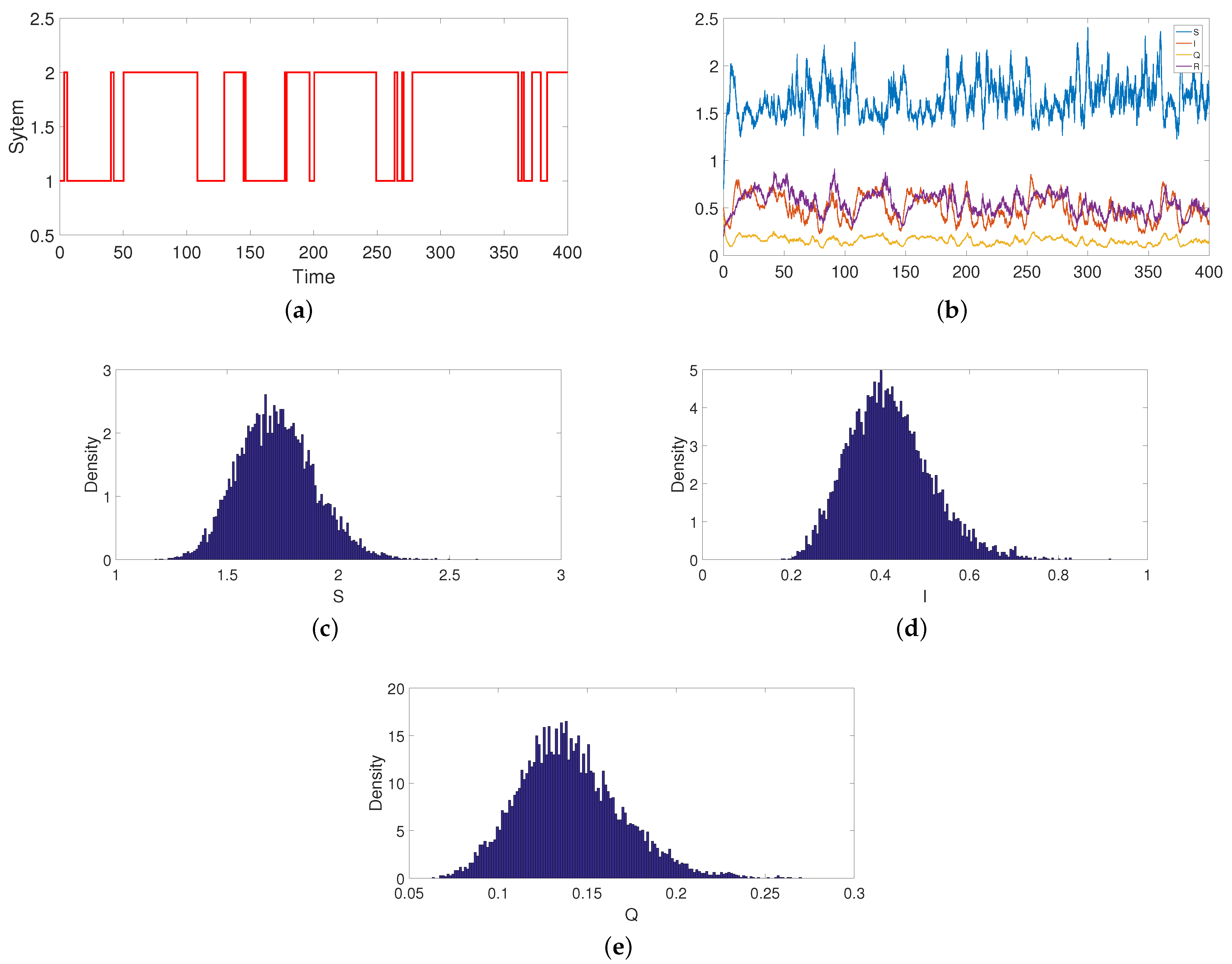
6. Numerical Simulations

In this section, one gives two examples to support the theoretical prediction.

Example 1.

In model (2), let $r\left(t\right)$ be a right-continuous Markov chain taking values $k=1,2$ and the generator Γ of the Markov chain is

$$\left(\begin{array}{cc}-0.06& 0.06\\ 0.04& -0.04\end{array}\right).$$

By solving the linear Equation (3), one can obtain the unique stationary distribution

$$\pi =({\pi }_1,{\pi }_2)=(0.4,0.6).$$

Choose the parameters values in model (2) as follows

$$\begin{array}{c}\hfill \mathsf{\Lambda }\left(1\right)=0.8,{\beta }_1\left(1\right)=0.6,{\beta }_2\left(1\right)=0.2,m\left(1\right)=1,N=1,\mu \left(1\right)=0.2,\alpha \left(1\right)=0.25,\end{array}$$

$$\begin{array}{c}\hfill \delta \left(1\right)=0.2,\gamma \left(1\right)=0.15,\epsilon \left(1\right)=0.2,{\sigma }_1\left(1\right)={\sigma }_2\left(1\right)={\sigma }_3\left(1\right)={\sigma }_4\left(1\right)=0.05.\end{array}$$

and

$$\begin{array}{c}\hfill \mathsf{\Lambda }\left(2\right)=1,{\beta }_1\left(2\right)=0.7,{\beta }_2\left(2\right)=0.1,m\left(1\right)=1,N=1,\mu \left(2\right)=0.3,\alpha \left(2\right)=0.3,\end{array}$$

$$\begin{array}{c}\hfill \delta \left(2\right)=0.3,\gamma \left(2\right)=0.25,\epsilon \left(2\right)=0.3,{\sigma }_1\left(2\right)={\sigma }_2\left(2\right)={\sigma }_3\left(2\right)={\sigma }_4\left(2\right)=0.1.\end{array}$$

Note that ${\mathfrak{R}}_1\approx 1.828>1$ holds, that is to say, the condition of Theorem 2 holds. Therefore, the stochastic model (2) has an ergodic stationary distribution. That means that the stochastic SIQR model (2) with regime switching has a unique stationary distribution and it has the ergodic property (see Figure 1).

Example 2.

In model (2), let $r\left(t\right)$ be a right-continuous Markov chain taking values $k=1,2$ and the generator Γ of the Markov chain is

$$\left(\begin{array}{cc}-0.06& 0.06\\ 0.04& -0.04\end{array}\right).$$

By solving the linear Equation (3), one can obtain the unique stationary distribution

$$\pi =({\pi }_1,{\pi }_2)=(0.4,0.6).$$

Choose the parameters values in model (2) as follows

$$\begin{array}{c}\hfill \mathsf{\Lambda }\left(1\right)=0.8,{\beta }_1\left(1\right)=0.25,{\beta }_2\left(1\right)=0.15,m\left(1\right)=1,N=1,\mu \left(1\right)=0.25,\alpha \left(1\right)=0.3,\end{array}$$

$$\begin{array}{c}\hfill \delta \left(1\right)=0.3,\gamma \left(1\right)=0.2,\epsilon \left(1\right)=0.2,{\sigma }_1\left(1\right)={\sigma }_2\left(1\right)={\sigma }_3\left(1\right)={\sigma }_4\left(1\right)=0.15.\end{array}$$

and

$$\begin{array}{c}\hfill \mathsf{\Lambda }\left(2\right)=1,{\beta }_1\left(2\right)=0.3,{\beta }_2\left(2\right)=0.2,m\left(1\right)=1,N=1,\mu \left(2\right)=0.3,\alpha \left(2\right)=0.35,\end{array}$$

$$\begin{array}{c}\hfill \delta \left(2\right)=0.4,\gamma \left(2\right)=0.4,\epsilon \left(2\right)=0.4,{\sigma }_1\left(2\right)={\sigma }_2\left(2\right)={\sigma }_3\left(2\right)={\sigma }_4\left(2\right)=0.2.\end{array}$$

Note that ${\mathfrak{R}}_2\approx 0.916<1$ holds, the condition of Theorem 3 is satisfied. Therefore, one can obtain that the disease $I\left(t\right)$ will tend to zero exponentially with probability one (see Figure 2).

7. Conclusions and Discussion

In this paper, A SIQR epidemic model with media coverage and regime switching is proposed. Firstly, the existence of the unique positive solution of the proposed system is studied. Secondly, some sufficient conditions for the existence of a stationary distribution by constructing a suitable random Lyapunov function are discussed. Meanwhile, the conditions for extinction are also obtained. Finally, some numerical simulation examples are carried out to demonstrate the effectiveness of theoretical results. With the development of network science, the epidemic model in networks has become a hot topic. In the future, some epidemic models with media coverage in the network can be considered [27,28].

The following abbreviations are used in this manuscript:

References

1. Ariful Kabir, K.M.; Kugaa, K.; Tanimotoc, J. Analysis of SIR epidemic model with information spreading of awareness. Chaos Solitons Fractals 2019, 119, 118–125. [Google Scholar] [CrossRef]
2. Chen, F. A susceptible-infected epidemic model with voluntary vaccinations. J. Math. Biol. 2006, 53, 253–272. [Google Scholar] [CrossRef] [PubMed]
3. Cao, X.; Jin, Z. Epidemic threshold and ergodicity of an SIS model in switched networks. J. Math. Anal. Appl. 2019, 479, 1182–1194. [Google Scholar] [CrossRef]
4. Guo, X.; Luo, J. Stationary distribution and extinction of SIR model with nonlinear incidence under Markovian switching. Phys. A Stat. Mech. Its Appl. 2018, 505, 471–481. [Google Scholar] [CrossRef]
5. Li, J.; Ma, Z. Qualitative analysis of SIS epidemic model with vaccination and varying total population size. Math. Comput. Model. 2002, 35, 1235–1243. [Google Scholar] [CrossRef]
6. Li, G.; Xu, X.; Zhang, M.; Liu, Q. Densely connected network for impulse noise removal. Pattern Anal. Appl. 2020, 23, 1263–1275. [Google Scholar] [CrossRef]
7. Meng, X.; Chen, L.; Wu, B. A delay SIR epidemic model with pulse vaccination and incubation times. Nonlinear Anal. Real World Appl. 2010, 11, 88–98. [Google Scholar] [CrossRef]
8. Shim, E.; Feng, Z.; Martcheva, M.; Chavez, C. An age-structured epidemic model of rotavirus with vaccination. J. Math. Biol. 2006, 53, 719–746. [Google Scholar] [CrossRef]
9. Xu, P.; Wu, S.; Huang, J. Ergodicity of stochastic damped higher-order KdV equation driven by white noise. Appl. Math. Lett. 2020, 110, 106575. [Google Scholar] [CrossRef]
10. Zhang, Y.; Fan, K.; Gao, S.; Liu, Y.; Chen, S. Ergodic stationary distribution of a stochastic SIRS epidemic model incorporating media coverage and saturated incidence rate. Phys. A Stat. Mech. Its Appl. 2019, 514, 671–685. [Google Scholar] [CrossRef]
11. Zhao, Y.; Jiang, D. The threshold of a stochastic SIS epidemic model with vaccination. Appl. Math. Comput. 2014, 243, 718–727. [Google Scholar] [CrossRef]
12. Cui, J.; Tao, X.; Zhu, H. An SIS infection model incorporating media coverage. Rocky Mt. J. Math. 2008, 38, 1323–1334. [Google Scholar] [CrossRef]
13. Ma, M.; Liu, S.; Li, J. Does media coverage influence the spread of drug addiction? Commun. Nonlinear Sci. Numer. Simul. 2017, 50, 169–179. [Google Scholar] [CrossRef]
14. Misra, A.; Sharma, A.; Shukla, J. Modeling and analysis of effects of awraencess programs by media on the spread of infectious diaeases. Math. Comput. Model. 2011, 53, 1221–1228. [Google Scholar] [CrossRef]
15. Zhang, T.; Meng, X. Stability analysis of a chemostat model with maintenance energy. Appl. Math. Lett. 2017, 68, 1–7. [Google Scholar] [CrossRef]
16. Liu, M.; He, X.; Yu, J. Dynamics of a stochastic regime-switching predator-prey model with harvesting and distributed delays. Nonlinear Anal. Hybrid Syst. 2018, 28, 87–104. [Google Scholar] [CrossRef]
17. Liu, Q.; Jiang, D.; Shi, N. Threshold behavior in a stochastic SIQR epidemic model with standard and regime switching. Appl. Math. Comput. 2018, 316, 310–325. [Google Scholar]
18. Lv, X.; Wang, L.; Meng, X. Global analysis of a new nonlinear stochastic differential competition system with impulsive effect. Adv. Differ. Equ. 2017, 2017, 296. [Google Scholar] [CrossRef] [Green Version]
19. Qi, H.; Zhang, S.; Meng, X.; Dong, H. Periodic solution and ergodic stationary distribution of two stochastic SIQS epidemic systems. Phys. A Stat. Mech. Its Appl. 2018, 508, 223–241. [Google Scholar] [CrossRef]
20. Yu, X.; Sun, Y.; Zhang, T. Persistence and ergodicity of a stochastic single species model with Allee effect under regime switching. Commun. Nonlinear Sci. Numer. Simul. 2018, 59, 359–374. [Google Scholar] [CrossRef]
21. Can, C.; Zhang, W. On observability and detectability of continuous-time stochastic Markov jump systems. J. Syst. Sci. Complex. 2015, 28, 830–847. [Google Scholar]
22. Khasminskii, R. Stochastic Stability of Differential Equation; Springer: Berlin, Germany, 2011. [Google Scholar]
23. Ma, H.; Jia, Y. Stability analysis for stochastics differential equations with infinite Markovian switchings. J. Math. Anal. Appl. 2016, 435, 593–605. [Google Scholar] [CrossRef]
24. Lipster, R. A strong law of large numbers for local martingales. Stochastics 1980, 3, 217–228. [Google Scholar]
25. Mao, X. Stationary distribution of stochastic population systems. Syst. Control Lett. 2011, 60, 398–405. [Google Scholar] [CrossRef] [Green Version]
26. Mao, X.; Marion, G.; Renshaw, E. Environmental brownian noise suppresses explosions in population dynamics. Stoch. Process. Appl. 2002, 97, 95–110. [Google Scholar] [CrossRef]
27. Kabir, K.A.; Tanimoto, J. Analysis of epidemic outbreaks in two-layer networks with different structures for information spreading and disease diffusion. Commun. Nonlinear Sci. Numer. Simul. 2019, 72, 565–574. [Google Scholar] [CrossRef]
28. Kabir, K.A.; Tanimoto, J. Vaccination strategies in a two-layer SIR/V–UA epidemic model with costly information and buzz effect. Commun. Nonlinear Sci. Numer. Simul. 2019, 76, 92–108. [Google Scholar] [CrossRef]
Figure 1. (a) is Markov chain, (b) is a stationary distribution of the stochastic model (2), (c) is the probability function of S ( t ) , (d) is the probability function of I ( t ) , (e) the probability function of Q ( t ) . The initial value is ( S ( 0 ) , I ( 0 ) , Q ( 0 ) , R ( 0 ) ) = ( 0.7 , 0.5 , 0.4 , 0.2 ) .
Symmetry 13 01122 g001
Figure 2. (a) is Markov chain, (b) is a stationary distribution of the stochastic model (2), (c) is the probability function of S ( t ) , (d) is the probability function of I ( t ) , (e) the probability function of Q ( t ) . The initial value is ( S ( 0 ) , I ( 0 ) , Q ( 0 ) , R ( 0 ) ) = ( 0.7 , 0.5 , 0.4 , 0.2 ) .
Symmetry 13 01122 g002
Publisher’s Note: MDPI stays neutral with regard to jurisdictional claims in published maps and institutional affiliations.