Article

Estimation and Prediction for Nadarajah-Haghighi Distribution under Progressive Type-II Censoring

Department of Mathematics, Beijing Jiaotong University, Beijing 100044, China
*
Author to whom correspondence should be addressed.
Symmetry 2021, 13(6), 999; https://doi.org/10.3390/sym13060999
Submission received: 9 May 2021 / Revised: 27 May 2021 / Accepted: 31 May 2021 / Published: 3 June 2021
(This article belongs to the Special Issue Probability, Statistics and Applied Mathematics)

Abstract

:
The paper discusses the estimation and prediction problems for the Nadarajah-Haghighi distribution using progressive type-II censored samples. For the unknown parameters, we first calculate the maximum likelihood estimates through the Expectation–Maximization algorithm. In order to choose the best Bayesian estimator, a loss function must be specified. When the loss is essentially symmetric, it is reasonable to use the square error loss function. However, for some estimation problems, the actual loss is often asymmetric. Therefore, we also need to choose an asymmetric loss function. Under the balanced squared error and symmetric squared error loss functions, the Tierney and Kadane method is used for calculating different kinds of approximate Bayesian estimates. The Metropolis-Hasting algorithm is also provided here. In addition, we construct a variety of interval estimations of the unknown parameters including asymptotic intervals, bootstrap intervals, and highest posterior density intervals using the sample derived from the Metropolis-Hasting algorithm. Furthermore, we compute the point predictions and predictive intervals for a future sample when facing the one-sample and two-sample situations. At last, we compare and appraise the performance of the provided techniques by carrying out a simulation study and analyzing a real rainfall data set.

1. Introduction

Nowadays, censoring has aroused great concern in the aspects of various reliability studies and life tests. There are already certain kinds of censoring schemes introduced in many references, among which type-I and type-II censoring are likely to be the two most famous types. Plenty of literature has discussed them, such as [1,2]. A life test in type-I censoring ends at a prespecified time, so the number of observations is random. By contrast, a life test in type-II censoring is not finished until a prefixed number of failures occur.
However, there are some constraints in type-I and type-II censoring. The units cannot be withdrawn when an experiment is in progress, for example. In this case, a kind of more flexible and more general censoring scheme named progressive type-II censoring scheme was put forward in order to improve this disadvantage. That is, it allows the removal of units in between. This scheme is introduced as follows. We assume that the number of n units are put in a life test. R 1 of the n 1 surviving units are withdrawn at random from the experiment as the first failure takes place. Likewise, after the second failure, R 2 out of the n R 1 2 remaining surviving units are randomly removed again. This experiment continues until m failures happen. The remaining units of size R m are withdrawn from the test at this moment, where R m = n m i = 1 m 1 R i . Then, R = ( R 1 , R 2 , , R m ) is named the progressive type-II censoring scheme, which should be prefixed before the experiment. Many statistical inferences and studies have been done involved with progressive censoring by several researchers like [3,4,5,6].
An extension of the exponential distribution was suggested by [7] by introducing a shape parameter. Its corresponding probability density function (PDF) is defined by
f ( x ; α , λ ) = α λ ( 1 + λ x ) α 1 exp { 1 ( 1 + λ x ) α } , x > 0 ; α > 0 , λ > 0 ,
and cumulative distribution function (CDF) is expressed as
F ( x ; α , λ ) = 1 exp { 1 ( 1 + λ x ) α } , x > 0 ; α > 0 , λ > 0 ,
where the shape and scale parameters are respectively α and λ . Both of them are positive. We denote this distribution by NH( α , λ ). In addition, the NH distribution in some other literature is also named the extended exponential distribution, such as [8,9].
Ref. [7] made a discovery that even though some data sets contained the value zero, an NH distribution still could provide suitable fits to them. In addition, the trend of hazard rate function is dependent on α in this distribution. For instance, the hazard rate function tends to increase (decrease) when α > 1 ( α < 1 ) , respectively. However, the hazard rate function turns into a constant as α is given the value of 1. At this time, (1) becomes the one-parameter exponential distribution as well.
Some literature can be found with regard to the statistical inferences for the NH distribution. As for the estimation of the unknown parameters, based on progressive type-II censored samples with binomial removals, Ref. [10] has discussed the maximum likelihood and Bayes estimations. Then, Ref. [11] researched progressive type-II censored data. They calculated the maximum likelihood estimates (MLEs) through the method of Newton–Raphson, and Bayes estimates through the Markov Chain Monte Carlo method. Interval estimations were made like asymptotic confidence intervals (CIs) and the highest posterior density (HPD) intervals as well. Several references also laid emphasis on the problems of order statistics of an NH distribution, such as [8,9]. They both worked on recurrence formulas of the moments for order statistics. However, the former dealt with the situation in progressive type-II right censoring while the latter focused on the complete samples. Additionally, for the unknown parameters, Ref. [12] discussed MLEs, and Bayesian estimates by the Lindley approximation. The point and interval predictions for future records were also made by making use of non-Bayesian and Bayesian predictions. In addition, based on the progressively first-failure censored NH distribution, Ref. [13] studied the MLEs and Bayes estimates for the two unknown parameters and lifetime parameters of survival and hazard rate functions. They also suggested an optimal censoring scheme through different optimality criteria.
In the article, using progressive type-II censored samples, we discuss the estimation and prediction problems for the NH distribution by diverse kinds of methods. In addition, we compare their performance through the simulation study and a real rainfall data set.
In Section 2, for the unknown parameters, we utilize the Expectation–Maximization (EM) algorithm for calculating the MLEs. Then, on the basis of the Fisher information matrix, we set up the asymptotic intervals. Furthermore, here bootstrap intervals are introduced as well. In Section 3, under two types of loss functions, Bayesian estimators of unknown parameters are calculated through both the Metropolis-Hasting (MH) method and Tierney and Kadane (TK) algorithm. Then, using the sample generated by the MH algorithm, we get the HPD credible intervals as well. In Section 4, Bayesian predictive intervals and the point prediction of a future sample are discussed. Additionally, we compare and appraise the performance of the provided techniques by carrying out a simulation study and analyzing a real data set in Section 5.

2. Maximum Likelihood Estimation

We assume that the number of n units are placed in a life test. They are independent and identically follow the NH distribution defined in (1). Under a progressive type-II censoring scheme R = ( R 1 , R 2 , , R m ) , let us denote a set of censored samples of size m by X = ( X 1 : m : n , X 2 : m : n , , X m : m : n ) from the NH distribution. In light of [3], the likelihood function related to α and λ is written as
l ( α , λ | x ̲ ) = κ i = 1 m f ( x i ; α , λ ) [ 1 F ( x i ; α , λ ) ] R i = κ ( α λ ) m i = 1 m ( 1 + λ x i ) α 1 exp { 1 ( 1 + λ x i ) α } exp { 1 ( 1 + λ x i ) α } R i ,
where κ = n ( n 1 R 1 ) ( n m + 1 i = 1 m 1 R i ) , and x ̲ = ( x 1 , x 2 , , x m ) stands for the corresponding observed value of X. Ignoring the constant, we compute the log-likelihood function by
L ( α , λ | x ̲ ) = ln l ( α , λ | x ̲ ) = m ln α λ + i = 1 m [ 1 ( 1 + λ x i ) ] α ( 1 + R i ) + ( α 1 ) i = 1 m ln ( 1 + λ x i ) .
As usual, to acquire the MLEs of α and λ , we are supposed to solve the corresponding likelihood equations as
L α = m α i = 1 m ( 1 + R i ) ( 1 + λ x i ) α ln ( 1 + λ x i ) + i = 1 m ln ( 1 + λ x i ) = 0 ,
L λ = m λ α i = 1 m ( 1 + R i ) x i ( 1 + λ x i ) α 1 + i = 1 m x i 1 + λ x i = 0 .
However, it is infeasible to solve the above equations analytically in closed form. Therefore, some numerical techniques like the EM algorithm are suggested for calculating the desired MLEs. As a solution to lost or partial data situations, Ref. [14] introduced the EM algorithm at first.
We are aware that the progressive type-II censored data are not complete, so they can be treated as a set of incomplete data. Now we assume that Z = ( Z 1 , Z 2 , , Z m ) represents censored data and X = ( X 1 : m : n , X 2 : m : n , , X m : m : n ) represents observed data. It is worth noting that for i = 1 , 2 , , m , every Z i is a set of 1 × R i vectors of ( Z i 1 , Z i 2 , , Z i R i ) . Consequently, observed data X combine censored data Z to form the complete data set as V = ( X , Z ) . We disregard the additive constant and then obtain the corresponding log-likelihood function L c ( V ; α , λ ) for V as
L c ( V ; α , λ ) = n ln α λ + ( α 1 ) i = 1 m ln ( 1 + λ x i ) + i = 1 m ( 1 ( 1 + λ x i ) α ) + ( α 1 ) i = 1 m k = 1 R i ln ( 1 + λ z i k ) + i = 1 m k = 1 R i ( 1 ( 1 + λ z i k ) α ) ,
where z i k denotes a censored value of Z i R i for k = 1 , , R i and i = 1 , , m .
The EM algorithm is composed of two parts named E-step and M-step. To begin with, the E-step is involved with calculation related to the corresponding pseudo-log-likelihood function as
L s ( α , λ ) = n ln α λ + ( α 1 ) i = 1 m ln ( 1 + λ x i ) + i = 1 m ( 1 ( 1 + λ x i ) α ) + ( α 1 ) i = 1 m i = 1 R i E ( ln ( 1 + λ z i k ) | z i k > x i ) + i = 1 m i = 1 R i E ( ( 1 ( 1 + λ z i k ) α ) | z i k > x i ) ,
where
E ( ln ( 1 + λ z i k ) | z i k > x i ) = 1 1 F ( x i ; α , λ ) x i + e 1 ( 1 + λ t ) α ln ( 1 + λ t ) ( 1 + λ t ) α 1 d t = 1 α 1 F ( x i ; α , λ ) 0 e 1 ( 1 + λ x i ) α ln ( 1 ln y ) d y = E 1 ( x i , α , λ ) , say
E ( 1 ( 1 + λ z i k ) α | z i k > x i ) = α λ 1 F ( x i ; α , λ ) x i + [ 1 ( 1 + λ t ) α ] ( 1 + λ t ) α 1 e 1 ( 1 + λ t ) α d t = 1 1 F ( x i ; α , λ ) 0 e 1 ( 1 + λ x i ) α ( ln y ) d y = ( 1 + λ x i ) α = E 2 ( x i , α , λ ) , say .
As for the M-step, the maximum value of (8) depends on the values of α and λ . We assume that the estimate of ( α , λ ) is referred to as ( α ( j ) , λ ( j ) ) in the jth iteration. Thus, we can figure out ( α ( j + 1 ) , λ ( j + 1 ) ) through maximizing the function
L s ( α , λ ) = n ln α λ + ( α 1 ) i = 1 m ln ( 1 + λ x i ) + ( α 1 ) i = 1 m R i E 1 ( x i , α ( j ) , λ ( j ) ) + i = 1 m ( 1 ( 1 + λ x i ) α ) + i = 1 m R i E 2 ( x i , α ( j ) , λ ( j ) ) .
As the values of α ( j ) and λ ( j ) are known, at first, λ ( j + 1 ) is calculated through solving the equation
L s λ = n λ ( j + 1 ) α ( j ) i = 1 m x i ( 1 + λ ( j + 1 ) x i ) α ( j ) 1 + ( α ( j ) 1 ) i = 1 m x i 1 + λ ( j + 1 ) x i = 0 .
Once λ ( j + 1 ) is obtained, we can also solve α ( j + 1 ) by the following equation
L s α = n α ( j + 1 ) + i = 1 m ln ( 1 + λ ( j + 1 ) x i ) i = 1 m ( 1 + λ ( j + 1 ) x i ) α ( j + 1 ) ln ( 1 + λ ( j + 1 ) x i ) + i = 1 m R i E 1 ( x i , α ( j ) , λ ( j + 1 ) ) = 0 .
Then, in the next iteration, we treat ( α ( j + 1 ) , λ ( j + 1 ) ) as the updated numeric value for ( α , λ ) . Like this, we proceed with the above two steps repeatedly before α and λ finally converge to their MLEs. According to [15], the log-likelihood function is ensured to increase with each iteration. As a result, the EM algorithm almost always manages to make the likelihood function attain its local maximum value despite beginning with a random value of the parameter domain. When, in Section 5, using the EM algorithm for MLEs under progressive type-II censoring, we take the MLEs derived from complete samples as initial values.

2.1. Fisher Information Matrix

Let θ denote the unknown parameter ( α , λ ) . We assume that V represents the complete data and X represents the observed data. Then, let us denote the observed, missing, and complete information by I X ( θ ) , I V | X ( θ ) , and I V ( θ ) , respectively. Based on the idea of [16], we can obtain
I X ( θ ) = I V ( θ ) I V | X ( θ ) ,
where
I V ( θ ) = E 2 L c ( V ; θ ) θ 2 = a 11 ( α , λ ) a 12 ( α , λ ) a 21 ( α , λ ) a 22 ( α , λ ) ,
and
I V | X j ( θ ) = E Z j | X j : m : n 2 ln f Z j ( z j | x j , θ ) θ 2 = b 11 ( x j ; α , λ ) b 12 ( x j ; α , λ ) b 21 ( x j ; α , λ ) b 22 ( x j ; α , λ ) .
We note that these are two 2 × 2 matrices. Moreover, I V | X j ( θ ) stands for the Fisher information matrix of one single observation which is censored as the jth failure occurs. Subsequently, we first calculate the elements of I V ( θ ) as follows.
a 11 ( α , λ ) = n α 2 + 1 α 2 0 + [ ln ( 1 + u ) ] 2 ( 1 + u ) e u d u , a 22 ( α , λ ) = n λ 2 + α 1 λ 2 0 + [ 1 + α ( 1 + u ) ] [ 1 ( 1 + u ) 1 α ] 2 e u d u , a 12 ( α , λ ) = a 21 ( α , λ ) = 1 λ 0 + [ 1 ( 1 + u ) 1 α ] [ ( 1 + u ) ln ( 1 + u ) + u ] e u d u .
From (16), we also have
b 11 ( x j ; α , λ ) = 1 α 2 + 1 [ 1 F ( x j ; α , λ ) ] α 2 ( 1 + λ x j ) α 1 + ( 1 + t ) [ ln ( 1 + t ) ] 2 e t d t + ( 1 + λ x j ) α [ ln ( 1 + λ x j ) ] 2 , b 22 ( x j ; α , λ ) = 1 λ 2 + α 1 [ 1 F ( x j ; α , λ ) ] λ 2 ( 1 + λ x j ) α 1 + [ 1 + α ( 1 + t ) ] [ 1 ( 1 + t ) 1 α ] 2 e t d t + α ( α 1 ) ( 1 + λ x j ) α 2 x j 2 , b 12 ( x j ; α , λ ) = b 21 ( x j ; α , λ ) = x j ( 1 + λ x j ) α 1 [ α ln ( 1 + λ x j ) + 1 ] + 1 λ [ 1 F ( x j ; α , λ ) ] ( 1 + λ x j ) α 1 + [ ( 1 + t ) ln ( 1 + t ) + t ] [ 1 ( t + 1 ) 1 α ] e t d t .
Then, we can calculate the total missing information matrix by the following expression
I V | X ( θ ) = j = 1 m R j I V | X j ( θ ) .
Based on the two matrices above, we easily compute the observed information matrix from (14) and its inverse matrix as well. The MLE θ ^ = ( α ^ , λ ^ ) has asymptotic normality, so we can write it as θ ^ N ( θ , I X 1 ( θ ^ ) ) . As a consequence, the 100 ( 1 p ) % asymptotic CIs are derived by
α ^ z p 2 V a r ( α ^ ) , α ^ + z p 2 V a r ( α ^ ) and λ ^ z p 2 V a r ( λ ^ ) , λ ^ + z p 2 V a r ( λ ^ ) ,
where 0 < p < 1 and z p 2 is a numerical number of the upper p 2 th percentile of the standard normal variate. Here, two elements of the main diagonal of I X 1 ( θ ^ ) are V a r ( α ^ ) and V a r ( λ ^ ) .

2.2. Bootstrap Confidence Intervals

As is known to us, the asymptotic CIs perform poorly in a sample with a small size. The bootstrap methods are more likely to provide more approximate confidence intervals. As a result, we introduce two CIs using the bootstrap methods. One is the percentile bootstrap (Boot-p) method which was put forward by [17]. According to [18], another is called the bootstrap-t (Boot-t) method. The Boot-p method and the Boot-t method are presented in Algorithms 1 and 2, respectively.
Algorithm 1 Boot-p method
Require: The number of simulation times N; the censoring scheme R; the confidence level 100 ( 1 p ) % ; the progressive type-II censored sample X
Ensure: The 100 ( 1 p ) % boot-p CI for φ , φ ^ B o o t p p 2 , φ ^ B o o t p 1 p 2 , where φ can be α and λ ;
1: Compute the MLE ( α ^ , λ ^ ) from X;
2: for v = 1 to N do
3:  Derive a bootstrap sample from the NH distribution by using ( α ^ , λ ^ ) under R;
4:  Calculate the MLE ( α ^ v * , λ ^ v * ) based on the bootstrap sample;
5: end for
6: Sort φ ^ v * , v = 1 , 2 , , N , ascendingly as φ ^ ( 1 ) * , φ ^ ( 2 ) * , , φ ^ ( N ) * ;
7: Compute φ ^ B o o t p p 2 = φ ^ ( [ p 2 N ] ) * and φ ^ B o o t p 1 p 2 = φ ^ ( [ ( 1 p 2 ) N ] ) * , where [ p 2 N ] is the largest integer that does not exceed p 2 N .
8: return φ ^ B o o t p p 2 , φ ^ B o o t p 1 p 2 ;
Algorithm 2 Boot-t method
Require: The number of simulation times N; the censoring scheme R; the confidence level 100 ( 1 p ) % ; the progressive type-II censored sample X
Ensure: The 100 ( 1 p ) % boot-t CI for φ , φ ^ B o o t t p 2 , φ ^ B o o t t 1 p 2 , where φ can be α and λ ;
1: Compute the MLE ( α ^ , λ ^ ) from X;
2: for v = 1 to N do
3:  Derive a bootstrap sample from the NH distribution by using ( α ^ , λ ^ ) under R;
4:  Calculate the MLE ( α ^ v * , λ ^ v * ) based on the bootstrap sample;
5:  Compute the statistic T v * = φ ^ v * φ ^ V a r ( φ ^ v * ) ;
6: end for
7: Sort T 1 * , T 2 * , , T N * ascendingly as T ( 1 ) * , T ( 2 ) * , , T ( N ) * ;
8: Pick T ( [ p 2 N ] ) * , T ( [ ( 1 p 2 ) N ] ) * , and their corresponding MLEs φ ^ L * , φ ^ R * ;
9: Compute φ ^ B o o t t ( p 2 ) = φ ^ + V a r ( φ ^ L * ) T ( [ p 2 N ] ) * and φ ^ B o o t t ( 1 p 2 ) = φ ^ + V a r ( φ ^ R * ) T ( [ ( 1 p 2 ) N ] ) * ;
10: return φ ^ B o o t t p 2 , φ ^ B o o t t 1 p 2 ;

3. Bayesian Estimation

In order to choose the best Bayesian estimator, a loss function must be specified and used to represent the penalty associated with each possible estimator. Researchers usually use the symmetric squared error loss function. There is no doubt that it is reasonable to use the squared error loss function when the loss is essentially symmetric. However, for some estimation problems, the actual loss is often asymmetric. Therefore, we also need to choose an asymmetric loss function.
We consider Bayesian estimators under symmetric and asymmetric loss functions. We suppose that δ is a Bayesian estimate for θ . Firstly, the symmetric squared error loss (SEL) function is written as
L S ( θ , δ ) = ( δ θ ) 2 .
Hence, under L S ( θ , δ ) , the Bayesian estimate for θ is expressed by
δ S = E ( θ | x ̲ ) .
In light of [19], the balanced squared error loss (BSEL) function has the following form:
L B ( θ , δ ) = ( 1 ϵ ) ( δ θ ) 2 + ϵ ( δ δ 0 ) 2 ,
where 0 ϵ 1 , and δ 0 is a known estimate of θ . It is worth noting that when ϵ is given as the value of 0, the BESL function turns into the SEL function. Based on the BSEL function L B ( θ , δ ) , the Bayes estimator is calculated by
δ B = ϵ δ 0 + ( 1 ϵ ) E ( θ | x ̲ ) .
Let us denote a set of progressive type-II censored samples by X = ( X 1 : m : n , X 2 : m : n , , X m : m : n ) from the NH distribution. Suppose that two independent parameters α and λ follow the gamma prior distributions as
α G a m m a ( a , b ) and λ G a m m a ( c , d ) , α , λ > 0 , a , b , c , d > 0 .
Here, the prior information is shown by selecting the numerical numbers for four hyperparameters a , b , c , and d. Hence, the joint prior density is expressed by
ϕ ( α , λ ) α a 1 e b α λ c 1 e d λ .
Consequently, the joint posterior density is then obtained by
ϕ ( α , λ | x ̲ ) = l ( α , λ | x ̲ ) ϕ ( α , λ ) 0 + 0 + ϕ ( α , λ ) l ( α , λ | x ̲ ) d α d λ = ϱ 1 α a + m 1 λ c + m 1 e b α d λ i = 1 m ( 1 + λ x i ) α 1 exp ( 1 + R i ) 1 ( 1 + λ x i ) α ,
where ϱ denotes a normalizing constant.
As we can see, it is impractical to deal with the joint posterior distribution analytically. The Bayesian estimators of some functions involved with α and λ also include the rates between two integrals. Therefore, as we calculate Bayesian estimators based on these two kinds of loss functions, two approximate methods are proposed to cope with the corresponding ratio of integrals in the next two subsections, respectively.

3.1. Tierney and Kadane Method

Based on the idea of [20], we take advantage of the TK method and then calculate approximate Bayes estimates. The posterior expectation for ξ ( α , λ ) can be expressed as
Ψ ( x ̲ ) = 0 + 0 + exp { Φ ( α , λ ) + L ( α , λ | x ̲ ) } ξ ( α , λ ) d α d λ 0 + 0 + exp { Φ ( α , λ ) + L ( α , λ | x ̲ ) } d α d λ = 0 + 0 + exp { n ψ ξ * } d α d λ 0 + 0 + exp { n ψ } d α d λ ,
where Φ ( α , λ ) = ln ϕ ( α , λ ) , and L ( α , λ | x ̲ ) represents the log-likelihood function (4). Moreover, ψ ( α , λ ) and ψ ξ * ( α , λ ) are defined as
ψ ( α , λ ) = Φ ( α , λ ) + L ( α , λ | x ̲ ) n and ψ ξ * ( α , λ ) = ψ ( α , λ ) + ln ξ ( α , λ ) n .
Suppose that ( α ^ ψ , λ ^ ψ ) and ( α ^ ψ * , λ ^ ψ * ) respectively maximize the functions ψ ( α , λ ) and ψ ξ * ( α , λ ) . Through the TK method, Ψ ( x ̲ ) is approximated as
Ψ ( x ̲ ) = Σ ξ * Σ exp n [ ψ ξ * ( α ^ ψ * , λ ^ ψ * ) ψ ( α ^ ψ , λ ^ ψ ) ] .
Here, the determinants of negative inverse Hessian for ψ ( α , λ ) and ψ ξ * ( α , λ ) are Σ and Σ ξ * , respectively. Note that Σ and ( α ^ ψ , λ ^ ψ ) in (27) do not depend on the function ξ ( α , λ ) while the other two expressions do rely on ξ ( α , λ ) . We observe that
ψ ( α , λ ) = 1 n ( a + m 1 ) ln α + ( c 1 + m ) ln λ + i = 1 m [ 1 ( 1 + λ x i ) α ] = + ( α 1 ) i = 1 m ln ( 1 + λ x i ) + i = 1 m R i [ 1 ( 1 + λ x i ) α ] ( b α + d λ ) .
Then, ( α ^ ψ , λ ^ ψ ) are solved by the system of equations:
ψ α = 1 n a + m 1 α b + i = 1 m ln ( 1 + λ x i ) i = 1 m ( 1 + R i ) ( 1 + λ x i ) α ln ( 1 + λ x i ) = 0 ,
ψ λ = 1 n c + m 1 λ d + ( α 1 ) i = 1 m x i 1 + λ x i α i = 1 m ( 1 + R i ) x i ( 1 + λ x i ) α 1 = 0 .
The relevant second partial derivatives can be also computed by
2 ψ α 2 = 1 n a + m 1 α 2 i = 1 m ( 1 + R i ) ( 1 + λ x i ) α [ ln ( 1 + λ x i ) ] 2 ,
2 ψ α λ = 2 ψ λ α = 1 n i = 1 m x i 1 + λ x i i = 1 m ( 1 + R i ) 1 + α ln ( 1 + λ x i ) x i ( 1 + λ x i ) α 1 ,
and
2 ψ λ 2 = 1 n c + m 1 λ 2 α ( α 1 ) i = 1 m ( 1 + R i ) x i 2 ( 1 + λ x i ) α 2 ( α 1 ) i = 1 m x i 2 ( 1 + λ x i ) 2 .
Next, we obtain Σ as
Σ = 2 ψ α 2 2 ψ λ 2 2 ψ α λ 2 ψ λ α 1 .
As for Σ ξ * , we first obtain ( α ^ ψ * , λ ^ ψ * ) from the following expressions:
ψ * α = ψ α + ξ α n ξ ( α , λ ) = 0 ,
ψ * λ = ψ λ + ξ λ n ξ ( α , λ ) = 0 .
Then, the corresponding second-order derivatives are obtained as
2 ψ * α 2 = 2 ψ α 2 + ξ α α ξ ( α , λ ) ( ξ α ) 2 n [ ξ ( α , λ ) ] 2 ,
2 ψ * λ 2 = 2 ψ λ 2 + ξ λ λ ξ ( α , λ ) ( ξ λ ) 2 n [ ξ ( α , λ ) ] 2 ,
2 ψ * λ α = 2 ψ * α λ = 2 ψ α λ + ξ α λ ξ ( α , λ ) ξ α ξ λ n [ ξ ( α , λ ) ] 2 .
Next, we obtain Σ ξ * as
Σ ξ * = 2 ψ * α 2 2 ψ * λ 2 2 ψ * α λ 2 ψ * λ α 1 .
For the reason that Σ ξ * and ψ ξ * ( α , λ ) in (27) depend on the function ξ ( α , λ ) , we respectively take ξ ( α , λ ) = α and ξ ( α , λ ) = λ when proceeding with the above computation steps. Therefore, the Bayes estimates through the TK method can be calculated as
α ˜ T K = Σ α * Σ exp n [ ψ α * ( α ^ ψ * , λ ^ ψ * ) ψ ( α ^ ψ , λ ^ ψ ) ] , λ ˜ T K = Σ λ * Σ exp n [ ψ λ * ( α ^ ψ * , λ ^ ψ * ) ψ ( α ^ ψ , λ ^ ψ ) ] .
In the same way, the corresponding Bayesian estimates are also calculated based on the BSEL function. Here, we do not go into details for the sake of brevity.

3.2. Metropolis-Hastings Algorithm

As we can see from the previous subsection, for the unknown parameters, the TK method is not able to make interval estimates. Thus, we introduce another method called the MH algorithm to obtain some approximate Bayesian point and interval estimations. The MH algorithm is a very general type of Markov Chain Monte Carlo technique. For the first time, Ref. [21] suggested this technique. Then, it was expanded based on the idea of [22]. From their studies, we are aware that no matter how complex the known target distribution is, the MH algorithm can still derive random samples from it.
A bivariate normal distribution is treated as the proposal distribution for α and λ . Using the posterior density, for unknown parameters, we can derive samples from it so as to calculate Bayesian point estimators and HPD interval estimations. We present the main steps of the MH algorithm in Algorithm 3.
For the sake of ensuring the convergence and reducing some effects brought by ( α 0 , λ 0 ) , we abandon the initial N 0 number and then compute estimates from the rest of the N N 0 samples. Therefore, using the SEL function, we can calculate the Bayesian estimates by
η ˜ M H = 1 N N 0 q = N 0 + 1 N η i ,
where η can be α and λ .
Likewise, we also calculate the corresponding Bayes estimates based on the BSEL function. In addition, the 100 ( 1 p ) % HPD credible intervals are set up as well according to [23]. We sort the rest of samples in ascending order to be η ( N 0 + 1 ) , η ( N 0 + 2 ) , , η ( N ) . Then, we can compute the 100 ( 1 p ) % Bayes interval estimate of η as
η ( q ) , η ( q + [ ( 1 p ) × ( N N 0 ) ] ) , q = N 0 + 1 , , N N 0 ( 1 p ) × ( N N 0 ) .
The shortest interval among (39) is taken as the 100 ( 1 p ) % HPD interval of η .
Algorithm 3 MH algorithm
Require: The joint posterior distribution ϕ ( α , λ | x ̲ ) ; the initial values ( α 0 , λ 0 ) ; the number of simulation times N; the variance–covariance matrix Σ M H .
Ensure: The N number of samples ( α q , λ q ) , q = 1 , 2 , , N ;
1: for  q = 1 to N do
2:  Generate ( α * , λ * ) from the bivariate normal N 2 ( ( α q 1 , λ q 1 ) , Σ M H ) ;
3:  Calculate γ = min { 1 , ϕ ( α * , λ * | x ̲ ) ϕ ( α q 1 , λ q 1 | x ̲ ) } ;
4:  Derive a figure β that follows a Uniform ( 0 , 1 ) distribution;
5:  if β γ then
6:    ( α q , λ q ) ( α * , λ * ) ;
7:  else
8:    ( α q , λ q ) ( α q 1 , λ q 1 ) ;
9:  end if
10: end for
11: return ( α q , λ q ) , q = 1 , 2 , , N ;

4. Bayesian Prediction

We consider estimates of future samples in terms of known information and compute corresponding predictive intervals as well. Using the predictive distribution, the Bayesian approach on the prediction of future samples is treated as a significant topic in statistics. Subsequently, in the light of [24], we make discussions about Bayesian prediction facing the one-sample and two-sample situations indicated.

4.1. One-Sample Prediction

Let us denote a set of m progressive type-II censored data by X = ( X 1 : m : n , X 2 : m : n , , X m : m : n ) . It is obtained from n samples which follow the NH distribution described in (1) based on a censoring scheme R = ( R 1 , R 2 , , R m ) . Suppose that Z i = ( Z i 1 , Z i 2 , , Z i R i ) stands for the ordered statistic of R i removed units as the ith failure is observed. Using the observed samples x ̲ , we focus on predicting the value of z = ( z i k , k = 1 , , R i ; i = 1 , m ) . As a consequence, we can get the conditional density of z as
f i k ( z | x ̲ , α , λ ) = k R i k [ 1 F ( z ) ] R i k [ F ( z ) F ( x i ) ] k 1 f ( z ) [ 1 F ( x i ) ] R i = k R i k j = 0 k 1 ( 1 ) k 1 j k 1 j [ 1 F ( z ) ] R i 1 j f ( z ) 1 F ( x i ) j R i , z > x i .
According to the conditional density, the survival function can be expressed by
S i k ( t | x ̲ , α , λ ) = P ( z > t | x ̲ , α , λ ) P ( z > x i | x ̲ , α , λ ) = t + f i k ( z | x ̲ , α , λ ) d z x i + f i k ( z | x ̲ , α , λ ) d z = j = 0 k 1 ( 1 ) k 1 j k 1 j [ 1 F ( y ) ] R i j [ 1 F ( t ) ] j R i R i j j = 0 k 1 ( 1 ) k 1 j k 1 j 1 R i j .
Therefore, based on a prior ϕ ( α , λ | x ̲ ) , the associated posterior predictive density is given by
g ( z | x ̲ ) = 0 + 0 + ϕ ( α , λ | x ̲ ) f i k ( z | x ̲ , α , λ ) d α d λ ,
and posterior survival function is also given by
S i k * ( z | x ̲ ) = 0 + 0 + ϕ ( α , λ | x ̲ ) S i k ( z | x ̲ , α , λ ) d α d λ .
Consequently, the two-sided 100 ( 1 p ) % symmetric predictive interval ( L o , U o ) of z is the solution to the following equations:
S i k * ( L o | x ̲ ) = 1 p 2 and S i k * ( U o | x ̲ ) = p 2 .
As for the point prediction of the kth future sample z of the R i surviving units, on the basis of the SEL function, it is predicted by
z ^ = x i + z g ( z | x ̲ ) d z = 0 + 0 + x i + z ϕ ( α , λ | x ̲ ) f i k ( z | x ̲ , α , λ ) d z d α d λ = 0 + 0 + ϕ ( α , λ | x ̲ ) G ( x i | α , λ ) d α d λ ,
where
G ( x i | α , λ ) = x i + z f i k ( z ) d z = k R i k j = 0 k 1 ( 1 ) k 1 j [ 1 F ( x i ) ] j R i k 1 j x i + u [ 1 F ( u ) ] R i j 1 f ( u ) d u .
In our model, we then obtain that
G ( x i | α , λ ) = k R i k j = 0 k 1 ( 1 ) k 1 j e ( j R i ) [ 1 ( λ x i + 1 ) ] α k 1 j ( λ x i + 1 ) α 1 + 1 + ( 1 + t ) 1 α λ e ( R i j ) t d t .
We note that we cannot evaluate the above expressions analytically. Thus, we adopt the MH algorithm to tackle this problem and then compute the point predictions. Assume that ( α q , λ q ) , q = 1 , 2 , , N denote the samples which are derived from the posterior distribution. Therefore, we can compute the point prediction for z as
z ^ = 1 N N 0 q = N 0 + 1 N G ( x i | α q , λ q ) .

4.2. Two-Sample Prediction

We generally consider the prediction in a two-sample situation as an extension of that in a one-sample situation. There are two samples in the two-sample prediction problem. One is named the informative sample, and another is referred to as the future sample. Suppose that W = ( W 1 , W 2 , , W M ) of size M stands for the ordered statistic of future observations, and it is independent of the informative sample X = ( X 1 : m : n , , X m : m : n ) . Thus, we focus on making predictions of observation of the jth failure of a future sample W generated identically from the target distribution. Therefore, we can calculate the predictive density of W j by
f j ( w j | α , λ ) = j M j k = 0 j 1 ( 1 ) j 1 k j 1 k [ 1 F ( w j ) ] M 1 k f ( w j ) ,
where w j denotes the value of W j . Then, the survival function can be computed as
S j ( u | α , λ ) = P ( w j > u ) .
Consequently, the posterior survival function is written by
S j ( w j | x ̲ ) = 0 + 0 + ϕ ( α , λ | x ̲ ) S j ( w j | x ̲ , α , λ ) d α d λ ,
where x ̲ = ( x 1 , x 2 , , x m ) . The two-sided 100 ( 1 p ) % symmetric predictive interval ( L t , U t ) of w j is the solution to the following expressions:
S ( L t | x ̲ ) = 1 p 2 and S ( U t | x ̲ ) = p 2 .
The posterior density is also obtained as
h ( w j | x ̲ ) = 0 + 0 + f j ( w j | α , λ ) ϕ ( α , λ | x ̲ ) d α d λ .
Then, we can compute the point prediction of jth order lifetime as
w j ^ = 0 + w j h ( w j | x ̲ ) d w j = 0 + 0 + 0 + ϕ ( α , λ | x ̲ ) w j f ( w j | α , λ ) d w j d α d λ = 0 + 0 + ϕ ( α , λ | x ̲ ) H ( α , λ ) d α d λ ,
where
H ( α , λ ) = 0 + w j f ( w j | α , λ ) d w j = j M j k = 0 j 1 ( 1 ) j 1 k j 1 k 0 + ( t + 1 ) 1 α 1 λ e ( M k ) t d t .
Using the MH algorithm as in the previous subsection, we can calculate the point prediction of a future sample W j as
w j ^ = 1 N N 0 q = N 0 + 1 N H ( α q , λ q ) .

5. Data Analysis and Simulation Study

For the purpose of demonstrating practical applications of provided techniques on estimation and prediction problems, in the next two subsections, we compare and appraise their performance by carrying out a simulation study and analyzing real data, respectively.

5.1. Data Analysis

We consider a set of real data on the total annual rainfall (unit: inches) during January from 1880 to 1916 researched by [12]. It is listed in Table 1 below.
With an aim to analyze real data, at first, we calculate the MLEs through the EM algorithm and then figure out the Akaike information criterion (AIC), Bayesian information criterion (BIC), and Kolmogorov–Smirnov (K–S) statistics for goodness-of-fit tests. For comparison, some other life distributions are also put on goodness-of-fit tests, such as Generalized Exponential, Chen, and Inverse Weibull distributions. Their PDFs are given as below, respectively.
(1)
The PDF of the Generalized Exponential distribution is
f 1 ( x ; α , λ ) = α λ e λ x ( 1 e λ x ) α 1 , x > 0 , α , λ > 0 .
(2)
The PDF of the Chen distribution is
f 2 ( x ; α , λ ) = α λ x λ 1 exp x λ + α ( 1 e x λ ) , x > 0 , α , λ > 0 .
(3)
The PDF of the Inverse Weibull distribution is
f 3 ( x ; α , λ ) = α λ x ( α + 1 ) exp { λ x α } , x > 0 , α , λ > 0 .
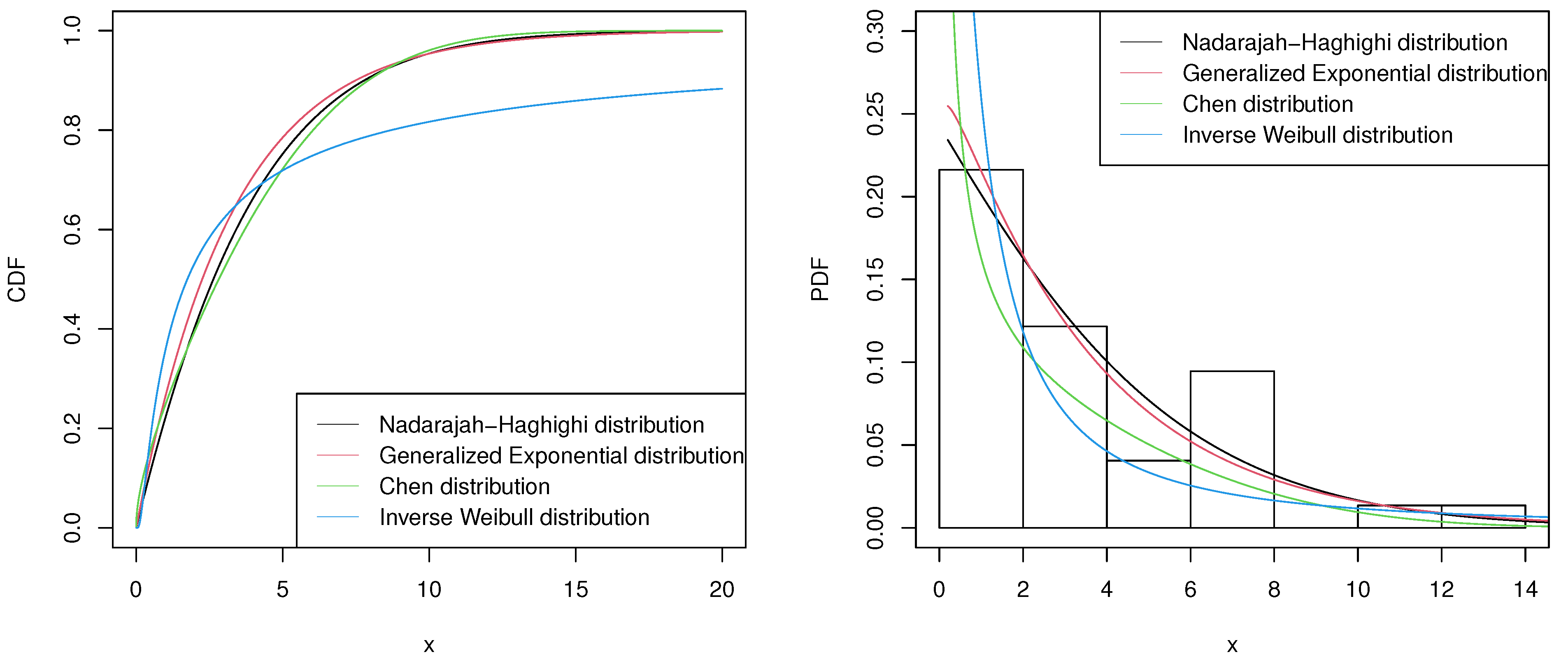
Table 2 presents all the test results of these distributions. As we all know, the smaller the numerical values of K–S, AIC, and BIC are, the bigger the log-likelihood function value is, and the better the model performs. Therefore, it can be seen from the table that the NH distribution provides a more suitable fit to this set of real data. For more fitting illustration, two plots made through the MLEs are provided in Figure 1. The first plot contains the fitted CDFs of the Nadarajah-Haghighi, Generalized Exponential, Chen, and Inverse Weibull distributions for the real data set. The second plot consists of the histogram of the real data and the fitted PDFs of these four distributions.
Next, we get two sets of censored data under two dissimilar progressive type-II censored schemes. They are r s 1 = ( 0 * 5 , 3 , 0 , 2 , 2 , 1 , 0 * 7 , 2 , 0 * 6 , 2 ) and r s 2 = ( 0 * 10 , 2 , 0 , 2 , 1 , 0 * 8 , 1 , 0 * 6 , 1 ) , respectively, where short notation 0 * 5 denotes 0 , 0 , 0 , 0 , 0 . The two corresponding sets of observed data are presented in Table 3 and Table 4.
Then, we obtain some statistical inferences for the two sets of data. For the unknown parameters, we calculate TK and MH estimations accompanied by their MLEs under different loss functions in Table 5. Then we tabulate some interval estimations of α and λ in Table 6 which include 90 % asymptotic CIs, 95 % bootstrap CIs, and 95 % HPD interval. Additionally, in Table 7, in the one-sample situation, we tabulate point predictions and the 95 % predictive intervals for the kth experimental unit which is censored at the ith failure. Furthermore, Table 8 includes the point prediction and also the 95% predictive intervals for the top five items of future observations of size 25 and 30 under the two-sample framework, respectively.

5.2. Simulation Study

We implement a simulation study for comparison of numerical results and then evaluate the proposed methods. Using different censoring schemes, we first derive progressive type-II censored samples that follow an NH ( α ˜ , λ ˜ ) distribution, where α ˜ = 1.4 and λ ˜ = 0.2 are true values we choose. Next, the EM algorithm can be applied so as to compute the MLEs. Afterwards, we give hyperparameters ( a , b , c , d ) the values as ( 0.5 , 1.7 , 0.5 , 5.6 ) . The Bayesian estimators under two different types of loss functions are calculated by the TK and MH methods. We take the mean-squared error (MSE) values into account for comparing these Bayes estimates with different methods. The MSEs of α and λ have the following forms
M S E α = 1 N q = 1 N ( α ^ q α ˜ ) 2 and M S E λ = 1 N q = 1 N ( λ ^ q λ ˜ ) 2 ,
where α ^ q and λ ^ q denote the estimates of α and λ at qth simulation time from different methods.
Different values of ϵ in the BSEL functions are considered as a kind of measure of its influence on Bayes estimates. In addition, all the ( n , m ) and censored schemes are shown in the tables, where m denotes the quantity of observed samples and n denotes the quantity of complete samples.
In Table 9, we tabulate average estimators and also the values of MSEs for α and λ under diverse censoring schemes. For each ( n , m ) with each censoring scheme, the first and the second rows show the average estimators of α and their MSEs. In addition, the average estimators of λ and their MSEs are shown in the third and fourth rows. This table demonstrates that the estimators computed through the MH algorithm have better performance than those obtained by the TK method. Additionally, Bayes estimates almost always play a more prominent role than the corresponding MLEs.
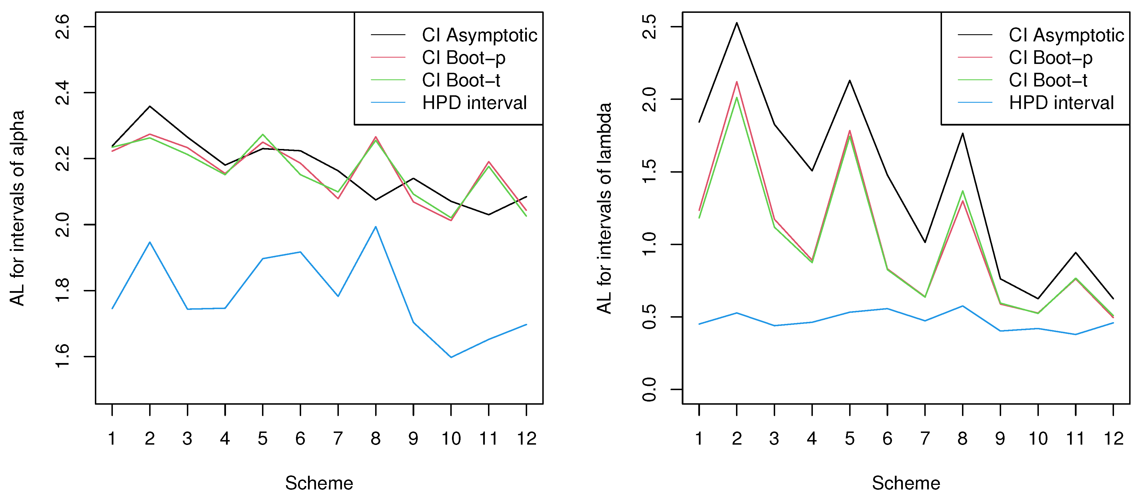
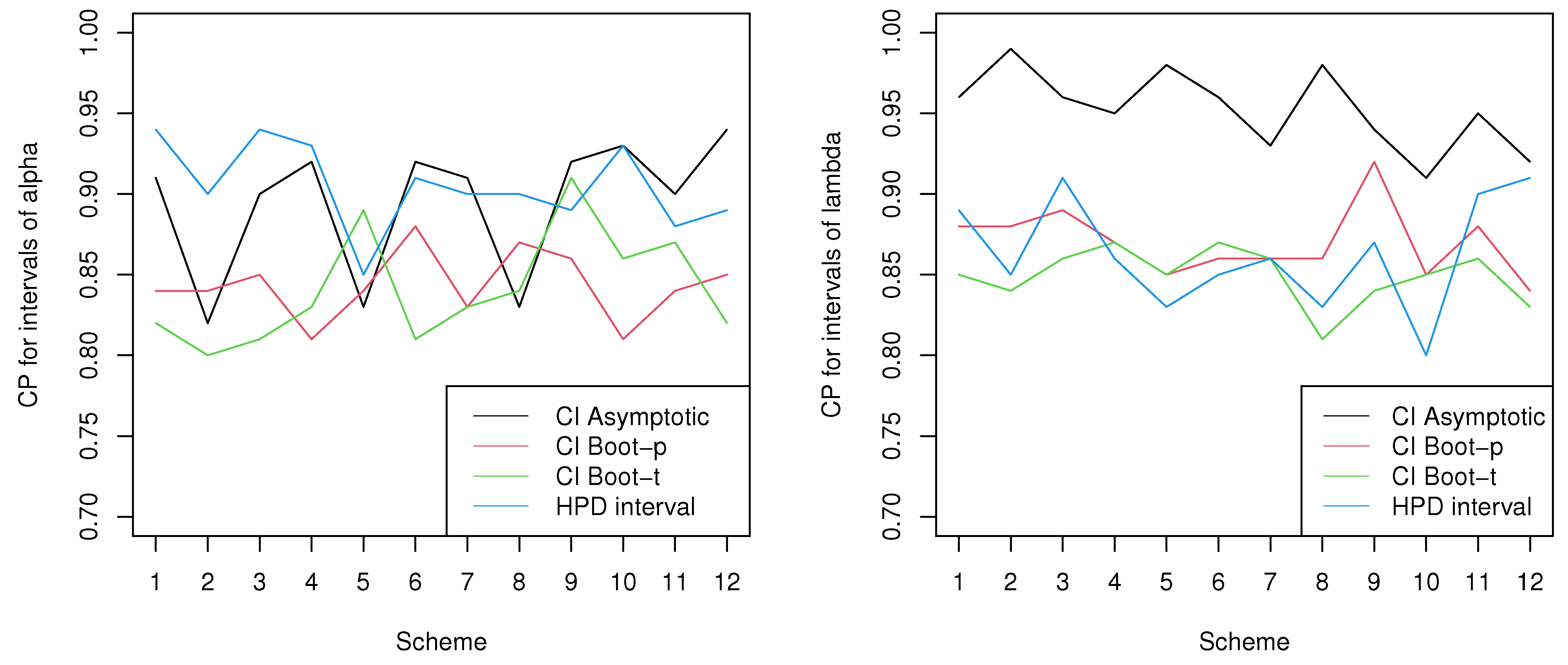
In Table 10, under pre-specified sample sizes and censoring schemes, we construct varieties of interval estimations for the unknown parameters along with their coverage probabilities (CPs) and average length (AL). In each ( n , m ) with each censoring scheme, the first and second rows respectively show the statistical inferences of α and λ . For more illustration, we also provide four plots in Figure 2 and Figure 3, where the numbers 1 to 12 on the x-axis denote all the schemes from top to bottom in the table. Figure 2 includes the AL for different intervals of α and λ under different schemes, respectively. In addition, under different schemes, the CPs for different intervals of α and λ are provided in Figure 3.
As we can see, the AL of the HPD intervals are the shortest, followed by the bootstrap intervals, and the asymptotic intervals are the longest. However, as for the CPs, the asymptotic intervals hold the highest, followed by the HPD intervals, while the CPs of bootstrap often lie below the nominal level. Therefore, considering both AL and CPs, we believe that the asymptotic and bootstrap intervals are inferior to the HPD intervals.
In Table 11, we compute point prediction and 95% predictive intervals for different censored observations using the MH algorithm. We can see from the predicted intervals that when we censor more than one unit at a time, the AL of the prediction intervals of the unit censored at the early stage is shorter than that at the late stage. However, when we censor just one unit many times, we find that the later the stage is, the smaller the AL of the interval prediction is. The AL of prediction intervals is inclined to shorten as the observed sample grows in number.
In Table 12, under the two-sample prediction frame, we tabulate the point predictions and 95 % predictive intervals of the first, the third, and the fifth future observations of total size 5. It is worth noting that the lengths for these interval predictions are prone to become longer with the increasing value of j. As a consequence, M = m is taken into consideration when the real data are under analysis.

6. Conclusions

This article provides the classical and Bayesian estimations for Nadarajah-Haghighi distribution using progressive type-II censored samples. As for the unknown parameters, we compute maximum likelihood estimates through an Expectation–Maximization algorithm. Under two different kinds of loss functions including the balanced squared error and squared error loss functions, we calculate varieties of approximate Bayes estimates using both the Metropolis-Hasting algorithm and the Tierney and Kadane method. In addition, we get estimation results of confidence intervals, which include the asymptotic intervals, and bootstrap intervals. Then, using the sample derived from the Metropolis-Hasting algorithm, we also obtain the highest posterior density intervals. Furthermore, the point and interval prediction for a future sample is considered in the one-sample and two-sample situations. In the end, we compare and appraise the performance of the provided techniques through a simulation study. For further explanation, one set of real rainfall data is also analyzed.
Overall, we can learn from the numerical studies that the proposed methods can work well. For instance, compared with maximum likelihood estimates and the Bayes estimates using the Tierney and Kadane method, the Bayes estimates using the Metropolis-Hasting algorithm are quite closer to the true values of unknown parameters. The MSEs are mostly less than 0.1 . In addition, in Table 7, we can see that the true values of censored samples are completely in the predictive intervals.
Additionally, the methods provided in this article can be extended to other life distributions.

Author Contributions

Investigation, M.W.; Supervision, W.G. All authors have read and agreed to the published version of the manuscript.

Funding

This research was supported by Project 202110004106 supported by Beijing Training Program of Innovation and Entrepreneurship for Undergraduates.

Data Availability Statement

The data presented in this study are openly available in reference [12].

Conflicts of Interest

The authors declare no conflict of interest.

References

  1. Balakrishnan, N.; Cohen, A.C. Order Statistics and Inference: Estimation Methods; Academic Press: Boston, MA, USA, 1991. [Google Scholar]
  2. Lawless, J.F. Statistical Models and Methods for Lifetime Data; Wiley: New York, NY, USA, 1982. [Google Scholar]
  3. Balakrishnan, N.; Aggarwala, R. Progressive Censoring: Theory, Methods, and Applications; Birkhäuser: Boston, MA, USA, 2000. [Google Scholar]
  4. Cohen, A.C. Truncated and Censored Samples: Theory and Applications; Marcel Dekker: New York, NY, USA, 1991. [Google Scholar]
  5. Rastogi, M.K.; Tripathi, Y.M.; Wu, S.-J. Estimating the parameters of a bathtub-shaped distribution under progressive type-II censoring. J. Appl. Stat. 2012, 39, 2389–2411. [Google Scholar] [CrossRef]
  6. Ren, J.; Gui, W. Inference and optimal censoring scheme for progressively type-ii censored competing risks model for generalized rayleigh distribution. Comput. Stat. 2020, 36, 479–513. [Google Scholar] [CrossRef]
  7. Nadarajah, S.; Haghighi, F. An extension of the exponential distribution. Statistics 2011, 45, 543–558. [Google Scholar] [CrossRef]
  8. Kumar, D.; Dey, S.; Nadarajah, S. Extended exponential distribution based on order statistics. Commun. Stat. Theory Methods 2017, 46, 9166–9184. [Google Scholar] [CrossRef]
  9. Kumar, D.; Malik, M.R.; Dey, S.; Shahbaz, M.Q. Recurrence relations for moments and estimation of parameters of extended exponential distribution based on progressive type-II right-censored order statistics. J. Stat. Theory Appl. 2019, 18, 171–181. [Google Scholar] [CrossRef] [Green Version]
  10. Singh, S.; Singh, U.; Kumar, M.; Vishwakarma, P. Classical and Bayesian inference for an extension of the exponential distribution under progressive type-II censored data with binomial removals. J. Stat. Appl. Probab. Lett. 2014, 1, 75–86. [Google Scholar] [CrossRef]
  11. Singh, U.; Singh, S.K.; Yadav, A.S. Bayesian estimation for extension of exponential distribution under progressive type-II censored data using Markov Chain Monte Carlo method. J. Stat. Appl. Probab. 2015, 4, 275–283. [Google Scholar]
  12. Selim, M.A. Estimation and prediction for Nadarajah-Haghighi distribution based on record values. Pak. J. Stat. 2018, 34, 77–90. [Google Scholar] [CrossRef]
  13. Ashour, S.K.; El-Sheikh, A.A.; Elshahhat, A. Inferences and optimal censoring schemes for progressively first-failure censored Nadarajah-Haghighi distribution. Sankhya A 2020, 1–39. [Google Scholar] [CrossRef]
  14. Dempster, A.P.; Laird, N.M.; Rubin, D.B. Maximum likelihood from incomplete data via the EM algorithm. J. R. Stat. Soc. Ser. (Methodol.) 1977, 39, 1–38. [Google Scholar]
  15. Ruud, P.A. Extensions of estimation methods using the EM algorithm. J. Econom. 1991, 49, 305–341. [Google Scholar] [CrossRef]
  16. Louis, T.A. Finding the observed information matrix when using the EM algorithm. J. R. Stat. Soc. Ser. (Methodol.) 1982, 44, 226–233. [Google Scholar]
  17. Efron, B. The Jackknife, the Bootstrap and Other Resampling Plans; SIAM: Philadelphia, PA, USA, 1982. [Google Scholar]
  18. Hall, P. Theoretical comparison of Bootstrap confidence intervals. Ann. Stat. 1988, 16, 927–953. [Google Scholar] [CrossRef]
  19. Ahmed, E.A. Bayesian estimation based on progressive type-II censoring from two-parameter bathtub-shaped lifetime model: An Markov Chain Monte Carlo approach. J. Appl. Stat. 2014, 41, 752–768. [Google Scholar] [CrossRef]
  20. Tierney, L.; Kadane, J.B. Accurate approximations for posterior moments and marginal densities. J. Am. Stat. Assoc. 1986, 81, 82–86. [Google Scholar] [CrossRef]
  21. Metropolis, N.; Rosenbluth, A.W.; Rosenbluth, M.N.; Teller, A.H.; Teller, E. Equation of state calculations by fast computing machines. J. Chem. Phys. 1953, 21, 1087–1092. [Google Scholar] [CrossRef] [Green Version]
  22. Hastings, W.K. Monte Carlo sampling methods using Markov chains and their applications. Biometrika 1970, 57, 97–109. [Google Scholar] [CrossRef]
  23. Chen, M.-H.; Shao, Q.-M. Monte Carlo estimation of Bayesian credible and HPD intervals. J. Comput. Graph. Stat. 1999, 8, 69–92. [Google Scholar]
  24. Al-Hussaini, E.K. Predicting observables from a general class of distributions. J. Stat. Plan. Inference 1999, 79, 79–91. [Google Scholar] [CrossRef]
Figure 1. Fitted CDFs and PDFs of different distributions for the real data set.
Symmetry 13 00999 g001
Figure 2. The AL for different intervals of α and λ under different schemes.
Symmetry 13 00999 g002
Figure 3. The CPs for different intervals of α and λ under different schemes.
Symmetry 13 00999 g003
Table 1. A set of real data recorded by [12].
1.331.431.011.623.151.057.720.206.030.257.830.250.88
6.290.945.843.233.701.262.641.172.491.622.100.142.57
3.857.025.047.271.536.700.072.0110.355.4213.3
Table 2. Goodness-of-fit test inferences on real data by the proposed distributions.
Distribution α ^ λ ^ Log-LikelihoodK-SAICBIC
Nadarajah-Haghighi1.3951400.174058−83.09110.092371170.1822173.4040
Generalized Exponential1.0451700.294296−83.27410.111670170.5483173.7701
Chen0.1659730.479978−83.92790.094239171.8558175.0776
Inverse Weibull0.7054131.027060−93.42680.189740190.8537194.0755
Table 3. The first censored data set under r s 1 .
i123456789101112131415
X i : 25 : 37 0.070.140.200.250.250.880.941.011.051.171.261.331.431.531.62
R i 000003022100000
i16171819202122232425
X i : 25 : 37 1.622.012.102.492.572.643.153.855.047.83
R i 0020000002
Table 4. The second censored data set under r s 2 .
i123456789101112131415
X i : 30 : 37 0.070.140.200.250.250.880.941.011.051.171.261.331.431.531.62
R i 000000000020210
i161718192021222324252627282930
X i : 30 : 37 1.622.012.102.492.572.643.153.233.703.855.846.707.027.7210.35
R i 000000010000001
Table 5. Average estimators of α and λ for real data.
TK MH
SchemeMLESEL BESL SEL BESL
ϵ = 0 . 2 ϵ = 0 . 4 ϵ = 0 . 6 ϵ = 0 . 8 ϵ = 0 . 2 ϵ = 0 . 4 ϵ = 0 . 6 ϵ = 0 . 8
r s 1 0.92470.78480.81270.84070.86870.89671.10361.06781.03200.99620.9604
0.37740.56250.52540.48840.45140.41440.33370.34240.35110.35990.3686
r s 2 0.98870.80150.83890.87630.91380.96041.14101.11051.08001.04961.0191
0.30940.56350.51260.46180.41100.36860.30000.30180.30370.30560.3075
Table 6. Interval estimations of α and λ for real data.
SchemeCI AsymptoticCI Boot-pCI Boot-tHPD Interval
r s 1 (0.3357, 1.5137)(0.3423, 1.7384)(0.4752, 1.7318)(0.5304, 1.8993)
(0.01228, 0.7425)(0.1464, 0.9007)(0.1452, 0.8945)(0.1015, 0.6525)
r s 2 (0.3900, 1.5873)(0.5687, 1.8329)(0.5660, 1.8380)(0.5564, 1.8538)
(0.01668, 0.6023)(0.1296, 0.8380)(0.1307, 0.8309)(0.09441, 0.5832)
Table 7. One-sample point predictions and predictive intervals for real data.
r s 1 r s 2
ikValuePredictionsIntervalsikValuePredictionsIntervals
815.842.5400(1.0505, 6.9691)1115.043.0718(1.3036, 7.9066)
26.035.4233(1.5441, 18.4140) 25.425.4477(1.8574, 16.8984)
1817.273.8929(2.1406, 8.8412)1316.033.2494(1.4745, 8.3945)
27.726.2865(2.6459, 20.4446) 26.296.8604(2.0070, 18.9765)
Table 8. Two-sample point predictions and predictive intervals for real data.
r s 1 r s 2
MjPredictionsIntervalsMjPredictionsIntervals
2510.1376(0.003080, 0.4900)3010.1191(0.002924, 0.4567)
20.2642(0.03048, 0.7844) 20.2863(0.03005, 0.7668)
30.3959(0.07797, 1.0559) 30.3788(0.06768, 0.9248)
40.5369(0.1401, 1.3212) 40.5196(0.1287, 1.2057)
50.7035(0.2237, 1.6404) 50.7995(0.1885, 1.4179)
Table 9. Average estimators and MSE values under diverse censoring schemes.
( n , m ) SchemeMLE TK MH
SEL BESL SEL BESL
ϵ = 0 . 2 ϵ = 0 . 4 ϵ = 0 . 6 ϵ = 0 . 8 ϵ = 0 . 2 ϵ = 0 . 4 ϵ = 0 . 6 ϵ = 0 . 8
(20, 15) ( 5 , 0 * 14 ) 1.54101.42261.44621.46991.49361.51731.39111.42111.45111.48101.5110
(0.7026)(0.0677)(0.1946)(0.3216)(0.4486)(0.5756)(0.0406)(0.0260)(0.0146)(0.0065)(0.0016)
0.30900.29440.29730.30020.30310.30600.26230.27160.28100.29030.2996
(0.1849)(0.0285)(0.0597)(0.0910)(0.1223)(0.1536)(0.0011)(0.0007)(0.0004)(0.0001)(0.00004)
( 0 * 14 , 5 ) 1.26931.54711.49151.43591.38041.32481.34231.32771.31311.29851.2839
(0.6620)(0.0297)(0.1561)(0.2826)(0.4090)(0.5355)(0.1096)(0.0701)(0.0394)(0.0175)(0.0043)
0.46700.21980.26920.31860.36810.41750.27370.31230.35100.38960.4283
(0.5197)(0.0011)(0.1048)(0.2085)(0.3122)(0.4159)(0.0064)(0.0041)(0.0023)(0.0010)(0.0002)
( 0 * 5 , 1 * 5 , 0 * 5 ) 1.52811.49841.50431.51021.51621.52211.39731.42351.44961.47581.5019
(0.7185)(0.1154)(0.2360)(0.3566)(0.4772)(0.5978)(0.0402)(0.0257)(0.0144 )(0.0064)(0.0016)
0.31800.23620.25250.26890.28520.30160.25530.26780.28030.29290.3054
(0.2156)(0.0085)(0.0499)(0.0913)(0.1327)(0.1741)(0.0025)(0.0016)(0.0009)(0.0004)(0.0001)
(30, 20) ( 10 , 0 * 19 ) 1.54371.51171.51811.52451.53091.53731.38161.41401.44641.47881.5112
(0.6316)(0.0679)(0.1806)(0.2933)(0.4061)(0.5188)(0.0579)(0.0371)(0.0208)(0.0092)(0.0023)
0.26330.22910.23590.24270.24960.25640.25710.25830.25950.26080.2620
(0.6318)(0.0030)(0.1287)(0.2545)(0.3802)(0.5060)(0.0036)(0.0023)(0.0012)(0.0005)(0.0001)
( 0 * 19 , 10 ) 1.26141.48961.44391.39831.35261.30701.37711.35391.33081.30761.2845
(0.7242)(0.0256)(0.1653)(0.3050)(0.4447)(0.5844)(0.1277)(0.0817)(0.0459)(0.0204)(0.0051)
0.44380.25710.29440.33170.36910.40640.25920.29610.33300.36990.4068
(0.2199)(0.0074)(0.0499)(0.0924)(0.1349)(0.1774)(0.0026)(0.0016)(0.0009)(0.0004)(0.0001)
( 0 * 5 , 1 * 10 , 0 * 5 ) 1.51531.48151.48821.49501.50171.50851.39901.42231.44551.46881.4920
(0.6083)(0.0713)(0.1787)(0.2861)(0.3935)(0.5009)(0.0321)(0.0206)(0.0115)(0.0051)(0.0012)
0.25240.24150.24360.24580.24800.25020.23890.24160.24430.24700.2497
(0.0569)(0.0053)(0.0156)(0.0259)(0.0362)(0.0465)(0.0019)(0.0012)(0.0006)(0.0003)(0.00007)
(50, 30) ( 20 , 0 * 29 ) 1.49521.47171.47641.48111.48581.49051.41371.43001.44631.46261.4789
(0.3397)(0.0899)(0.1398)(0.1898)(0.2397)(0.2897)(0.0694)(0.0444)(0.0250)(0.0111)(0.0027)
0.22410.24570.24130.23700.23270.22840.24180.23820.23470.23110.2276
(0.0386)(0.0056)(0.0122)(0.0188)(0.0254)(0.0320)(0.0036)(0.0023)(0.0013)(0.0005)(0.0001)
( 0 * 29 , 20 ) 1.29191.45581.42301.39021.35741.32461.37711.36001.34301.32591.3089
(0.7772)(0.0234)(0.1741)(0.3249)(0.4756)(0.6264)(0.0389)(0.0249)(0.0140)(0.0062)(0.0015)
0.42350.26350.29550.32750.35950.39150.27040.30100.33160.36220.3928
(0.1905)(0.0019)(0.0396)(0.0773)(0.1150)(0.1527)(0.0020)(0.0012)(0.0007)(0.0003)(0.00008)
( 0 * 10 , 2 * 10 , 0 * 10 ) 1.49321.45081.45921.46771.47621.48471.39771.41681.43591.45501.4741
(0.3588)(0.0994)(0.1512)(0.2031)(0.2550)(0.30692)(0.0253)(0.0162)(0.0091)(0.0040)(0.0010)
0.21300.25020.24270.23530.22780.22040.24120.23550.22990.22420.2186
(0.0287)(0.0060)(0.0105)(0.0150)(0.0196)(0.0241)(0.0024)(0.0015)(0.0008)(0.0003)(0.00009)
(50, 40) ( 10 , 0 * 39 ) 1.49171.47261.47641.48021.48401.48781.40941.42581.44231.45871.4752
(0.3039)(0.1203)(0.1570)(0.1937)(0.2304)(0.2671)(0.0476)(0.0304)(0.0171)(0.0076)(0.0019)
0.21330.23920.23400.22880.22360.21840.23850.23340.22840.22330.2183
(0.0274)(0.0073)(0.0113)(0.0153)(0.0193)(0.0233)(0.0033)(0.0021)(0.0012)(0.0005)(0.0001)
( 0 * 39 , 10 ) 1.34121.47191.44571.41961.39341.36731.39931.38281.37241.36201.3516
(0.3604)(0.0837)(0.1390)(0.1943)(0.2497)(0.3050)(0.0535)(0.0342)(0.0192)(0.0085)(0.0021)
0.26250.25010.25250.25500.25750.26000.25800.25890.25980.26070.2616
(0.0564)(0.0034)(0.0140)(0.0246)(0.0352)(0.0458)(0.0037)(0.0024)(0.0013)(0.0006)(0.0001)
( 0 * 15 , 1 * 10 , 0 * 15 ) 1.48361.43881.44771.45671.46561.47461.41781.43091.44411.45721.4704
(0.3111)(0.0800)(0.1262)(0.1724)(0.2186)(0.2648)(0.0869)(0.0556)(0.0313)(0.0139)(0.0034)
0.20270.24910.23980.23050.22120.21190.25000.24050.23100.22160.2121
(0.0232)(0.0066)(0.0099)(0.0132)(0.0165)(0.0198)(0.0041)(0.0026)(0.0015)(0.0006)(0.0001)
Table 10. Interval estimations for α and λ .
( n , m ) SchemeCI AsymptoticCI Boot-pCI Boot-tHPD Interval
ALCPALCPALCPALCP
(20, 15) ( 5 , 0 * 14 ) 2.23800.912.22270.842.23460.821.74510.94
1.84380.961.23460.881.18260.850.45100.89
( 0 * 14 , 5 ) 2.35880.822.27430.842.26300.801.94690.90
2.52770.992.12150.882.01300.840.52760.85
( 0 * 5 , 1 * 5 , 0 * 5 ) 2.26510.902.23340.852.21270.811.74360.94
1.82650.961.17290.891.11850.860.43980.91
(30, 20) ( 10 , 0 * 19 ) 2.18050.922.15500.812.15120.831.74650.93
1.50690.950.89100.870.87440.870.46320.86
( 0 * 19 , 10 ) 2.23040.832.25010.842.27350.891.89680.85
2.13000.981.78490.851.74540.850.53270.83
( 0 * 5 , 1 * 10 , 0 * 5 ) 2.22390.922.18620.882.15140.811.91700.91
1.47740.960.83110.860.82580.870.55710.85
(50, 30) ( 20 , 0 * 29 ) 2.16320.912.07870.832.09920.831.78240.90
1.01410.930.64900.860.63640.860.47320.86
( 0 * 29 , 20 ) 2.07480.832.26630.872.25540.841.99390.90
1.76600.981.29970.861.36870.810.57570.83
( 0 * 10 , 2 * 10 , 0 * 10 ) 2.14030.922.06880.862.09240.911.70330.89
0.76270.940.58840.920.59530.840.40310.87
(50, 40) ( 10 , 0 * 39 ) 2.07060.932.01210.812.02060.861.59730.93
0.62580.910.52710.850.52410.850.42010.80
( 0 * 39 , 10 ) 2.03000.902.13910.842.17650.871.65190.88
0.94390.950.76210.880.76690.860.37910.90
( 0 * 15 , 1 * 10 , 0 * 15 ) 2.08470.942.04300.852.02560.821.69710.89
0.62530.920.49510.840.50840.830.45960.91
Table 11. One-sample point prediction estimates and predictive intervals for future observations.
( n , m ) SchemeikEstimatesIntervalsLengths of Intervals
(20, 15) ( 5 , 0 * 14 ) 110.9168(0.1630, 3.1686)3.0056
33.1398(0.7415, 8.3882)7.6467
57.8950(2.3762, 24.2866)21.9103
( 0 * 14 , 5 ) 1514.6012(3.9880, 6.6546)2.6665
36.1506(4.3911, 12.1899)7.7988
510.3906(5.6081, 35.3189)29.7107
( 0 * 5 , 1 * 5 , 0 * 5 ) 614.2389(1.0089, 15.8052)14.7962
814.4379(1.5750, 16.1571)14.5821
1015.6292(2.6247, 16.6635)14.0388
(30, 20) ( 10 , 0 * 19 ) 110.4789(0.1578, 1.4200)1.2622
52.2323(0.7545, 4.8205)4.0659
108.0724(3.4517, 22.1716)18.7199
( 0 * 19 , 10 ) 2015.5364(5.2350, 7.3862)2.1511
58.3779(6.1593, 14.7437)8.5844
1018.4454(10.1088, 65.0851)54.9763
( 0 * 5 , 1 * 10 , 0 * 5 ) 613.9537(0.6622, 14.7512)14.0890
1014.7242(1.5685, 15.1969)13.6284
1515.4807(2.6243, 16.1969)13.5726
(50, 30) ( 20 , 0 * 29 ) 110.4093(0.0507, 0.8596)0.8089
103.0288(1.2624, 5.2746)4.0121
2010.5404(6.6580, 31.2231)24.5650
( 0 * 29 , 20 ) 3012.9426(2.7841, 3.4023)0.6181
104.8167(3.6071, 7.2911)3.6840
2012.3140(6.8756, 34.3254)27.4498
( 0 * 10 , 2 * 10 , 0 * 10 ) 1112.0263(0.6846, 5.7133)5.0286
24.0697(1.1222, 12.4491)11.3269
1512.3432(1.1565, 6.1354)4.9788
24.3654(1.5891, 13.0481)11.4589
2012.6122(1.5050, 6.3439)4.8389
24.8881(1.9265, 13.4706)11.5440
(50, 40) ( 10 , 0 * 39 ) 110.3455(0.0098, 1.0866)1.0767
51.7686(0.5484, 3.6979)3.1494
106.6152(3.0174, 15.4718)12.4544
( 0 * 39 , 10 ) 4015.0792(4.7710, 6.3954)1.6244
56.4781(5.3351, 9.4168)4.0817
1011.4035(7.7941, 33.3881)25.5940
( 0 * 15 , 1 * 10 , 0 * 15 ) 1613.7037(1.3536, 12.3988)11.0452
2014.3664(1.5667, 12.4796)10.9128
2515.4018(2.8572, 13.5803)10.7230
Table 12. Two-sample point prediction estimates and predictive intervals for future observations.
( n , m ) SchemejEstimatesIntervalsLengths of Intervals
(20, 15) ( 5 , 0 * 14 ) 10.7347(0.01806, 2.9387)2.9206
33.2404(0.5026, 7.2558)6.7531
56.9877(2.0376, 25.8675)23.8299
( 0 * 14 , 5 ) 10.8496(0.01991, 3.2487)3.2288
33.6011(0.6036, 9.2542)8.6506
511.1663(2.5090, 29.6404)27.1313
( 0 * 5 , 1 * 5 , 0 * 5 ) 10.7669(0.01644, 2.5628)2.5463
32.5715(0.4903, 6.8088)6.3184
56.4934(1.8535, 19.6232)17.7696
(30, 20) ( 10 , 0 * 19 ) 10.6903(0.01680, 2.5374)2.5206
32.1596(0.4982, 6.3802)5.8820
56.6775(1.9026, 17.7907)15.8881
( 0 * 19 , 10 ) 10.7224(0.01750, 2.8048)2.7873
32.8923(0.5440, 8.0353)7.4912
58.2721(2.1957, 27.9897)25.7940
( 0 * 5 , 1 * 10 , 0 * 5 ) 10.8726(0.01864, 2.9484)2.9298
33.1496(0.5695, 7.8097)7.2401
58.4393(2.2528, 25.8951)23.6422
(50, 30) ( 20 , 0 * 29 ) 10.7316(0.01710, 2.5608)2.5437
32.7498(0.5269, 6.4588)5.9319
57.6534(2.1383, 17.9347)15.7963
( 0 * 29 , 20 ) 10.4412(0.01155, 1.6821)1.6706
31.7731(0.3478, 4.3245)3.9767
54.4294(1.3648, 12.8956)11.5307
( 0 * 10 , 2 * 10 , 0 * 10 ) 10.7633(0.01673, 2.4739)2.4572
32.2907(0.5077, 6.3384)5.8306
56.4343(2.0049, 17.4835)15.4786
(50, 40) ( 10 , 0 * 39 ) 10.8176(0.02018, 2.9416)2.9214
33.1126(0.6190, 7.4884)6.8693
57.6178(2.4146, 19.5747)17.1601
( 0 * 39 , 10 ) 10.5339(0.01375, 1.9762)1.9625
31.7281(0.4186, 4.9427)4.5240
55.3492(1.6347, 12.7377)11.1029
( 0 * 15 , 1 * 10 , 0 * 15 ) 10.6786(0.01577, 2.4020)2.3862
32.5097(0.5036, 6.0720)5.5684
55.5798(2.0612, 16.7064)14.6452
Publisher’s Note: MDPI stays neutral with regard to jurisdictional claims in published maps and institutional affiliations.

