A Modified CRITIC Method to Estimate the Objective Weights of Decision Criteria

Abstract

In this study, we developed a modified version of the CRiteria Importance Through Inter-criteria Correlation (CRITIC) method, namely the Distance Correlation-based CRITIC (D-CRITIC) method. The usage of the method was illustrated by evaluating the weights of five smartphone criteria. The same evaluation was repeated using four other objective weighting methods, including the original CRITIC method. The results from all the methods were further analyzed based on three different tests (i.e., the distance correlation test, the Spearman rank-order correlation test, and the symmetric mean absolute percentage error test) to validate D-CRITIC. The tests revealed that D-CRITIC could produce more valid criteria weights and ranks than the original CRITIC method since D-CRITIC yielded a higher average distance correlation, a higher average Spearman rank-order correlation, and a lower symmetric mean absolute percentage error. Besides, additional sensitivity analysis indicated that D-CRITIC has the tendency to deliver more stable criteria weights and ranks with a larger decision matrix. The research has contributed an alternative objective weighting method to the area of multi-criteria decision-making through a unique extension of distance correlation. This study is also the first to propose the idea of a distance correlation test to compare the performance of different criteria weighting methods.

1. Introduction

The primary purpose of any standard multi-criteria decision-making (MCDM) analysis is to evaluate and rank the available alternatives based on a predetermined set of decision criteria [1]. There are four fundamental stages in executing an MCDM analysis. In the first stage, the decision-makers identify all the relevant criteria that can be used to evaluate the alternatives. Such an identification can be made either by reviewing the literature, based on the decision-makers’ knowledge, or by seeking advice from experts [2]. The decision-makers should invest ample time in this stage because omitting any salient criterion will result in a futile analysis.

In the second stage, the decision-makers need to collect each alternative’s data or local score with respect to all the criteria identified in the earlier stage to form the decision matrix. Assume an MCDM problem where $a_i=\left\{a_1, a_2,\dots , a_m\right\}$ denotes the set of alternatives under investigation and $c_j=\left\{c_1, c_2,\dots , c_n\right\}$ represents the set of evaluation criteria. The general form of the decision matrix can then be expressed as in Equation (1), where $x_{mn}$ denotes the score of alternative $m$ with respect to criterion $n$ [3].

$$\begin{array}{ccccc}Alternatives/Criteria& {{\displaystyle c}}_1& {{\displaystyle c}}_2& \dots & {{\displaystyle c}}_n\\ {{\displaystyle a}}_1& {{\displaystyle x}}_{11}& {{\displaystyle x}}_{12}& \dots & {{\displaystyle x}}_{1n}\\ {{\displaystyle a}}_2& {{\displaystyle x}}_{21}& {{\displaystyle x}}_{22}& \dots & {{\displaystyle x}}_{2n}\\ ⋮& ⋮& ⋮& ⋮& ⋮\\ {{\displaystyle a}}_m& {{\displaystyle x}}_{m1}& {{\displaystyle x}}_{m2}& \dots & {{\displaystyle x}}_{mn}\end{array}$$

(1)

In the third stage, the weight of each criterion is determined. It is worth noting that it does not make sense to treat all the criteria equally as, in reality, they may carry different degrees of importance in a decision system [4]. In the final stage, these criteria weights and the local scores belonging to each alternative are aggregated into a global score. Based on these global scores, the alternatives can then be ordered from the most to the least preferred one [5].

The focus of this paper is on the third stage, which is the weight determination stage. Imprecise weights will result in misleading global scores, causing us to choose an inappropriate alternative or solution for the decision problem. One, therefore, needs to be extremely cautious in determining the weights. Unfortunately, this process can quickly transform into a complex one, especially when the decision problem involves many criteria. Hence, various methods have been proposed to determine the criteria weights systematically.

The remainder of this paper is organized as follows. In Section 1.1, the motivation of the study is elucidated by reviewing the previous literature. The contributions of the study are explicated in Section 1.2. Section 2 introduces the proposed modified CRITIC method. The usage of the modified method is illustrated in Section 3 through a smartphone criteria evaluation problem. The validity of the method is tested in Section 4. In Section 5, important findings from Section 3 and Section 4 are discussed. Section 6 describes the research limitations and potential future studies.

1.1. Literature and Motivation

The existing literature classified the weighting methods into two distinct groups, namely subjective and objective methods [6,7]. Subjective methods require some initial information from the decision-makers prior to weight determination, with such information usually provided based on the decision-makers’ knowledge or experience [8]. Some popular subjective weighting methods are pairwise-comparison-based methods [9,10], SWARA [11], KEMIRA [12], SIMOS [13], P-SWING [14], PIPRECIA [15], FUCOM [16], and DEMATEL [17], to name a few. Although subjective methods have the advantage of integrating information from experienced decision-makers, such information may sometimes favour a specific criterion because of the decision-makers’ past belief, thus leading to biased results [18]. Besides, decision-makers who do not have complete knowledge about the decision problem under consideration may be unable to furnish the needed initial information [19]. Apart from this, the process of delivering such information may become complex when the MCDM problem involves many criteria.

Unlike subjective methods, objective methods do not require any sort of initial information or judgment from the decision-makers [20]; they merely assess the structure of the data available in the decision matrix to determine the weights [21,22,23]. These methods are known for eliminating possible bias associated with subjective evaluation, thus increasing objectivity [24]. The following are some examples of objective methods, as mentioned in the literature: entropy-based methods [25,26], CRiteria Importance Through Inter-criteria Correlation (CRITIC) [27], and the recent CILOS and IDOCRIW methods [28].

Our review of the literature suggests that entropy-based methods and CRITIC are the most widely applied objective methods for the weighting of criteria. However, CRITIC is found to have extra merit as it considers both the contrast intensity and the conflicting relationship held by each decision criterion [29,30], unlike the Shannon entropy method, which addresses only the contrast intensity [31]. Below, we describe these two aspects in more detail.

• Contrast intensity of decision criteria
  The contrast intensity reflects the degree of variability associated with the local scores of each criterion. The original CRITIC method uses standard deviation to measure the contrast intensity of each criterion [32]. The method ensures that a criterion with a higher contrast intensity or standard deviation is assigned with a higher weight. The logic of this scenario can be explained as follows. If a criterion’s scores show more variance from one alternative to another, this criterion is expected to provide more exciting or meaningful information [33]. Thus, from a decision-making viewpoint, more attention or weight should be given to such a criterion than to criteria with homogeneous scores.
• Conflicting relationships between decision criteria
  The alternatives considered in an MCDM problem are usually characterized by conflicting criteria [34]. Thus, it is sometimes impossible for an alternative to perfectly satisfy all the predetermined criteria [25]. For instance, it is difficult for a buyer to purchase a brand new car that has a higher engine capacity and is cheaper at the same time: generally, the higher the engine capacity, the more expensive the car. In short, a conflict between criteria represents a type of relationship that can be present between decision criteria. The CRITIC method considers such conflicting relationships by utilizing the Pearson correlation coefficient [35], which ranges between −1 and 1. When the coefficient is zero, it implies that the two criteria, $c_j$ and $c_{j^{\prime }}$, are independent of each other. Meanwhile, a negative coefficient indicates that both criteria move in an opposite direction. To be precise, as the coefficient approaches −1, the conflict between the two criteria becomes stronger. On the other hand, a positive coefficient indicates a parallel direction between both criteria. It means that two criteria with a high positive coefficient share too much redundant information. Hence, a criterion that holds high positive correlations with other criteria does not deliver any extra information [36] and is considered to play a minor role in the entire decision system. By adhering to this principle, based on certain formulas, the CRITIC method ensures that a criterion with a higher degree of conflict or a lower degree of redundancy, is assigned with a higher weight.

Overall, it can be claimed that the CRITIC method assigns a higher weight to a criterion that has a higher contrast intensity and a higher degree of conflict with other criteria [37]. Because of this aspect, CRITIC has been used in many real applications. Previous studies also show that CRITIC has been used jointly with other objective or subjective methods for weight determination. For instance, Yerlikaya et al. [38] used a combination of a pairwise comparison method and CRITIC to evaluate the weights of logistic location selection criteria. Marković et al. [39] used the fuzzy PIPRECIA method and the CRITIC method to measure the weights of bank performance criteria. Piasecki and Kostyrko et al. [40] applied a combination of an entropy method and CRITIC to determine the weights of indoor air quality criteria.

Surprisingly, there are not many modified versions of CRITIC available in the literature. Only two modified methods have recently been introduced [41,42], with both methods using different data normalization techniques. The methods were claimed to better model the contrast intensity of each criterion; however, additional statistical tests were not performed to validate the reliability or accuracy of the methods.

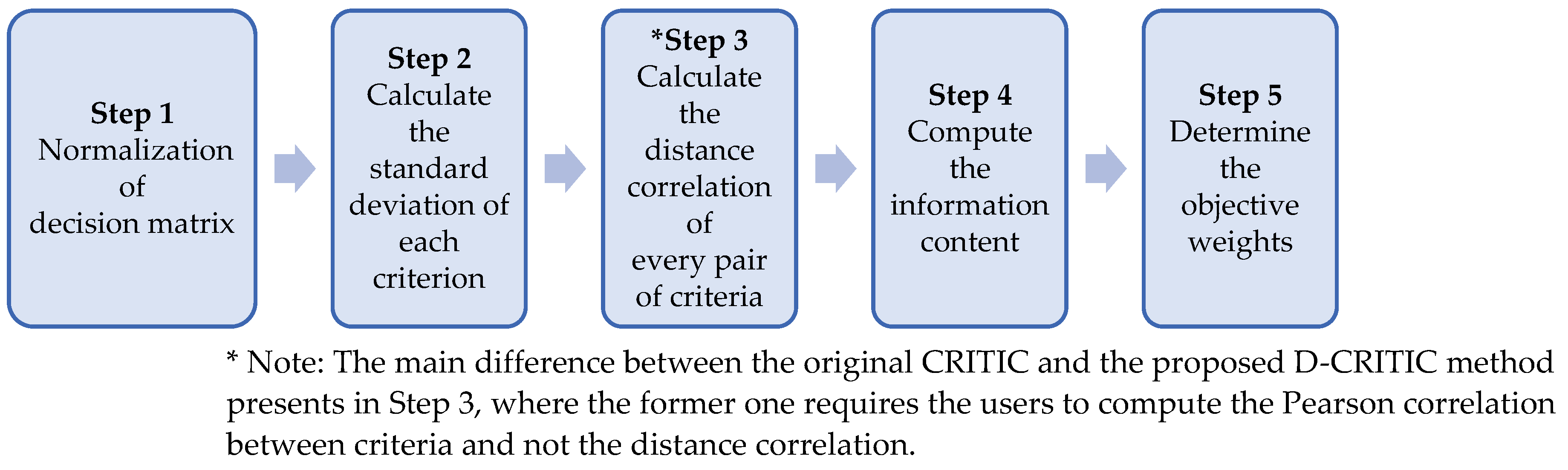
In fact, the limited number of studies on modified CRITIC methods implies that researchers may not have detected any serious issues with CRITIC’s fundamental components, suggesting that major modifications may not be needed. However, in the present study, we discovered that the original CRITIC method has a shortcoming in properly capturing the conflicting relationships between criteria, since it merely utilizes the Pearson correlation for this purpose. Studies indicate that this correlation does not always denote the actual relationships between criteria [43]. For instance, two criteria with a zero Pearson correlation coefficient may not be completely independent [44]. This undesirable situation occurs because the Pearson correlation detects only the linear relationship between two criteria and not the nonlinear relationship [45,46]. Thus, the validity of the weights computed by the original CRITIC method can be disputed.

Therefore, this research was motivated by the need for a modified CRITIC method that does not misrepresent the conflicting relationships between decision criteria. Proving that such a modified method can perform better than the original CRITIC method was another challenge that was addressed in this research.

1.2. Statement on Contributions

The key contribution of this research is twofold. First, in the context of the MCDM literature, we have introduced an improved version of the CRITIC method, namely D-CRITIC. D-CRITIC was developed by incorporating the idea of distance correlation into the original CRITIC method. Such a novel extension has not been reported in any of the studies relating to criteria weighting methods. The proposed D-CRITIC method has the merit of modelling the conflicting relationships between criteria more reliably with the aid of distance correlation. More importantly, this research has proven that D-CRITIC can produce a more valid set of criteria weights and ranks than the original CRITIC method. The introduction of D-CRITIC can also be regarded as an attempt to diversify the current literature, which is concentrated more on subjective weighting methods than on objective methods [47].

The second contribution of our research is linked to one of the tests conducted to validate the performance of D-CRITIC. Overall, we have conducted three different tests to compare the performance of the method. The purpose of the first test was to compare the degree of agreement of the criteria weights derived by D-CRITIC against four other weighting methods, including the original CRITIC method. Usually, the Pearson correlation test is conducted for this purpose [48,49]. However, we discovered that this test could deliver misleading results since the Pearson correlation is unable to capture a nonlinear association [50] between any two sets of weights. Therefore, we used the distance correlation test as an alternative approach to comparing the degree of agreement between different sets of criteria weights. The study is the first to offer a distance correlation test to measure the performance of different weighting methods.

In short, we employed the idea of distance correlation not only to develop a modified version of the CRITIC method but also to validate the performance of the modified method, that is, the D-CRITIC method.

2. The Proposed D-CRITIC Method

The proposed D-CRITIC method was developed by incorporating the idea of distance correlation into the original CRITIC method. All in all, as summarized in Figure 1, the application of D-CRITIC involves five crucial steps. A detailed explanation of each step is provided in the following sections.

• Normalization of the decision matrix (Step 1)
  The scores of different criteria are incommensurable as they are expressed in different measurement units or scales. Normalization is a process of transforming the scores into standard scales, which range between 0 and 1. In the proposed method, as a first step, we use Equation (2) for normalizing the scores available in the decision matrix.

  $$\overline{x_{ij}}=\frac{x_{ij}-x_j^{worst}}{x_j^{best}-x_j^{worst}},$$

  (2)

  where $\overline{x_{ij}}$ is the normalized score of alternative $i$ with respect to criterion $j$, $x_{ij}$ is the actual score of alternative $i$ with respect to criterion $j$, $x_j^{best}$ is the best score of criterion $j$, and $x_j^{worst}$ is the worst score of criterion $j$.
• Calculate the standard deviation of each criterion (Step 2)
  In the second step, the standard deviation of each criterion, $s_j$, is calculated using Equation (3). Note that $\overline{x_j}$ in Equation (2) is the mean score of criterion $j$ and that $m$ is the total number of alternatives.

  $$s_j=\sqrt{\frac{{\left({{\displaystyle \sum }}_{i=1}^m{x}_{ij}-\overline{x_j}\right)}^2}{m-1}},$$

  (3)

  where $\overline{x_j}$ is the mean score of criterion $j$ and $m$ is the total number of alternatives.
• Calculate the distance correlation of every pair of criteria (Step 3)
  The main difference between the proposed D-CRITIC and the original CRITIC method can be observed in the third step. In the original CRITIC method, the conflicting relationships between criteria are captured with the help of the Pearson correlation. However, as explained in Section 1.1, the Pearson correlation has the risk of inaccurately capturing the actual relationships between criteria. More precisely, two criteria with a zero Pearson correlation coefficient may not be completely independent. Accordingly, Székely et al. [43] introduced a new correlation measure, called distance correlation, that is zero if, and only if, the criteria are independent. Therefore, in the modified D-CRITIC method, the distance correlation is used as an alternative way to model the relationships, with the aim of minimizing the possible error in the final weights. Equation (4) defines the distance correlation between $c_j$ and $c_{j^{\prime }}$.

  $$dCor\left(c_j, c_{j^{\prime }}\right)=\frac{dCov\left(c_j, c_{j^{\prime }}\right)}{sqrt\left(dVar\left(c_j\right)dVar\left(c_{j^{\prime }}\right)\right)},$$

  (4)

  where $dCov\left(c_j,c_{j^{\prime }}\right)$ is the distance covariance between $c_j$ and $c_{j^{\prime }}$, $dVar\left(c_j\right)=dCov\left(c_j,c_j\right)$ is the distance variance of $c_j$, and $dVar\left(c_{j^{\prime }}\right)=dCov\left(c_{j^{\prime }},c_{j^{\prime }}\right)$ is the distance variance of $c_{j^{\prime }}$ [51]. The detailed steps of determining the distance correlation of every two criteria, $c_j$ and $c_{j^{\prime }}$, can be summarized as follows:
  • Step 3.1—Construct the Euclidean distance matrix of $c_j$ based on its scores associated with all the alternatives under consideration. Construct a similar matrix for $c_{j^{\prime }}$.
  • Step 3.2—Perform the following double-centring steps on each matrix, so that the row means, column means, and the overall mean of the elements in each matrix become zero: Deduct the row mean from each element; in the result, deduct the column mean from each element; in the result, add the matrix mean to each element.
  • Step 3.3—Multiply the double-centred matrices elementwise and calculate the average value of the elements from the resulting matrix, that is, the sum of elements divided by the total number of elements. The square root of this average value is the distance covariance of $c_j$ and $c_{j^{\prime }}$, that is, $dCov\left(c_j,c_{j^{\prime }}\right)$.
  • Step 3.4—Compute the distance variance of $c_j$, $dVar\left(c_j\right),$ and the distance variance of $c_{j^{\prime }}$, $dVar\left(c_{j^{\prime }}\right)$. Since $dVar\left(c_j\right)=dCov\left(c_j,c_j\right)$ and $dVar\left(c_{j^{\prime }}\right)=dCov\left(c_{j^{\prime }},c_{j^{\prime }}\right)$, these two values can be computed by repeating Steps 3.1–3.4.
  • Step 3.5—The available $dCov\left(c_j,c_{j^{,}}\right)$, $dVar\left(c_j\right)$, and aaaaa are substituted into Equation (4) to determine the distance correlation between $c_j$ and $c_{j^{\prime }}$, that is, $dCor\left(c_j,c_{j^{\prime }}\right)$.

At the end of this step, the symmetrical distance correlation matrix, $\left[dCov\left(c_j,c_{j^{\prime }}\right)\right]$, can be formed.

d.

Compute the information content (Step 4)

The amount of information contained in criterion $j$ is calculated by applying Equation (5).

$$I_j=s_j{{\displaystyle \sum }}_{j^{\prime }=1}^n(1-dCor\left(c_j,c_{j^{\prime }}\right)),$$

(5)

where $I_j$ denotes the information content of $c_j$.

e.

Determine the objective weights (Step 5)

The objective weight of criterion $j$ is determined using Equation (6).

$$w_j=\frac{I_j}{{{\displaystyle \sum }}_{j=1}^n{I}_j},$$

(6)

where $w_j$ is the objective weight of $c_j$.

3. Application of D-CRITIC to a Decision Problem

Many popular gadget websites provide a list of crucial criteria for smartphone selection. Some even rank these criteria from the most to the least important one. Since the smartphone market is becoming more and more competitive, providing such information will undoubtedly be helpful for the manufacturers to develop the right product strategies to sustain them in such a competitive marketplace.

There are several MCDM-based studies conducted to determine the weights and ranks of smartphone criteria scientifically. For instance, Peaw and Mustafa [52] evaluated various smartphone criteria, including the dimension and screen resolution, using the combination of AHP and Data Envelopment Analysis. Meanwhile, Ho et al. [53] analyzed the responses collected from a sample of customers using a modified AHP to evaluate eight selected criteria, which include the display quality, camera, and price. In another study, Okfalisa et al. [54] applied both the fuzzy AHP and fuzzy analytical network process for a similar smartphone criteria evaluation purpose.

Surprisingly, most of the previous studies on the evaluation of smartphone criteria were more focused on using subjective weighting methods, e.g., AHP. In this section, we are interested in establishing that the objective weighting methods, particularly the D-CRITIC method, can be used as a potential alternative tool to determine the weights and ranks of smartphone criteria.

Table 1. Decision matrix of smartphone models.

Model/Criterion	${\mathit{c}}_1$ (Nonbeneficial)	${\mathit{c}}_2$ (Beneficial)	${\mathit{c}}_3$ (Beneficial)	${\mathit{c}}_4$ (Nonbeneficial)	${\mathit{c}}_5$ (Nonbeneficial)
Model A	649	4.7	326	7.1	143
Model B	749	5.5	401	7.3	192
Model C	740	5.7	520	7.6	171
Model D	400	5.7	520	11.1	179
Model E	600	5.5	538	8.9	152

Source: https://www.trendhunter.com/trends/smartphone-guide (accessed on 2 November 2020).

shows the decision matrix of five smartphone models that were compared according to five criteria, namely the base price measured in dollars ($c_1)$, the screen size measured in inches ($c_2)$, the pixel density measured in pixels per centimetre ($c_3)$, the thickness measured in millimetres ($c_4)$, and the mass measured in grams ($c_5)$. The smartphone models were renamed as Models A, B, C, D, and E for confidentiality.

Note that the actual smartphone comparison data obtained from https://www.trendhunter.com/trends/smartphone-guide (accessed on 2 November 2020) consists of ten criteria. However, we had to drop five criteria from further analysis due to some reasons. The operating system, processor, and special feature criteria were removed since they are qualitative in nature, making them not compatible as input criteria for D-CRITIC. A similar reason applied to storage criterion as the data are mixed with quantitative and qualitative values, besides the fact that there is no single, fixed value with respect to each smartphone. The battery criterion was removed due to the issue of data incompleteness. To simplify, after taking into consideration the suitability of the criteria data with the proposed method, only five criteria were finalised for the analysis.

Table 2. Normalized decision matrix.

Model/Criterion	${\mathit{c}}_1$	${\mathit{c}}_2$	${\mathit{c}}_3$	${\mathit{c}}_4$	${\mathit{c}}_5$
A	0.2865	0	0	1	1
B	0	0.8000	0.3538	0.9500	0
C	0.0258	1	0.9151	0.8750	0.4286
D	1	1	0.9151	0	0.2653
E	0.4269	0.8000	1	0.5500	0.8163
Standard deviation	0.4062	0.4147	0.4394	0.4161	0.4063

is the normalized decision matrix derived from Equation (1). The worst and best values of each criterion were carefully identified before applying Equation (1). Note that the base price, thickness, and mass are nonbeneficial criteria, whereas the remaining are beneficial criteria. Therefore, for the case of a nonbeneficial criterion, the lowest value is considered the most preferred or best value. In contrast, for a beneficial criterion, as usual, the highest value is considered the best one. For instance, the best and worst values for the base price are $400 and $749, respectively. Meanwhile, for screen size, 5.7 in. and 4.7 in. are considered the best and the worst value, respectively. The standard deviation value of each criterion, which was computed using Equation (2), is also presented in the same table. These values suggest that the data pattern of pixel density has the highest contrast, followed by thickness, screen size, mass, and base price. However, at this level, it is too early for us to identify pixel density as the essential criterion, for the following two reasons:

• The standard deviation values, which are relatively close to each other, do not show a clear distinction in terms of their contrast intensity, so we are unable to make a concrete decision about the importance of the criteria.
• The relationships held by the criteria are yet to be considered.

The analysis, therefore, proceeded by computing the distance correlation measures of the criteria.

Table 3. Distance correlation matrix.

Criterion	${\mathit{c}}_1$	${\mathit{c}}_2$	${\mathit{c}}_3$	${\mathit{c}}_4$	${\mathit{c}}_5$
$c_1$	1	0.4777	0.5114	0.9437	0.6229
$c_2$	0.4777	1	0.8465	0.5499	0.7564
$c_3$	0.5114	0.8465	1	0.6957	0.6043
$c_4$	0.9437	0.5499	0.6957	1	0.5027
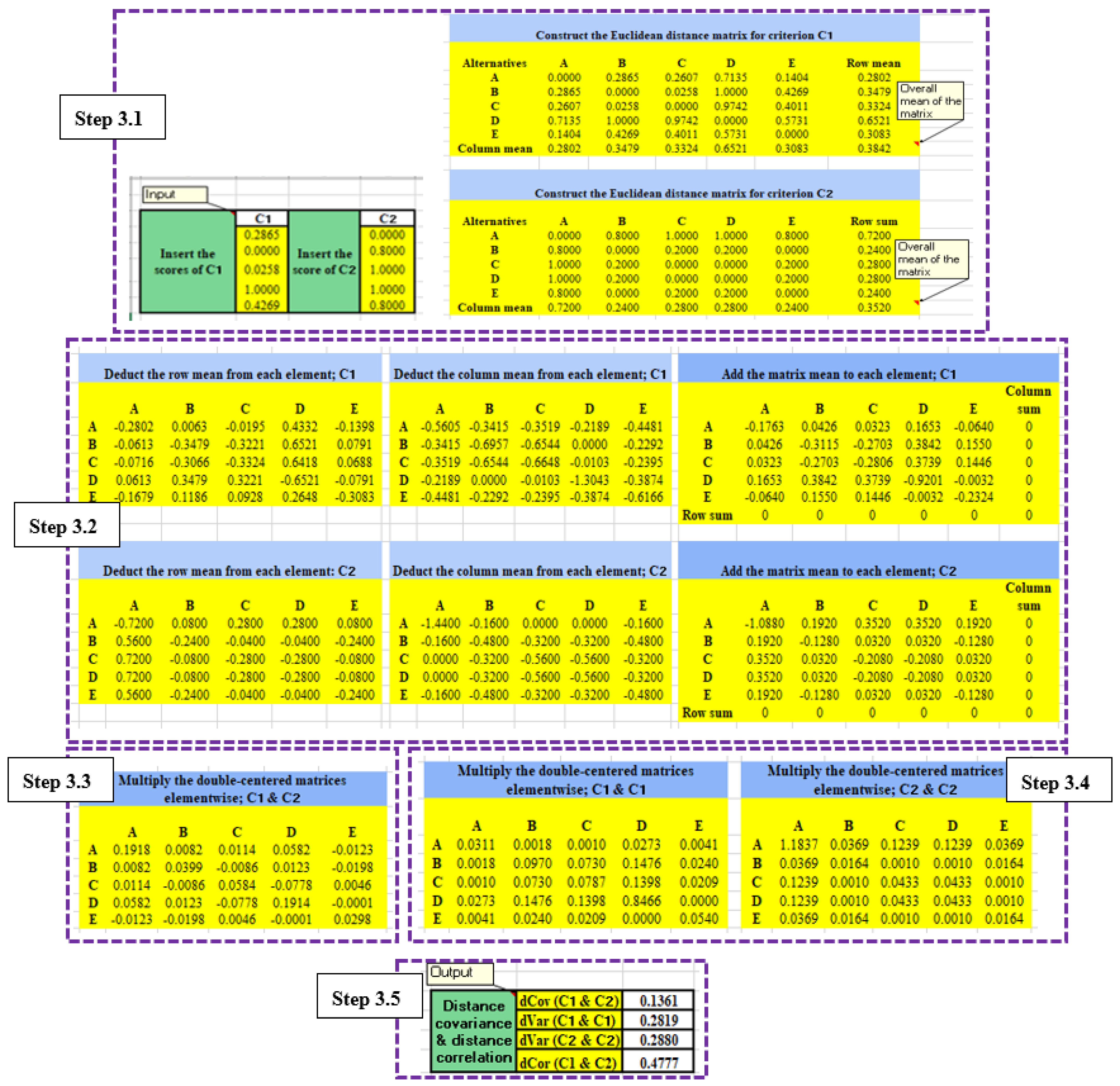
$c_5$	0.6229	0.7564	0.6043	0.5027	1

depicts the distance correlation matrix of the criteria. To facilitate a better understanding, we present in Appendix A an example of calculating the distance correlation for $c_1$ and $c_2$, $Dcor \left(c_2, c_2\right)$. Based on Table 3, the highest distance correlation measure is noticed between the base price and the thickness (i.e., 0.9437), indicating a strong redundancy between both criteria. It also appears that the mass criterion does not largely overlap with any other criterion since none of the measures are above 0.8. This situation suggests that the mass could be identified as the most important criterion by the end of the analysis.

Table 4. Information content and weight of each criterion.

Criterion	${\mathit{c}}_1$	${\mathit{c}}_2$	${\mathit{c}}_3$	${\mathit{c}}_4$	${\mathit{c}}_5$
Information content	0.5867	0.5680	0.5898	0.5442	0.6149
Weight	0.2021	0.1956	0.2031	0.1874	0.2118

shows the information content and the weight of each criterion determined using Equations (5) and (6), respectively. In short, as expected, D-CRITIC identifies $c_5$ as the most important criterion with a weight score of 0.2118, followed by criteria $c_3$, $c_1$, $c_2$, and $c_4$.

4. Comparison Analysis

In this section, the weights of the same five smartphone criteria were determined using four other objective methods to validate the performance of D-CRITIC. Those methods were Hwang’s entropy-based method [25], CILOS [28], IDOCRIW [28], and not to mention the original CRITIC method [27]. The entropy-based method was chosen because of its long existence and widespread application in real problems, apart from its ability to capture the contrast intensity of each criterion. On the other hand, the recently developed CILOS and IDOCRIW methods were selected because they consider the criteria’s impact loss element in the determination of the weights.

We had to exclude subjective weighting methods, which usually use different input types, from our comparison analysis to ensure an apples-to-apples comparison. In this study, such a fair comparison can be assured by only considering similar objective methods since they use the same input, i.e., the data in the decision matrix. Indeed, many earlier studies, which introduced a new or modified objective weighting method, presented their comparison analysis similarly. For instance, the study that introduced the original CRITIC method compared the method with only two different objective methods, and not with any other subjective methods [27].

Table 5. Results of different methods.

Criterion	Entropy		CILOS		IDOCRIW		CRITIC		D-CRITIC
	Weight	Rank	Weight	Rank	Weight	Rank	Weight	Rank	Weight	Rank
$c_1$	0.3481	1	0.0738	5	0.1465	3	0.1872	3	0.2021	3
$c_2$	0.1360	5	0.3864	1	0.2996	2	0.1838	4	0.1956	4
$c_3$	0.1690	3	0.0997	4	0.0960	5	0.1691	5	0.2031	2
$c_4$	0.1463	4	0.1467	3	0.1223	4	0.2599	1	0.1874	5
$c_5$	0.2006	2	0.2934	2	0.3355	1	0.2000	2	0.2118	1

shows the weights and ranks obtained by all five methods, including D-CRITIC. Meanwhile, Figure 2 offers a visual summary of the variances between the weights determined by those methods. The complete calculation associated with each method can be found in the provided Supplementary File. Based on these different results, the performance of D-CRITIC was then compared by conducting the following tests: (a) the distance correlation test, (b) the Spearman rank-order correlation test, and (c) the symmetric mean absolute percentage error square error (sMAPE) test.

4.1. Distance Correlation Test

The degree of agreement or consistency between two sets of weights, resulting from two different methods, is usually measured using the Pearson correlation [55]. However, as explained in Section 1.1, the Pearson correlation coefficient could inaccurately represent the correlation between two data arrays. Therefore, the distance correlation was used to measure consistency.

Table 6. Distance correlation between criteria weights.

Method	Entropy	CILOS	IDOCRIW	CRITIC	D-CRITIC
Entropy	1	0.5897	0.4609	0.4658	0.6336
CILOS	0.5897	1	0.9527	0.4968	0.5975
IDOCRIW	0.4609	0.9527	1	0.5057	0.5919
CRITIC	0.4658	0.4968	0.5057	1	0.8186
D-CRITIC	0.6336	0.5975	0.5919	0.8186	1
Average	0.6300	0.7273	0.7022	0.6574	0.7283

shows the computed distance correlation between every two different sets of weights. Table 6 also shows the average correlation score of each method.

4.2. Spearman Rank-Order Correlation Test

The Spearman rank-order correlation test is a popular tool for measuring the degree of agreement between two different sets of ranks [56,57]. We therefore used this test to assess the consistency across the criteria ranks obtained by all five methods. This correlation test was chosen due to its appropriateness as a non-parametric test that efficiently measures the association between two different ordinal data arrays [58], apart from its computational simplicity [59].

Table 7. Spearman rank-order correlation between criteria ranks.

Method	Entropy	CILOS	IDOCRIW	CRITIC	D-CRITIC
Entropy	1	−0.7000	0.1000	0.1000	0.6000
CILOS	−0.7000	1	0.6000	0.1000	−0.1000
IDOCRIW	0.1000	0.6000	1	0.3000	0.3000
CRITIC	0.1000	0.1000	0.3000	1	−0.3000
D-CRITIC	0.6000	−0.1000	0.3000	−0.3000	1
Average	0.2200	0.1800	0.4600	0.2400	0.3000

reports the Spearman rank-order correlation between every pair of methods, including the average Spearman rank-order correlation score of each method.

4.3. sMAPE Test

There exist many error metrics that can be used to quantify the degree of difference between a group of estimated values and actual values, e.g., mean absolute error, mean squared error, root mean square error, mean absolute percentage error (MAPE), and symmetric MAPE (sMAPE). The literature suggests that these error metrics can also be employed to test the accuracy of the results generated by different MCDM methods [60]. Usually, the lower the error value, the higher the accuracy of the method. A set of actual values is needed to enable the use of any error metrics.

In this research, Equation (7), based on the geometric mean, was used to aggregate the weights from different methods.

$$w_j=\frac{\left(\widehat{w_j}, entropy\right)·\left(\widehat{w_j}, CILOS\right)·\left(\widehat{w_j}, IDOCRIW\right)·\left(\widehat{w_j}, CRITIC\right)·\left(\widehat{w_j}, D-CRITIC\right)}{{{\displaystyle \sum }}_{j=1}^n\left[\left(\widehat{w_j}, entropy\right)·\left(\widehat{w_j}, CILOS\right)·\left(\widehat{w_j}, IDOCRIW\right)·\left(\widehat{w_j}, CRITIC\right)·\left(\widehat{w_j}, D-CRITIC\right)\right]},$$

(7)

where $w_j$ is the final aggregated weight of criterion $j$, $\widehat{w_j}$ is the weight of criterion $j$ estimated using each method, and $j=$ {1,2,3,4,5}.

By treating these aggregated weights as the actual ones, Equation (8) was then used to identify the sMAPE of each method. Out of many metrics, sMAPE was chosen because unlike MAPE, it does not impose a larger penalty for negative error (when the estimated value is higher than actual value) than for positive error [61,62].

$$sMAPE=\frac{100\%}{n}{{\displaystyle \sum }}_{j=1}^n\frac{\left|w_j-\widehat{w_j}\right|}{\left(w_j+\widehat{w_j}\right)/2}.$$

(8)

Table 8. Aggregated weight of each criterion.

${\mathit{c}}_1$	${\mathit{c}}_2$	${\mathit{c}}_3$	${\mathit{c}}_4$	${\mathit{c}}_5$
0.1802	0.2375	0.1493	0.1763	0.2568

shows the aggregated weights, and

Table 9. sMAPE of each method.

Entropy	CILOS	IDOCRIW	CRITIC	D-CRITIC
34.6994%	40.6001%	29.9940%	20.9825%	17.3267%

illustrates the sMAPE of each method compared with the aggregated weights. Meanwhile, Figure 3 summarizes the performance of each method based on its average distance correlation score, average Spearman rank-order correlation score, and sMAPE.

5. Sensitivity Analysis

In this section, we furthered our investigation to understand the robustness of the proposed D-CRITIC method. Robustness explains the steadiness of the results produced by a method. As far as MCDM literature is concerned, sensitivity analysis has always been a popular choice of tool to examine the robustness of various MCDM methods, e.g., [63,64]. Generally, a sensitivity analysis explores how a little change in the input parameters could affect the output resulting from a method.

Therefore, in this study, the sensitivity analysis was conducted with the aim of understanding how the variation in the size of the decision matrix will affect the criteria weights and ranks estimated by D-CRITIC. Since the weights estimated by D-CRITIC are subjected to the data structure in the decision matrix, it is then rational to analyze the effect of different dimensions of the decision matrix on the criteria weights and ranks.

We commenced the analysis by generating ten different scenarios. These scenarios were created by merely amending the existing decision matrix that comprises data of five alternatives, i.e., smartphones ($m=5$). The amendment was done so that at the end, we would have slightly smaller ($m=4$) and larger ($m=6$) decision matrices than the actual ones. For the first five scenarios, we eliminated one alternative while retaining the other four. Meanwhile, for the next five scenarios, we duplicated the data of one selected alternative so that each scenario would have a decision matrix with $m=6$. More details about these ten scenarios are summarized in

Table 10. The scenarios for sensitivity analysis.

Scenario	Amendment Done	Decision Matrix	Normalized Decision Matrix
Scenario 1 (Sc1)	Removed the data of Model B
Scenario 2 (Sc2)	Removed the data of Model C
Scenario 3 (Sc3)	Removed the data of Model D
Scenario 4 (Sc4)	Removed the data of Model E
Scenario 5 (Sc5)	Removed the data of Model A
Scenario 6 (Sc6)	Duplicated the data of Model A
Scenario 7 (Sc7)	Duplicated the data of Model B
Scenario 8 (Sc8)	Duplicated the data of Model C
Scenario 9 (Sc9)	Duplicated the data of Model D
Scenario 10 (Sc10)	Duplicated the data of Model E

.

The D-CRITIC method was then applied to each scenario.

Table 11. Criteria weights resulting from different scenarios.

Criterion	Sc1	Sc2	Sc3	Sc4	Sc5	Sc6	Sc7	Sc8	Sc9	Sc10
$c_1$	0.2242	0.1657	0.2071	0.2309	0.1836	0.1898	0.1896	0.2125	0.2245	0.1880
$c_2$	0.1897	0.2018	0.2021	0.1849	0.3058	0.2039	0.2008	0.1925	0.1805	0.2015
$c_3$	0.2227	0.1868	0.2091	0.1898	0.1826	0.2114	0.1901	0.2110	0.1947	0.2146
$c_4$	0.1905	0.1710	0.1999	0.2180	0.1669	0.1825	0.1857	0.1955	0.2031	0.1719
$c_5$	0.1729	0.2747	0.1818	0.1765	0.1611	0.2123	0.2338	0.1886	0.1973	0.2240

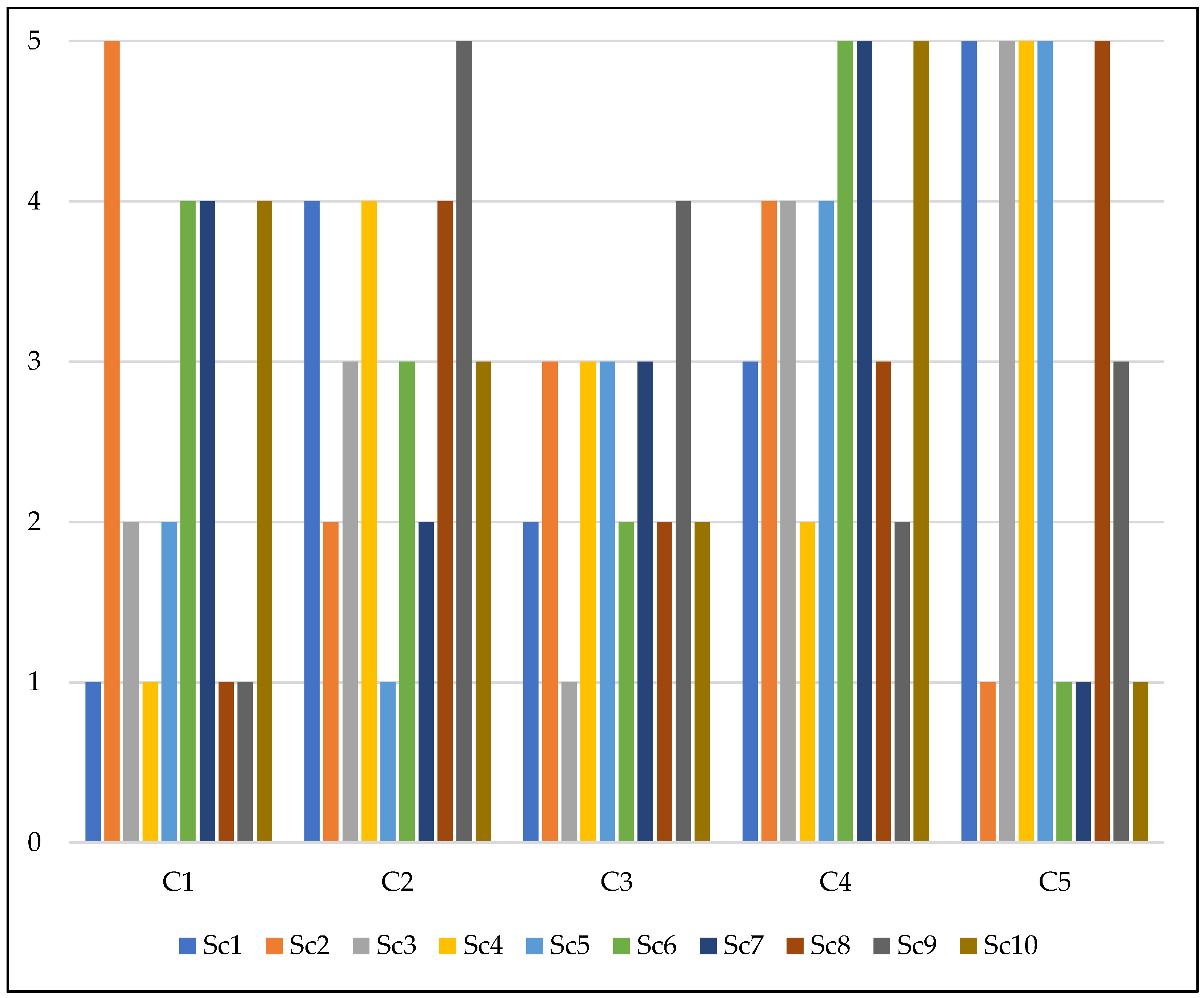
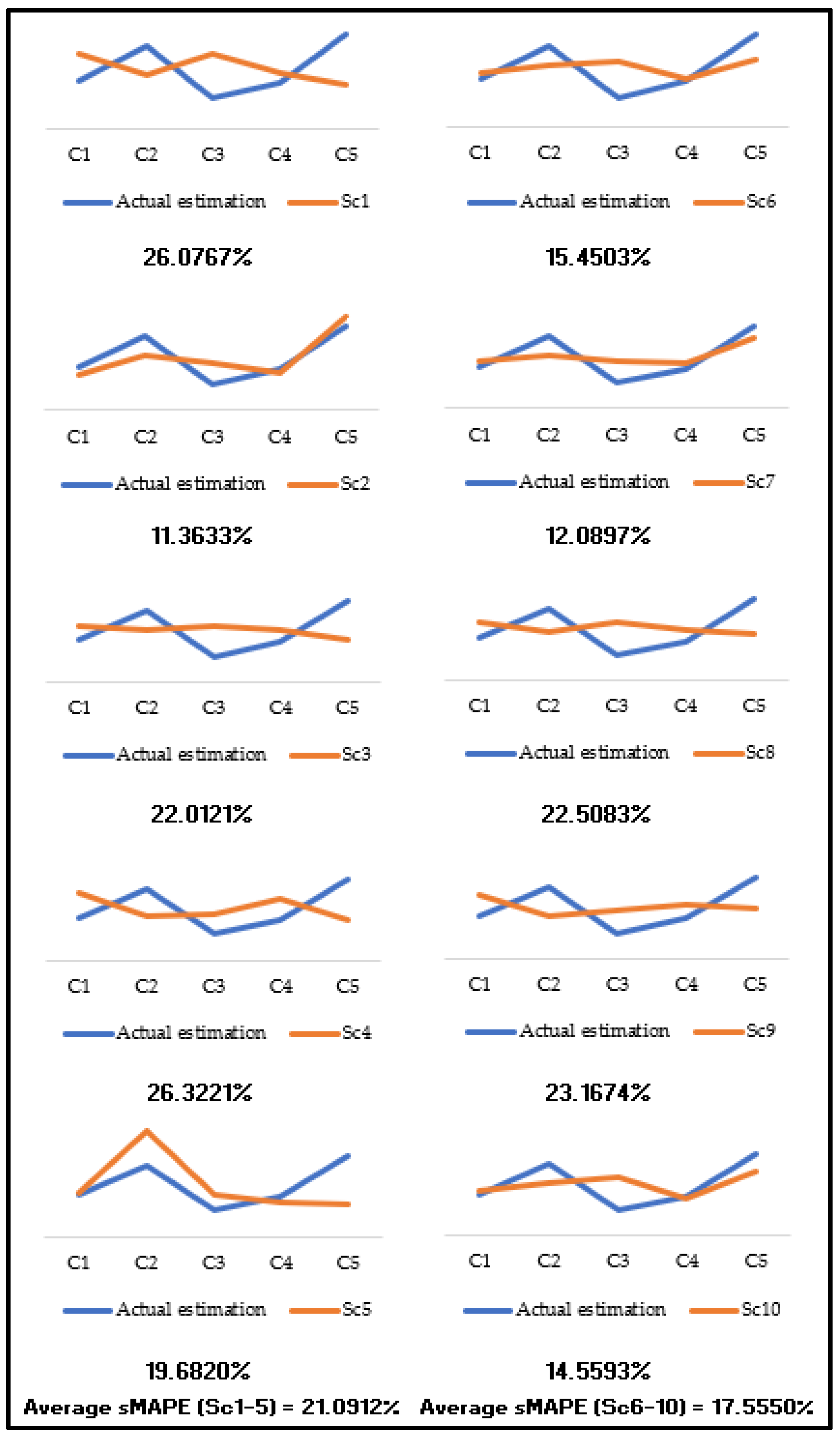
summarizes the criteria weights resulting from every different scenario. Figure 4 displays the variations observed in the ranking of each criterion across the ten scenarios. Meanwhile, Figure 5 displays the comparison between the criteria weights of each scenario against the weights estimated from the actual decision matrix, together with the sMAPE of each scenario and average sMAPE for Sc1-Sc5 and Sc6-Sc10. On the other hand,

Table 12. Criteria ranks of each scenario vs. actual ranks.

	$\mathbf{Scenarios}\mathbf{with}\mathit{m}=4$					$\mathbf{Actual}\mathbf{scenario}\mathbf{with}\mathit{m}=5$	$\mathbf{Scenarios}\mathbf{with}\mathit{m}=6$
Criteria	Sc1	Sc2	Sc3	Sc4	Sc5	Actual Estimation	Sc6	Sc7	Sc8	Sc9	Sc10
$c_1$	1	5	2	1	2	3	4	4	1	1	4
$c_2$	4	2	3	4	1	4	3	2	4	5	3
$c_3$	2	3	1	3	3	2	2	3	2	4	2
$c_4$	3	4	4	2	4	5	5	5	3	2	5
$c_5$	5	1	5	5	5	1	1	1	5	3	1
	Total unaffected ranks = 4						Total unaffected ranks = 10

Note: The green highlight indicates that the ranking of the criterion under that specific scenario has remained unaffected when compared to the actual ranks.

provides a comparison of the criteria ranks from all ten scenarios against the actual estimation. Note that the green highlight in Table 12 indicates that the ranking of the criterion under that specific scenario has remained unaffected when compared to the actual ranks.

6. Discussion and Conclusions

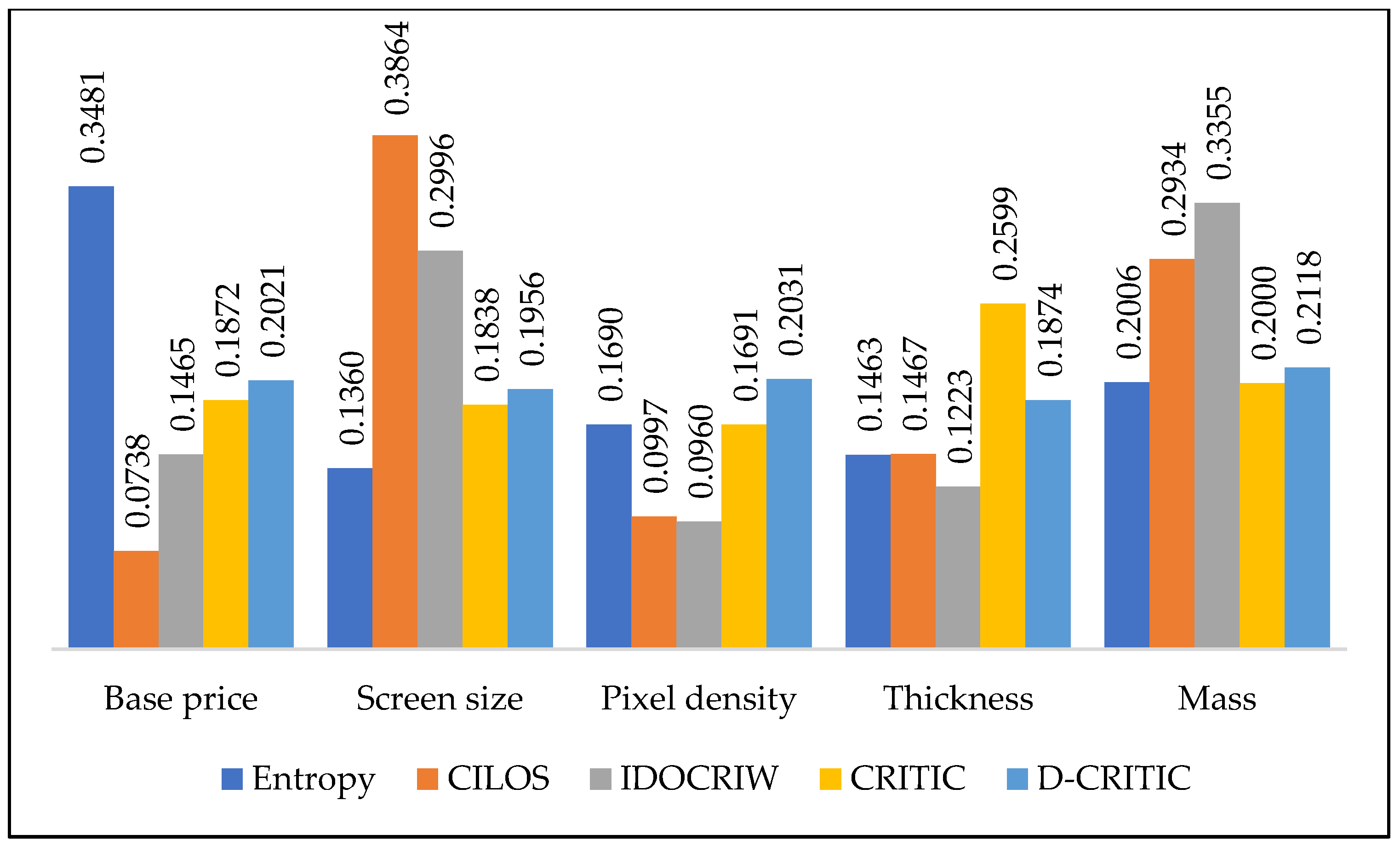
The proposed D-CRITIC method and four other objective weighting methods were applied to a smartphone criteria evaluation problem to demonstrate the workability of D-CRITIC. D-CRITIC identified mass as the most salient criterion with a weight of 0.2118 (see Table 5), followed by pixel density (0.2031), base price (0.2021), screen size (0.1956), and thickness (0.1874). Interestingly, two other methods, namely CILOS and IDOCRIW, also reported mass as the most critical smartphone criterion. We realize that the results of D-CRITIC are consistent with the findings reported in several past studies. Yildiz and Ergul [65] applied a subjective weighting method, i.e., ANP, for evaluating a long list of smartphone selection criteria and proved that the mass of a smartphone is more important than its thickness. Lee et al. [66] indeed claimed that mass is an essential criterion for an ergonomic smartphone since it helps in providing the expected one-handed grip comfort to users. In another study conducted by Mishra et al. [67], similar to the results of D-CRITIC, it was reported that pixel density is more crucial than screen size. In fact, Zhu et al. [68] stated that the specifications of the camera and the quality of taken photos are becoming dominant criteria for customers purchasing smartphones. Many smartphone manufacturers also tend to promote their smartphones by emphasizing the strength of their smartphone camera specifications, including the pixel density.

It could be surprising to notice that D-CRITIC did not identify price as the most important smartphone selection criterion. Similar to our findings, Bhalla et al. [69] also recently reported that price has less effect on a customer’s buying decision when compared to other physical features of a smartphone. In a similar vein, Osman et al. [70] claimed that customers nowadays care more about the physical features of a smartphone and are willing to pay more in exchange for better features. More importantly, from the MCDM perspective, the price data of the five smartphone models considered in this study are found not to vary too much (with the lowest standard deviation value), indicating that this specific criterion has the lowest degree of contrast intensity and least information to tell. Such a data pattern further strengthens the logic as to why D-CRITIC did not identify price as the most crucial criterion.

On the other hand, a somewhat uniform line for D-CRITIC compared with the other lines (see Figure 1) indicates that D-CRITIC assigns weights that are relatively close to each other. In other words, it appears that D-CRITIC concludes that all five smartphone criteria hold a similar degree of importance, with only marginal differences. Although the weights estimated by D-CRITIC are relatively close, it has to be emphasized that they are still distinct enough to enable a decent ranking on the criteria. It is acceptable to have relatively close weights since, in some situations, that could be the actual case. For instance, Suh et al. [71], who used an integrated weighting method to evaluate eight mobile service criteria, discovered that the computed weights did not vary too much and merely ranged between 0.0870 and 0.1780.

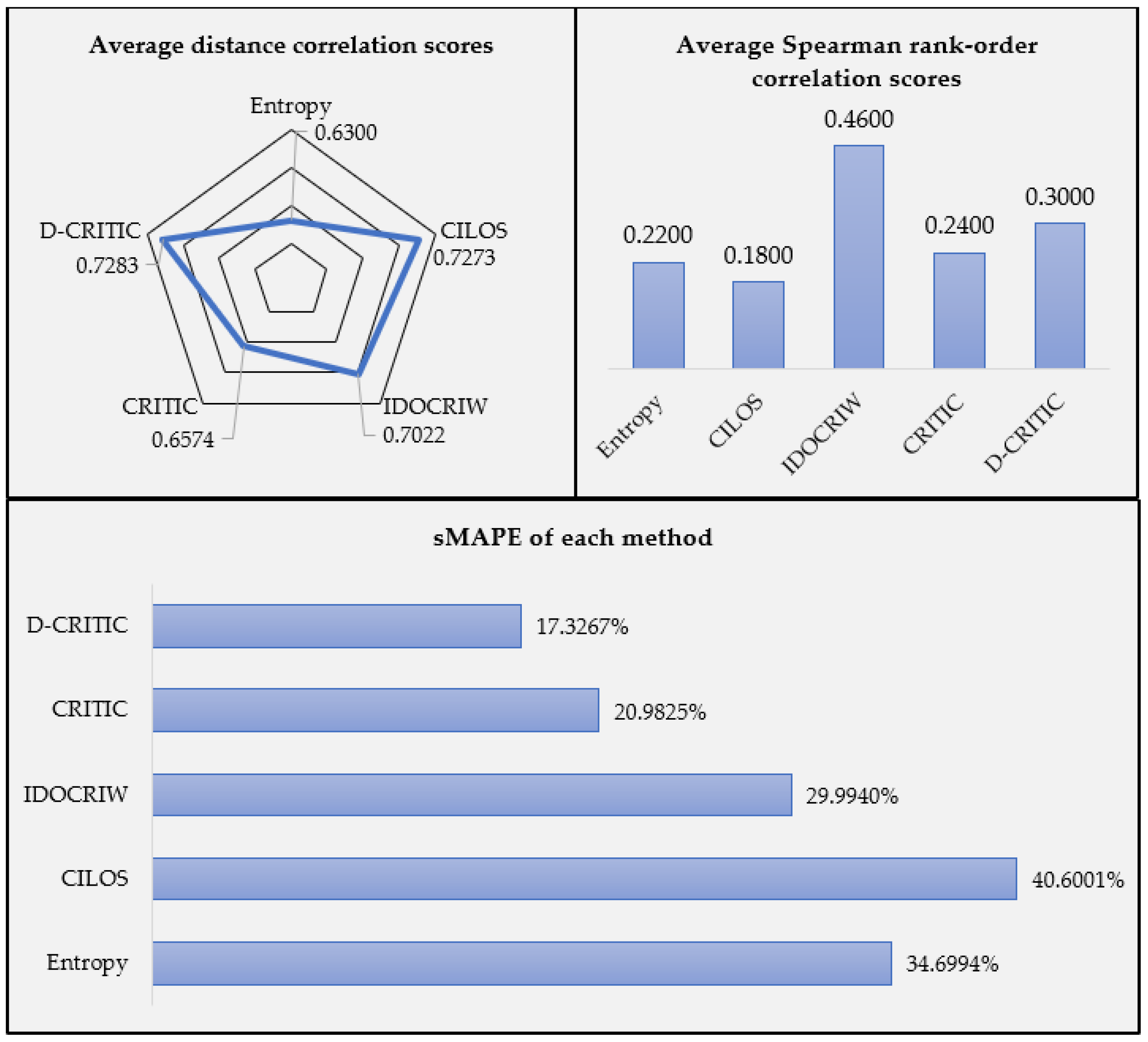
More importantly, further analyses (the distance correlation test, the Spearman rank-order correlation, the sMAPE test, and the sensitivity analysis) have provided obvious evidence that the weights estimated by D-CRITIC are more acceptable than those of other methods.

The distance correlation test reveals that the set of weights derived by the D-CRITIC method is strongly consistent with the sets of weights produced by the other methods since all the coefficient values are above 0.6. The highest consistency is reported for the original CRITIC method, with a coefficient value of 0.8186. This finding is undoubtedly the result of the similarity between the two methods in determining the criteria weights. More specifically, unlike other methods, both methods capture the contrast intensity and the conflicting nature of the criteria while determining the weights. However, overall, the set of weights produced by D-CRITIC has the highest degree of consistency compared with the weights produced by the other four methods; that is, D-CRITIC yielded the largest average distance correlation score (0.7283). The second most consistent weights were derived by CILOS (0.7273), followed by IDOCRIW (0.7022), CRITIC (0.6574), and the entropy-based method (0.6300).

On the other hand, the Spearman rank-order correlation test reveals that the most consistent criteria ranks, which agree well with the other four sets of criteria ranks, resulted from the IDOCRIW method. Interestingly, as in the case of criteria weights, it appears that the set of ranks derived by D-CRITIC is more consistent than that derived by CRITIC, since the former has a higher average Spearman rank-order correlation score (0.3000).

Besides, the sMAPE test shows that D-CRITIC has estimated the most accurate criteria weights since the method obtained the lowest sMAPE value, that is, 17.3267%, when compared with the aggregated weights. The original CRITIC method is reported as the second most accurate method with an sMAPE value of 20.9825%. The test also indicates that the entropy method produced the second-least accurate estimates because, unlike D-CRITIC and CRITIC, the entropy method considers only the contrast intensity of the criteria.

To sum up, based on Figure 3, it can be claimed that D-CRITIC has a better performance than the original CRITIC method. The D-CRITIC method is proven to have the ability to produce a more valid set of criteria weights and ranks. The results support the initial argument made in Section 1.1 that the weights determined by the CRITIC method could be flawed since it misrepresents conflicting relationships between criteria. This shortcoming is minimized in the D-CRITIC method, mainly with the aid of distance correlation.

On the other hand, the results in Table 11 and Figure 4 clearly show that a little modification in the size of the decision matrix or the data structure, which was done through ten different scenarios, have caused changes to the weights or ranking of criteria estimated from the actual decision matrix. These changes prove that the D-CRITIC method results are sensitive to the variations in the size of the decision matrix. This situation is caused by the integrated distance correlation measures. Unlike the Pearson correlation, distance correlation is not only more responsive to the change in the amount of data, but at the same time, it is more sensitive to the presence of both linear and non-linear associations between data vectors.

However, it can be claimed that D-CRITIC can produce more stable criteria weights with a larger decision matrix. This quality is evident based on Figure 5, where it appears that weights generated by Sc6, Sc7, Sc8, Sc9, and Sc10 are more consistent with the actual estimation compared to Sc1, Sc2, Sc3, Sc4, and Sc5. Furthermore, the lower average sMAPE value for Sc6–Sc10, i.e., 17.5550%, in general, suggests that weights estimated via a larger decision matrix have better proximity to the actual estimation. It has to be reiterated that the decision matrix of Sc1–Sc5 only comprises four alternatives, whereas six alternatives make up the decision matrix of Sc6–Sc10.

In terms of the criteria ranks, few scenarios have generated ranks that tally with the actual estimation. For instance, $c_5$, which was identified as the most important criterion, has also been ranked first in Sc2, Sc6, Sc7, and Sc10. Besides, $c_4$, which was reported as the least important criterion, has remained at the same fifth rank in Sc6, Sc7, and Sc10. However, based on the number of green boxes distributed between Sc1-Sc5 and Sc6–Sc10, we can specifically claim that the ranks derived from larger decision matrices are more consistent with the actual estimation. All in all, the sensitivity analysis reveals that D-CRITIC has the tendency to deliver more stable criteria weights and ranks with a larger decision matrix, or in other words, if the decision problem involves a larger set of alternatives.

7. Limitations and Recommendations

Our research has two main limitations that should be addressed in future studies. The first limitation relates to the computational load of D-CRITIC. The method is more computationally demanding than the original CRITIC method since D-CRITIC is based on distance correlation. The original calculation of distance correlation presented in this paper can lead to a more complex procedure when a larger number of alternatives is involved. Huo and Székely [72] claimed that the computational complexity of distance correlation could be as high as a constant multiplied by $m^2$ (i.e., $O\ast m^2$), where $m$ denotes the number of alternatives. Future studies, therefore, may consider developing and using a simpler algorithm to calculate distance correlation prior to applying D-CRITIC.

The second limitation is that the proposed D-CRITIC method derives the weights merely by analyzing the data structure in the decision matrix without considering experts’ inputs. Although it has the advantage of minimizing the possible bias caused by human judgment, it may also disregard the valuable inputs from experienced experts. Thus, in the future, the users of D-CRITIC may consider using the method together with other subjective weighting methods, so that the final criteria weights can be determined by utilizing the benefits of both objective and subjective methods.

References

1. Sitorus, F.; Cilliers, J.J.; Brito-Parada, P.R. Multi-criteria decision making for the choice problem in mining and mineral processing: Applications and trends. Expert Syst. Appl. 2019, 121, 393–417. [Google Scholar] [CrossRef]
2. Parameshwaran, R.; Kumar, S.P.; Saravanakumar, K. An integrated fuzzy MCDM based approach for robot selection considering objective and subjective criteria. Appl. Soft Comput. 2015, 26, 31–41. [Google Scholar] [CrossRef]
3. Jankowski, P. Integrating geographical information systems and multiple criteria decision-making methods. Int. J. Geogr. Inf. Syst. 1995, 9, 251–273. [Google Scholar] [CrossRef]
4. Saad, R.M.; Ahmad, M.Z.; Abu, M.S.; Jusoh, M.S. Hamming Distance Method with Subjective and Objective Weights for Personnel Selection. Sci. World J. 2014, 2014, 865495. [Google Scholar] [CrossRef] [PubMed]
5. Krishnan, A.R.; Kasim, M.M.; Abu Bakar, E.M.N.E. A Short Survey on the Usage of Choquet Integral and its Associated Fuzzy Measure in Multiple Attribute Analysis. Procedia Comput. Sci. 2015, 59, 427–434. [Google Scholar] [CrossRef] [Green Version]
6. Wang, T.C.; Da Lee, H. Developing a fuzzy TOPSIS approach based on subjective weights and objective weights. Expert Syst. Appl. 2009, 36, 8980–8985. [Google Scholar] [CrossRef]
7. Krylovas, A.; Dadelienė, R.; Kosareva, N.; Dadelo, S. Comparative Evaluation and Ranking of the European Countries Based on the Interdependence between Human Development and Internal Security Indicators. Mathematics 2019, 7, 293. [Google Scholar] [CrossRef] [Green Version]
8. Deng, H.; Yeh, C.H.; Willis, R.J. Inter-company comparison using modified TOPSIS with objective weights. Comput. Oper. Res. 2000, 27, 963–973. [Google Scholar] [CrossRef]
9. Hovanov, N.V.; Kolari, J.W.; Sokolov, M. Deriving weights from general pairwise comparison matrices. Math. Soc. Sci. 2008, 55, 205–220. [Google Scholar] [CrossRef]
10. Saaty, T.L.; Kearns, K.P. The Analytic Hierarchy Process; Elsevier BV: Amsterdam, The Netherlands, 1985; pp. 19–62. [Google Scholar]
11. Keršulienė, V.; Zavadskas, E.K.; Turskis, Z. Racionalaus ginču̧ sprendimo būdo nustatymas taikant nauja̧ kriteriju̧ svoriu̧ nustatymo metoda̧, pagri̧sta̧ nuosekliu laipsnišku poriniu kriteriju̧ santykinės svarbos lyginimu. J. Bus. Econ. Manag. 2010, 11, 243–258. [Google Scholar] [CrossRef]
12. Krylovas, A.; Zavadskas, E.K.; Kosareva, N.; Dadelo, S. New KEMIRA Method for Determining Criteria Priority and Weights in Solving MCDM Problem. Int. J. Inf. Technol. Decis. Mak. 2014, 13, 1119–1133. [Google Scholar] [CrossRef]
13. Simos, J. Évaluer L’impact sur L’environnement. Une Approche Originale par L’analyse Multicritère et la Négotiation [Environmental Impact Assessment. An Original Approach for Multi-Criteria Analysis and Negociation]; Presses Polytechniques et Universitaires Romandes: Lausanne, Switzerland, 1990. [Google Scholar]
14. Danielson, M.; Ekenberg, L. An improvement to swing techniques for elicitation in MCDM methods. Knowl. Based Syst. 2019, 168, 70–79. [Google Scholar] [CrossRef]
15. Stanujkic, D.; Zavadskas, E.K.; Karabasevic, D.; Smarandache, F.; Turskis, Z. The use of the pivot pairwise relative criteria importance assessment method for determining the weights of criteria. Rom. J. Econ. Forecast. 2017, 20, 116–133. [Google Scholar] [CrossRef]
16. Pamučar, D.; Stević, Ž.; Sremac, S. A New Model for Determining Weight Coefficients of Criteria in MCDM Models: Full Consistency Method (FUCOM). Symmetry 2018, 10, 393. [Google Scholar] [CrossRef] [Green Version]
17. Fontela, E. Structural Analysis of the World Problematique: (Methods); Battelle Geneva Research Centre: Geneva, Switzerland, 1974. [Google Scholar]
18. Odu, G.O. Weighting methods for multi-criteria decision making technique. J. Appl. Sci. Environ. Manag. 2019, 23, 1449. [Google Scholar] [CrossRef] [Green Version]
19. Ma, J.; Fan, Z.P.; Huang, L.H. A subjective and objective integrated approach to determine attribute weights. Eur. J. Oper. Res. 1999, 112, 397–404. [Google Scholar] [CrossRef]
20. Vanolya, N.M.; Jelokhani-Niaraki, M. The use of subjective–objective weights in GIS-based multi-criteria decision analysis for flood hazard assessment: A case study in Mazandaran, Iran. GeoJournal 2019, 86, 379–398. [Google Scholar] [CrossRef]
21. Alemi-Ardakani, M.; Milani, A.S.; Yannacopoulos, S.; Shokouhi, G. On the effect of subjective, objective and combinative weighting in multiple criteria decision making: A case study on impact optimization of composites. Expert Syst. Appl. 2016, 46, 426–438. [Google Scholar] [CrossRef]
22. Liu, S.; Chan, F.T.; Ran, W. Decision making for the selection of cloud vendor: An improved approach under group decision-making with integrated weights and objective/subjective attributes. Expert Syst. Appl. 2016, 55, 37–47. [Google Scholar] [CrossRef]
23. Podvezko, V.; Kildienė, S.; Zavadskas, E. Assessing the performance of the construction sectors in the Baltic states and Poland. Panoeconomicus 2017, 64, 493–512. [Google Scholar] [CrossRef]
24. Krishnan, A.R.; Kasim, M.M.; Hamid, R. An Alternate Unsupervised Technique Based on Distance Correlation and Shannon Entropy to Estimate λ0-Fuzzy Measure. Symmetry 2020, 12, 1708. [Google Scholar] [CrossRef]
25. Hwang, K.; Ching-Lai, Y. Multiple Attribute Decision Making: Methods and Applications A State-of-the-Art Survey; Springer: Berlin, Germany, 1981; Volume 186. [Google Scholar]
26. Zeleny, M. Multiple Criteria Decision Making; McGraw-Hill: New York, NY, USA, 1982. [Google Scholar]
27. Diakoulaki, D.; Mavrotas, G.; Papayannakis, L. Determining objective weights in multiple criteria problems: The critic method. Comput. Oper. Res. 1995, 22, 763–770. [Google Scholar] [CrossRef]
28. Zavadskas, E.K.; Podvezko, V. Integrated Determination of Objective Criteria Weights in MCDM. Int. J. Inf. Technol. Decis. Mak. 2016, 15, 267–283. [Google Scholar] [CrossRef]
29. Peng, X.; Zhang, X.; Luo, Z. Pythagorean fuzzy MCDM method based on CoCoSo and CRITIC with score function for 5G industry evaluation. Artif. Intell. Rev. 2020, 53, 3813–3847. [Google Scholar] [CrossRef]
30. Krishnan, A.R.; Hamid, R.; Kasim, M.M. An Unsupervised Technique to Estimate λ0-Fuzzy Measure Values and Its Application to Multi-criteria Decision Making. In Proceedings of the 2020 IEEE 7th International Conference on Industrial Engineering and Applications (ICIEA), Bangkok, Thailand, 16–21 April 2020; pp. 969–973. [Google Scholar] [CrossRef]
31. Li, L.-H.; Mo, R. Production Task Queue Optimization Based on Multi-Attribute Evaluation for Complex Product Assembly Workshop. PLoS ONE 2015, 10, e0134343. [Google Scholar] [CrossRef] [Green Version]
32. Vujicic, M.; Papic, M.; Blagojevic, M. Comparative analysis of objective techniques for criteria weighing in two MCDM methods on example of an air conditioner selection. Tehnika 2017, 72, 422–429. [Google Scholar] [CrossRef] [Green Version]
33. Zhu, Y.; Tian, D.; Yan, F. Effectiveness of Entropy Weight Method in Decision-Making. Math. Probl. Eng. 2020, 2020, 3564835. [Google Scholar] [CrossRef]
34. Jahan Aand Edwards, K.L. Chapter 3-Multi-criteria Decision-Making for Materials Selection. In Multi-criteria Decision Analysis for Supporting the Selection of Engineering Materials in Product Design; Butterworth-Heinemann: Oxford, UK, 2013; pp. 31–41. [Google Scholar]
35. Durmaz, E.; Akan, Ş.; Bakır, M. Service quality and financial performance analysis in low-cost airlines: An integrated multi-criteria quadrant application. Int. J. Econ. Bus. Res. 2020, 20, 168–191. [Google Scholar] [CrossRef]
36. Tuş, A.; Adalı, E.A. The new combination with CRITIC and WASPAS methods for the time and attendance software selection problem. OPSEARCH 2019, 56, 528–538. [Google Scholar] [CrossRef]
37. Zolfani, S.H.; Yazdani, M.; Torkayesh, A.E.; Derakhti, A. Application of a Gray-Based Decision Support Framework for Location Selection of a Temporary Hospital during COVID-19 Pandemic. Symmetry 2020, 12, 886. [Google Scholar] [CrossRef]
38. Yerlikaya, M.A.; Tabak, Ç.; Yıldız, K. Logistic Location Selection with Critic-Ahp and Vikor Integrated Approach. Data Sci. Appl. 2019, 2, 21–25. [Google Scholar]
39. Marković, V.; Stajić, L.; Stević, Ž.; Mitrović, G.; Novarlić, B.; Radojičić, Z. A Novel Integrated Subjective-Objective MCDM Model for Alternative Ranking in Order to Achieve Business Excellence and Sustainability. Symmetry 2020, 12, 164. [Google Scholar] [CrossRef] [Green Version]
40. Piasecki, M.; Kostyrko, K. Development of Weighting Scheme for Indoor Air Quality Model Using a Multi-Attribute Decision Making Method. Energies 2020, 13, 3120. [Google Scholar] [CrossRef]
41. Žižović, M.; Miljković, B.; Marinković, D. Objective methods for determining criteria weight coefficients: A modification of the CRITIC method. Decis. Making: Appl. Manag. Eng. 2020, 3, 149–161. [Google Scholar] [CrossRef]
42. Wu, H.W.; Zhen, J.; Zhang, J. Urban rail transit operation safety evaluation based on an improved CRITIC method and cloud model. J. Rail Transp. Plan. Manag. 2020, 16, 100206. [Google Scholar] [CrossRef]
43. Székely, G.J.; Rizzo, M.L.; Bakirov, N.K. Measuring and testing dependence by correlation of distances. Ann. Stat. 2007, 35, 2769–2794. [Google Scholar] [CrossRef]
44. Kosorok, M.R. Discussion of: Brownian distance covariance. Ann. Appl. Stat. 2009, 3, 1270–1278. [Google Scholar] [CrossRef] [Green Version]
45. Chaudhuri, A.; Hu, W. A fast algorithm for computing distance correlation. Comput. Stat. Data Anal. 2019, 135, 15–24. [Google Scholar] [CrossRef] [Green Version]
46. Edelmann, D.; Fokianos, K.; Pitsillou, M. An Updated Literature Review of Distance Correlation and Its Applications to Time Series. Int. Stat. Rev. 2019, 87, 237–262. [Google Scholar] [CrossRef] [Green Version]
47. Podvezko, V.; Zavadskas, E.K.; Podviezko, A. An Extension of the New Objective Weight Assessment Methods Cilos and Idocriw to Fuzzy Mcdm. Econ. Comput. Econ. Cybern. Stud. Res. 2020, 54, 59–75. [Google Scholar] [CrossRef]
48. Mulliner, E.; Malys, N.; Maliene, V. Comparative analysis of MCDM methods for the assessment of sustainable housing affordability. Omega 2016, 59, 146–156. [Google Scholar] [CrossRef]
49. Villacreses, G.; Gaona, G.V.; Martínez-Gómez, J.; Jijón, D. Wind farms suitability location using geographical information system (GIS), based on multi-criteria decision making (MCDM) methods: The case of continental Ecuador. Renew. Energy 2017, 109, 275–286. [Google Scholar] [CrossRef]
50. Zhou, Z. Measuring nonlinear dependence in time-series, a distance correlation approach. J. Time Ser. Anal. 2012, 33, 438–457. [Google Scholar] [CrossRef]
51. Shen, C.; Priebe, C.E.; Vogelstein, J.T. From Distance Correlation to Multiscale Graph Correlation. J. Am. Stat. Assoc. 2020, 115, 280–291. [Google Scholar] [CrossRef]
52. Peaw, T.L.; Mustafa, A. Incorporating AHP in DEA analysis for smartphone comparisons. In Proceedings of the 2nd IMT-GT Regional Conference on Mathematics, Statistics, and Applications, Penang, Malaysia, 13–15 June 2006. [Google Scholar]
53. Ho, F.; Wang, C.N.; Ho, C.T.; Chiang, Y.C.; Huang, Y.F. Evaluation of Smartphone feature preference by a modified AHP approach. In Proceedings of the 2015 IEEE International Conference on Industrial Engineering and Engineering Management (IEEM), Singapore, 6–9 December 2015; pp. 591–594. [Google Scholar]
54. Okfalisa, O.; Rusnedy, H.; Iswavigra, D.U.; Pranggono, B.; Haerani, E.H.; Saktioto, S. Decision support system for smartphone recommendation: The comparison of fuzzy ahp and fuzzy anp in multi-attribute decision making. SINERGI 2021, 25, 101–110. [Google Scholar] [CrossRef]
55. Vafaei, N.; Ribeiro, R.; Camarinha-Matos, L.M. Normalization techniques for multi-criteria decision making: Analytical hierarchy process case study. In IFIP Advances in Information and Communication Technology; Springer: New York City, NY, USA, 2016; Volume 470, pp. 261–269. [Google Scholar] [CrossRef] [Green Version]
56. Ghorabaee, M.K. Developing an MCDM method for robot selection with interval type-2 fuzzy sets. Robot. Comput. Manuf. 2016, 37, 221–232. [Google Scholar] [CrossRef]
57. Yalçın, N.; Pehlivan, N.Y. Application of the Fuzzy CODAS Method Based on Fuzzy Envelopes for Hesitant Fuzzy Linguistic Term Sets: A Case Study on a Personnel Selection Problem. Symmetry 2019, 11, 493. [Google Scholar] [CrossRef] [Green Version]
58. Zamani-Sabzi, H.; King, J.P.; Gard, C.C.; Abudu, S. Statistical and analytical comparison of multi-criteria decision-making techniques under fuzzy environment. Oper. Res. Perspect. 2016, 3, 92–117. [Google Scholar] [CrossRef] [Green Version]
59. Croux, C.; Dehon, C. Influence functions of the Spearman and Kendall correlation measures. Stat. Methods Appt. 2010, 19, 497–515. [Google Scholar] [CrossRef] [Green Version]
60. Afolayan, A.H.; Ojokoh, B.A.; Adetunmbi, A.O. Performance analysis of fuzzy analytic hierarchy process multi-criteria decision support models for contractor selection. Sci. Afr. 2020, 9, e00471. [Google Scholar] [CrossRef]
61. Hyndman, R.J.; Koehler, A.B. Another look at measures of forecast accuracy. Int. J. Forecast. 2006, 22, 679–688. [Google Scholar] [CrossRef] [Green Version]
62. Makridakis, S. Accuracy measures: Theoretical and practical concerns. Int. J. Forecast. 1993, 9, 527–529. [Google Scholar] [CrossRef]
63. Blagojević, A.; Stević, Ž.; Marinković, D.; Kasalica, S.; Rajilić, S. A Novel Entropy-Fuzzy PIPRECIA-DEA Model for Safety Evaluation of Railway Traffic. Symmetry 2020, 12, 1479. [Google Scholar] [CrossRef]
64. Chatterjee, K.; Zavadskas, E.K.; Tamosaitiene, J.; Adhikary, K.; Kar, S. A New Hybrid MCDM Model: Sustainable Supplier Selection in a Construction Company. Symmetry 2018, 10, 46. [Google Scholar] [CrossRef] [Green Version]
65. Yildiz, A.; Ergul, E.U. A two-phased multi-criteria decision-making approach for selecting the best smartphone. S. Afr. J. Ind. Eng. 2015, 26, 194–215. [Google Scholar] [CrossRef] [Green Version]
66. Lee, S.; Kyung, G.; Lee, J.; Moon, S.K.; Park, K.J. Grasp and index finger reach zone during one-handed smartphone rear interaction: Effects of task type, phone width and hand length. Ergonomics 2016, 59, 1462–1472. [Google Scholar] [CrossRef]
67. Mishra, A.R.; Garg, A.K.; Purwar, H.; Rana, P.; Liao, H.; Mardani, A. An extended intuitionistic fuzzy multi-attributive border approximation area comparison approach for smartphone selection using discrimination measures. Informatica 2021, 32, 119–143. [Google Scholar] [CrossRef]
68. Zhu, W.; Zhai, G.; Han, Z.; Min, X.; Wang, T.; Zhang, Z.; Yangand, X. A Multiple Attributes Image Quality Database for Smartphone Camera Photo Quality Assessment. In Proceedings of the 2020 IEEE International Conference on Image Processing (ICIP), Abu Dhabi, United Arab Emirates, 25–28 October 2020; pp. 2990–2994. [Google Scholar]
69. Bhalla, R.; Amandeep, A.; Jain, P. A Comparative Analysis of Factor Effecting the Buying Judgement of Smart Phone. Int. J. Electr. Comput. Eng. (IJECE) 2018, 8, 3057–3066. [Google Scholar] [CrossRef]
70. Osman, M.A.; Talib, A.Z.; Sanusi, Z.A.; Shiang-Yen, T.; Alwi, A.S. A study of the trend of smartphone and its usage behavior in Malaysia. Int. J. New Comput. Archit. Their Appl. 2012, 2, 275–286. [Google Scholar]
71. Suh, Y.; Park, Y.; Kang, D. Evaluating mobile services using integrated weighting approach and fuzzy VIKOR. PLoS ONE 2019, 14, e0217786. [Google Scholar] [CrossRef]
72. Huo, X.; Székely, G.J. Fast Computing for Distance Covariance. Technometrics 2016, 58, 435–447. [Google Scholar] [CrossRef] [Green Version]
Figure 1. The steps involved in using D-CRITIC.
Symmetry 13 00973 g001
Figure 2. Criteria weights from different methods.
Symmetry 13 00973 g002
Figure 3. Performance metrics of each weighting method.
Symmetry 13 00973 g003
Figure 4. The variations in criteria ranks across each scenario.
Symmetry 13 00973 g004
Figure 5. sMAPE between the criteria weights of each scenario and actual estimation.
Symmetry 13 00973 g005