Abstract
The shock structure problem is studied for a multi-component mixture of Euler fluids described by the hyperbolic system of balance laws. The model is developed in the framework of extended thermodynamics. Thanks to the equivalence with the kinetic theory approach, phenomenological coefficients are computed from the linearized weak form of the collision operator. Shock structure is analyzed for a three-component mixture of polyatomic gases, and for various combinations of parameters of the model (Mach number, equilibrium concentrations and molecular mass ratios). The analysis revealed that three-component mixtures possess distinguishing features different from the binary ones, and that certain behavior may be attributed to polyatomic structure of the constituents. The multi-temperature model is compared with a single-temperature one, and the difference between the mean temperatures of the mixture are computed. Mechanical and thermal relaxation times are computed along the shock profiles, and revealed that the thermal ones are smaller in the case discussed in this study.
1. Introduction
A shock wave is a paradigm of non-equilibrium process with irreversible character. It drives the system out of equilibrium and, at the same time, causes irreversible changes observed through the increase of entropy [1,2,3]. In idealized models, shock waves are described as singular surfaces on which jumps of field variables occur. However, when dissipation is taken into account, shock waves are smeared out into continuous profiles, thus creating the so-called shock structure. [4].
Analysis of the shock structure in gaseous media is strongly influenced by the model taken to describe dissipation. For the present study, two approaches are significant—continuum (macroscopic) and kinetic (mesoscopic) one. Continuum approach uses macroscopic field variables and their governing equations to describe the system. Within it, classical continuum models assume non-local constitutive relations for non-convective fluxes like stress tensor, heat flux, or diffusion flux. Typical examples are Navier–Stokes model, Fourier law and Fick law [5]. Such models usually lead to parabolic partial differential equations, or their generalizations. In the same (continuum) setting, dissipation may also be described by means of relaxation, which assumes that non-equilibrium variables converge (relax) towards their equilibrium values during the process. They yield models which usually consist of the hyperbolic systems of balance laws. It is remarkable that in the classical (thermodynamic) limit, i.e., in the small relaxation time approximation, one may recover the classical parabolic models starting from the hyperbolic ones [6,7,8,9]. In more physical terms, classical models can be regarded as approximations of the hyperbolic ones when processes occur in the neighborhood of the local equilibrium state [10].
The kinetic approach is focused on the smaller (meso) scale. It takes statistical description—single particle velocity distribution function—and mutual interaction between the particles which causes its change. It is built around the Boltzmann equation and inherits dissipation by construction, through the collision operator [11]. A remarkable feature of the kinetic theory is that it can recover classical continuum models in the so-called hydrodynamic limit, when the Knudsen number is small, using the Chapman-Enskog asymptotic expansion. On the other hand, by means of the moment method kinetic theory yields hyperbolic systems of balance laws for macroscopic observables, taken as moments of the velocity distribution function. Under appropriate assumptions, relaxation continuum models of rarefied gases are completely equivalent to moment equations of the kinetic theory of gases [12,13].
Either approach described above has its advantages and shortcomings. For example, kinetic theory is obviously more refined than the continuum one, but evolution of the system is eventually monitored through macroscopic observables. In this study we shall try to take the benefits from both approaches and analyze the shock structure in the hyperbolic model of the multi-component mixture of Euler fluids. By an Euler fluid we consider the fluid in which viscous and heat conducting effects are negligible. By a phrase multi-component mixture, although it seems to be a pleonasm, we reveal our intention to analyze the mixture of more than two constituents (as opposed to binary, i.e., two-component mixture). In fact, we shall analyze the shock structure in a three-component mixture as a paradigmatic example of the multi-component one. It is known that a multi-component mixture exhibits peculiar phenomena with respect to the binary one, as for instance the uphill diffusion [14,15,16]. Before we embark on the shock structure analysis, a short review of modelling issues and important results in this particular problem relevant to our study will be given.
Our analysis will be based upon the continuum model of mixture developed within the framework of rational extended thermodynamics (RET) [13,17] (for a review of the model one may consult [18]). This model is rather peculiar from macroscopic point of view since it takes velocities and temperatures of the constituents as field variables. RET formalism, i.e., Galilean invariance of the governing equations and their compatibility with the entropy inequality, makes the model thermodynamically consistent. The model is hyperbolic, and dissipation is taken into account through mutual interaction between the constituents, which turns out to be of the relaxation type. However, this approach is limited in the sense that phenomenological coefficients, which appear in the closure process, cannot be explicitly determined within its framework. To resolve this problem, we turn to the kinetic approach based upon the polyatomic gas mixture model, i.e., the system of Boltzmann equations, with the continuous internal energy variable [19,20,21], which is more tractable than the semi-classical model with discrete energy levels [22,23,24,25], yet shown to reproduce physical requirements [26,27,28,29] and to be well posed mathematically in the case of space homogeneity [30]. Moreover, the multi-temperature (MT) model for mixture of Euler fluids is fully compatible with moment equations derived from this system at an Euler level [31,32]. In particular, we find the complete closure of the MT model by using the phenomenological coefficients from the weak form of the continuous collision operator at an Euler level [33].
In this study, the shock wave will be treated as a continuous traveling wave solution of the governing equations which converges to equilibrium states at infinity. Such an assumption makes feasible the use of dynamical systems approach. This kind of theoretical shock structure analysis in continuum models of single-component fluids has its roots in [34], where it was applied to Navier–Stokes–Fourier model. Further application of this method to hyperbolic continuum models was studied in [35] (see also Chapter 12 in [13] for a comprehensive review). The main feature of this approach is that the shock structure is described by a heteroclinic orbit in the state space which connects stationary points related to upstream and downstream equilibrium. More precisely, this orbit is an intersection of unstable and stable manifolds of these stationary points [36], and can be related to the bifurcation of the upstream equilibrium point [37]. This could also be useful for the numerical computation of the shock profiles, albeit in the limited way. Namely, it was shown [38] that in hyperbolic systems of balance laws, endowed with a convex entropy density, continuous shock structure does not exist if the shock speed is greater than the highest characteristic speed of the system; instead, there appears a continuous solution with the so-called sub-shock.
Apart from single-component models of gases, shock waves were also studied in the context of mixtures. In the early stage, they were analyzed by means of classical models [39] and DSMC [40]. Efficient computing devices moved the focus towards development of numerical methods for the solution of Boltzmann equations for mixtures [41,42,43]. On the other hand, shock structure was also analyzed for the moment equations of mixtures, derived from the kinetic theory for various types of interaction [44,45]. At the same time, detailed and systematic analysis of the shock structure in hyperbolic MT mixture of Euler fluids was given in [46,47], which revealed certain new features of the temperature overshoot. In this context, existence of continuous profiles and appearance of sub-shocks turned out to be more delicate than in the one-component case, as discussed in [48,49,50]. Shock structure in the mixture of noble gases was revisited by DSMC in [51]. Recently, attention was given to the entropy growth and the entropy production analysis in the mixture of Euler fluids [52], and the mixture with viscous and thermal dissipation [53]. It was found out that in former case diffusion makes the major contribution to dissipation, while in the latter one it is the thermal conduction.
It is remarkable that most of the studies mentioned above were concerned with binary mixtures. They certainly reveal the properties which distinguish them from single-component fluids, like temperature overshoot or influence of diffusion on the shock thickness. However, there are phenomena which can be observed only when the multi-component mixture is studied. This gives us strong motivation to analyze the shock structure problem in three-component mixture of Euler fluids. So far, only few references were found which analyze the shock waves in multi-component mixtures within the frameworks indicated above. In [54], the shock structure was analyzed in a mixture of gases with disparate molecular masses, and viscous and thermal dissipation; ternary mixture is studied as a final example, with a special attention on the presence of two zones within the shock profile. In [55], the analysis was based upon numerical solution of the Boltzmann equations; although the main focus was on binary mixture, three-species mixture was studied for the computation of parallel temperatures which exhibit an overshoot. Finally, in [56], three- and four-component mixtures are studied by numerical solution of the Boltzmann equations; profiles of macroscopic variables are found to have good agreement with experiments and computations by other authors.
Our study will be focused on the shock waves in mixtures of Euler fluids, using the MT model developed in [17], together with phenomenological coefficients from [33]. It will be assumed that the mixture is homogeneous in the sense that in each infinitesimal volume element all the constituents are present. It will also be assumed that all the constituents are ideal gases, described by usual thermal and caloric equations of state, and that chemical reactions do not occur between them. Once equipped with the closed, thermodynamically consistent system of governing equations, we shall analyze numerically computed shock structures in three-component mixtures. Our aim is to reveal and bring to light possible qualitative novelties which appear when the mixture contains more than two components.
In the rest of the paper, model of the mixture of Euler fluids is presented in Section 2. It brings together continuum modeling and kinetic theory results to get the closed system of equations. In Section 3, the shock structure problem for a three-component mixture is formulated. It contains all the information needed for derivation of equations, their transformation into dimensionless form, and building up an appropriate numerical procedure. Section 4 contains numerical solutions of the shock structure equations and their analysis. Shock profiles are analyzed for different values of parameters of the model (Mach number, equilibrium concentrations and molecular mass ratios), which provides an insight of their importance in the shock structure analysis. Additionally, multi-temperature shock profiles are compared with single-temperature ones, and the norm of their difference is computed. Finally, Section 5 brings the analysis of relaxation processes captured by the model. It is of utmost importance since they manifest dissipation. Therefore, relative magnitudes of relaxation times for mechanical and thermal relaxations are computed throughout the profile. Paper ends up with proper conclusions and an outlook of future research directions.
2. Multi-Component Mixture of Euler Fluids
A mixture is a medium consisted of more than one identifiable constituent. One of the most comprehensive mathematical models for multi-component mixtures of Euler fluids is developed within the framework of rational extended thermodynamics (RET) [13]. It inherits the postulates, so-called metaphysical principles, which are the basis for rational thermodynamics of mixtures [57], but also exploits the principles of RET—local dependence of constitutive functions on field variables, Galilean invariance of governing equations and entropy principle with the convex entropy density. As a result, governing equations have the structure of hyperbolic system of balance laws. For a complete resolution of the closure problem, it is important to note that these models are fully compatible with transfer equations for moments, obtained from Boltzmann equation(s) by means of the moment method.
2.1. General Structure of the Model
In the RET approach to the mixture modelling it is assumed that the state of each constituent is described by its own set of field variables—mass density , velocity and temperature . There lies the main difference with respect to other, more traditional approaches—it is (primarily) multi-velocity, and multi-temperature model. Further assumptions constitute the set of postulates known as metaphysical principles [57]: (i) all properties of the mixture are mathematical consequences of properties of the constituents; (ii) behavior of each constituent is governed by the same equations as if it were isolated from the mixture, but mutual interactions with other constituents must be taken into account; (iii) behavior of the whole mixture is governed by the same equations as is a single body.
Application of postulate (ii) yields governing equations for the constituents:
where are the specific internal energies, are the stress tensors, are the heat fluxes and , and are the source terms describing interaction between the constituents. To apply postulate (iii) we must introduce restriction (axiom) regarding the source terms:
Then, summation of Equation (1) yields the conservation laws for the mixture:
provided we define the mixture variables as follows:
where is the mixture mass density, is the mean velocity, is the diffusion velocity, is the intrinsic specific internal energy, is the specific internal energy, is the mixture stress tensor, and is the mixture flux of internal energy. Definitions (4) comprise the postulate (i).
In the sequel we shall introduce further restrictions into our model. First, we shall assume that all the constituents are Euler fluids, i.e., their stress tensors are symmetric and heat fluxes vanish:
where are partial pressures, and is the identity tensor. Second, we shall assume that each constituent obey thermal and caloric equation of state of ideal gas:
where is the Boltzmann constant, and are the molecular masses of the constituents. Ratios of specific heats and constant volume specific heats of the constituents are assumed to be constant. Finally, we shall assume that there are no mutual chemical interactions between the constituents, which amounts to:
To describe behavior of the mixture, scalar field variables are used. Thus, scalar governing equations are needed, and this choice may not be unique. Here, we follow the standard procedure and choose conservation laws (3) for the mixture, and balance laws (1) (we drop the balance laws for the constituent , and use index instead of ). Such a model is usually called the multi-temperature (MT) model of mixture.
The RET approach is peculiar in the sense that it requires Galilean invariance of governing equations from the outset, and the compatibility with the entropy inequality with convex entropy density. This resolves the closure problem to an extent standard for macroscopic theories. To summarize the consequences of these principles, primarily reflected on the source terms, we emphasize that Galilean invariance restricts their velocity dependence:
while the entropy principle yields more specific structure of velocity independent terms and :
where and are positive semi-definite matrix functions of objective quantities [17,18].
If the conditions of thermodynamic process are such that large discrepancies between species temperatures are not expected, one may use the single-temperature (ST), but still multi-velocity model. All the constituents have the same temperature T, and governing equations consist of the conservation laws (3) and the balance laws (1), i.e., energy balance laws for the constituents are discarded. This system is a principal subsystem in the hierarchy of hyperbolic systems, as described in [17,58].
Local equilibrium conditions , imply the following conditions:
i.e., all the constituents have common temperature, and common velocity. Conditions (10) determine the so-called equilibrium subsystem [58].
A brief comment on source terms may shed a light on their role in the model. They are introduced in accordance with metaphysical principles [57]—principle (ii) in particular—and they describe mutual interaction between the constituents. Their form (9) comes out as a consequence of the entropy inequality, and it secures the proper sign of the entropy production rate. In that sense, although the constituents are ideal gases, dissipation is brought into system through the source terms. Finally, their structure reveals also the physical basis of dissipation—it is a consequence of mutual exchange of momentum and energy between the constituents.
2.2. Equations of State and Average Quantities for the Mixture
The use of conservation laws (3) as governing equations implicitly introduces assumption that total pressure p of the mixture and intrinsic specific internal energy mimic the equations of state of constituents. Namely:
where T is the average temperature of the mixture, m is the average atomic mass, and is the average ratio of specific heats. Total pressure and intrinsic specific internal energy must obey Dalton’s law and defining relation (4):
In the sequel, we shall introduce the mass concentration variables along with restriction which they obey due to (4):
Since relations (11) and (12) must hold in local equilibrium, , the following implicit definitions emerge:
where, obviously, and . On the other hand, in general case, from (11), (12) and (14) one obtains definition of the average temperature T:
Note that although mixture equations of state (11) resemble the form of the same equations in the single-component gas, they depend on concentrations of the constituents due to (14). Furthermore, the mixture cannot be treated as ideal gas since the stress tensor , apart from total pressure p, has non-vanishing diagonal and off-diagonal terms, and the flux of internal energy does not vanish (see Equation (4)).
2.3. Diffusion Fluxes and Diffusion Temperatures
It is common in the mixture theory to introduce quantities which describe the difference between the state of constituents and certain properly defined state of the mixture. One such example is the diffusion velocity . In this study we shall choose the so-called diffusion quantities which frequently appear in the literature. These are the diffusion fluxes and the diffusion temperatures :
Due to (4), (14) and (15), they are not independent and must satisfy the following constraints:
Therefore, in the sequel whenever appears summation over , or quantities related to nth constituent appear, the following relations will be assumed:
where:
Additionally, in definitions of all the mixture variables (4) partial mass densities will be replaced with mass concentrations, i.e., , and diffusion velocities will be replaced with diffusion fluxes, i.e., .
2.4. Phenomenological Coefficients
As a continuum theory, RET is limited in the sense that phenomenological coefficients, which appear in the source terms (9), cannot be determined explicitly within its framework. This could be overcome by matching with an experimental evidence, or by means of some more refined approach. In this study, the latter path is taken, so that the kinetic theory of gases and moment equations appear as a natural choice. This procedure is completely developed in [33], albeit with slightly different notation. In the sequel, we shall briefly outline these results.
Basis for computation of the phenomenological coefficients, proposed in [33], is the multi-velocity and multi-temperature model of mixture of gases described by means of Boltzmann equations. The model is analyzed at an Euler level, i.e., using Maxwellian velocity distribution function for each constituent, with its own velocity and its own temperature. Moment equations consisted of mass, momentum and energy balance laws. However, source terms obtained as moments of collision operator had a structure that cannot be correlated to (9). Therefore, both source terms were linearized in the neighborhood of the local equilibrium state, and the explicit form of phenomenological coefficients and was determined.
The source terms (9) can be linearized near the local equilibrium state determined with conditions (10). Firstly, the objective quantity evaluated at the local equilibrium state is denoted with:
Then the source terms (9) can be approximated by:
Such an approximation enables comparison with the source terms computed from the Boltzmann collision operator in a suitable asymptotics. Namely, in [33] the phenomenological coefficients are explicitly computed, depending on the parameter of the cross-section, and satisfying and for each . In our notation, they read:
for any . Coefficients and are defined for any , as long as , and read as follows:
where the following constants are introduced:
In (22) and (23), and are the reduced mass and the parameter related to the ratio of specific heats, respectively:
Dimensional constant in (22) secures the proper dimension of the coefficients, and can be represented as a product of constituent-related part and common term in the following way:
where subscript 0 indicates the values of average quantities (mass, density and temperature) in a reference state.
2.5. Relaxation Times
Source terms (9) describe mutual interaction of the constituents and model dissipation in the system through relaxation towards (local) equilibrium. This process is usually expressed in terms of relaxation times—quantities which provide estimates of time-rate of convergence towards equilibrium. They can be related to phenomenological coefficients, and in the case of n-component mixture they read:
where and denote mechanical (diffusion) and thermal relaxation time, respectively, and factor , with being Kronecker delta, is used to secure their positivity. Using relaxation times (25), source terms may be formally expressed in the following form:
It may be observed that relaxation times (25) present proper generalization of the relaxation times given in [47].
3. Shock Structure Problem for Three-Component Mixture of Euler Fluids
Our main concern in this study is the shock structure problem for three-component mixture of Euler fluids. In idealized situation (non-dissipative models) shock waves are (singular) surfaces, which move through space, on which jumps of field variables occur. If s denotes the shock speed—propagation velocity component perpendicular to shock surface—then the values of field variables in front and behind the shock are related to s by celebrated Rankine–Hugoniot conditions. In our analysis we shall analyze single shock whose surface is plane, and the mixture flows in direction perpendicular to the shock wave. If the dissipation is present in the model, shock wave is smeared out into the shock structure (profile). This is smooth solution, in the form of traveling wave, which has steep gradients in the small neighborhood of the shock wave and asymptotically connects equilibrium states in front (upstream) and behind (downstream) the shock. Equilibrium states are related to the shock speed s through the Rankine–Hugoniot equations.
With these preliminaries at hand, we may sketch the steps which will lead us to a formulation of the shock structure problem for three-component mixture of Euler fluids (). Since the analysis is restricted to plane waves, we shall first expose governing equations for one-dimensional flow. Then, taking the traveling wave solution ansatz we shall derive equations which determine the shock structure. Finally, the shock structure problem will be put into dimensionless form which will be subsequently numerically integrated and analyzed.
3.1. Equations for One-Dimensional Flow
In one dimensional settings, certain simplifications have to be done. If , , represents standard basis in , then we assume motion in direction and respective coordinate denote by x. Velocities will be and , and diffusion fluxes . Mixture stress tensor will have the form , and flux of internal energy will be , where:
whose more explicit form will be given in the sequel. Source terms then read .
Simplifications introduced above lead us to the following one dimensional governing equations, conservation laws for the mixture:
and balance laws for the constituents:
where .
3.2. Shock Structure Equations
To derive equations which determine the shock structure we assume the traveling wave profile of the solution. In that case generic field variable depends on a single composite variable , , where s is the shock speed. Partial derivatives are replaced with ordinary derivatives in the following manner, , , and relative velocity with respect to the shock front is defined as . After straightforward computations our system of governing equations is transformed into ODE system of shock structure equations, i.e., conservation laws for the mixture:
and balance laws for the constituents:
where . It may be noted that equations (30) express the conservation of fluxes of mass, momentum and energy of the mixture across the shock wave, while (31) expresses the conservation of mass fluxes of the constituents. On the other hand, equations (31) imply that fluxes of momenta and energies of the constituents are not conserved, but rather balanced by the mutual interactions with other constituents (source terms).
3.3. Dimensionless Shock Structure Equations
To obtain results as general as possible, we transform our problem into dimensionless form. Field variables will be scaled with respect reference values, which are taken to be ones in upstream equilibrium indicated by the subscript 0. To that end we shall introduce reference (equilibrium) mass density , temperature , and velocity , which is the speed of sound in upstream equilibrium. Here, and are average mass and average ratio of specific heats in upstream equilibrium. Reference length is expressed in terms of and diffusion relaxation time evaluated in upstream equilibrium, . Dimensionless variables now read:
Without ambiguity we may drop tilde in subsequent equations.
Mixture conservation laws for the shock structure read:
where we the following relations hold:
In Equation (34) we have to take into account constraints (17):
where and are determined by (19). Balance laws for the constituents read:
where . Dimensionless source terms read:
Dimensionless source terms read:
In (37) and (38), and denote mass concentrations in upstream equilibrium. Ratios of phenomenological coefficients are given in the Appendix A.
Governing Equations (33) and (36), along with (34), (37) and (38), constitute the system of (dimensionless) shock structure equations for a multi-temperature three-component mixture of Euler fluids. If the shock structure is analyzed in a single-temperature model, then equations (36) should be dropped from the system, and set in the remaining equations.
3.4. Parameters of the Model
The dimensionless form of the model substantially reduces the number of parameters. In previous study of binary mixtures [47] there were three parameters upon which the solution depend—Mach number and mass concentration of one constituent in upstream equilibrium, and mass ratio of the constituents. Increase of the number of constituents increases the number parameters. Thus, in this study, in which we deal with , constituents the following parameters will be used:
To avoid ambiguity, we shall assume that the following inequality holds, , which implies . Additionally, the ratios of specific heats of the constituents , , have to be fixed.
3.5. Numerical Procedure
Governing equations of the shock structure consist of conservation laws (33) for the mixture, and balance laws for the constituents (36), where explicit form of the fluxes and source terms are given by (34), (37) and (38), respectively. Governing equations could be formally written in the form:
where denotes the vector of field variables, and and have obvious meaning.
Shock structure is continuous solution of the system (39) which asymptotically connects upstream equilibrium with downstream equilibrium , i.e., a heteroclinic orbit. Equilibrium states are not independent, but related by Rankine–Hugoniot equations. As a consequence, the system of first-order ordinary differential equations (39) is adjoined with the following boundary conditions:
where the boundary data are as follows:
where . In the case of a ST mixture, field variables and should be dropped from the vector , as well as from boundary data (41).
Note that the role of Rankine–Hugoniot equations in this problem is not the same as in the models without dissipation, like Euler equations for single-component gases [1]. In the Euler equations, they relate the jump of field variables at the shock wave (singular surface) to the shock speed. Here, instead, they relate the equilibrium states, upstream and downstream, which are connected by a continuous shock structure. However, they coincide with Rankine–Hugoniot equations for Euler equations because equilibrium states lie on equilibrium manifold, and the equilibrium subsystem for our model coincides with the Euler equations. They are derived by means of integration of conservation laws (33), taking into account equilibrium values of non-convective fluxes and q from (34) and .
Numerical computation of the shock structure in hyperbolic systems of balance laws is delicate because continuous solution does not exist for all values of the shock speed. Namely, it was shown that continuous solution breaks down, and there appears the profile with a sub-shock, if shock speed exceeds the greatest characteristic speed of the system in upstream equilibrium [38]. However, there may also appear a regular singularity, within the continuous profile, if the shock speed reaches the critical value in downstream equilibrium. These cases are carefully analyzed in [35], and existence of continuous shock profiles in mixtures was the subject of several recent studies [48,49].
To find numerical solution of the problem (39)–(41), the infinite domain of definition of heteroclinic orbit, , has to be truncated; however, the new finite domain, , has to be large enough to secure that the whole profile is properly captured. Further computation may be based upon two different strategies. First one takes into account the type of stationary/equilibrium points and finds the shock structure as solution of the initial value problem. This approach is described in details in [47]. It is simple, straightforward, with low computational cost. Nevertheless, its applicability is limited since regular singularity, if it appears, cannot be overcome. Second strategy uses the finite-difference scheme to compute the shock structure as solution of the boundary value problem. This method may require several steps of computation. Adaptive step size has to be used, with smaller steps in the sub-domain in which steep gradients of field variables occur. However, position of this sub-domain is not known beforehand. Additionally, an initial guess has to be provided for numerical computation. On the other hand, boundary value approach may produce continuous solution even when regular singularity appear in the domain. Details about this approach may be found in [18,53].
Our analysis will try to take advantages of both strategies described above. In cases in which initial value problem can be solved, we shall first use this method, and then exploit this solution as initial guess for the boundary value problem. In such a way we shall get the estimate of domain width and the location of sub-domain with steep gradients in first place. After that, finite-difference scheme will be used to further improve the solution. On the other hand, when initial value strategy is not applicable, we shall use as an initial guess the continuous solution obtained for some other (not too distinct) values of parameters.
4. Analysis of the Shock Structure
Analysis of the shock structure in three-component mixture of Euler fluids has several goals. First, we want to validate our model, especially phenomenological coefficients, by computing typical profiles that are comparable with the ones obtained by other methods. Second, we want to recognize the features typical for polyatomic gases. Third, we want get a glimpse of the influence of Mach number on the shock structure. Fourth, we want set up the data which mimic the binary mixture and find out what are the differences that three-component model brings. Finally, we shall compare the multi-temperature shock structure with the single-temperature one, and try to estimate the effect obtained by the MT assumption.
Computation are performed in the way explained in Section 3. However, field variables are scaled to change in the interval, where it is appropriate.
4.1. Shock Structure in the MT Model
Our model contains several parameters, whose values have to be given prior to numerical computation. First, phenomenological coefficients (21) depend on the type of particle interaction through the parameter of the cross-section, (22) and (23). In the sequel, we shall assume , which corresponds to the hard-sphere model of particle interaction. Furthermore, in all the computations we shall assume the following values of ratios of specific heats: , . In most of the computations mass ratios will be and , unless stated otherwise (see Case 4). This assumption tends to cover the most interesting case from the MT point of view—the one with a mixture whose constituents have disparate masses.
Case 1. In this case it is analyzed the situation with small equilibrium concentration of the heaviest constituent, and large equilibrium concentration . Shock structure is computed for , and , and , and shown in Figure 1. Average mixture variables , u and T have proper monotonic profiles, as well as velocities of the constituents. However, it may be observed that temperature of the heaviest constituent has an overshoot—the zone in which the variable has the value greater than the downstream equilibrium value. This result corresponds to similar observations in binary mixtures, where an overshoot appears when heavier constituents have small concentration [41,42,47]. It may also be noted that the difference between the velocities of the constituents is significant. Therefore, this case corresponds to typical profiles which can be found in [55,56]. Implicitly, it validates the structure of phenomenological coefficients (21) obtained by matching the continuum and kinetic approach.
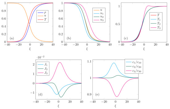
Figure 1.
Shock structure for , , , and : (a) mixture field variables; (b) velocities; (c) temperatures; (d) diffusion fluxes; (e) concentrations.
Case 2. In the second case, two profiles were computed for the same value of Mach number, . The difference appears in equilibrium concentrations: for , , and , profiles are presented in Figure 2, graphs (a) and (b); for , , and , profiles are presented in Figure 2, graphs (c) and (d). The profiles consist of two zones: upstream one with steeper gradients of field variables, and downstream one with moderate gradients. This appears to be more prominent in the profiles of mixture variables, especially on graph (a). This kind of profile, named Type-C, was firstly observed in [59] for the shock structure in ET14 model of a polyatomic gas (see also [18] for a contextualized account). The result was further supported by numerical solution of the Boltzmann equation for polyatomic gases [60], as well as two-temperature Navier–Stokes equations for polyatomic gases [61]. The main cause of such a profile is attributed to the presence of dynamic pressure and its relaxation (bulk viscosity), which is longer than the relaxation of viscous stress and heat flux. Although our model does not take into account these processes, there exists certain resemblance to this phenomenon in our profiles as well. To the best of our knowledge, such profiles do not appear in monatomic gases and their mixtures, and we are convinced that polyatomic molecular structure is the cause for this result. Note that such profiles appear in the case with an overshoot and without it alike.
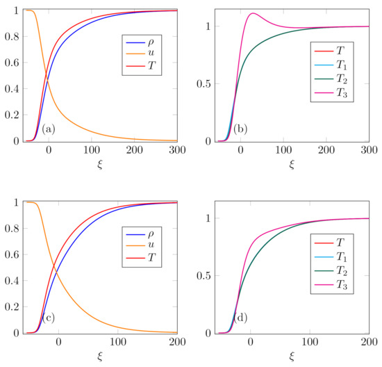
Figure 2.
Shock structure for , , , and : (a) mixture field variables; (b) temperatures. Shock structure for , , , and : (c) mixture field variables; (d) temperatures.
Case 3. In this case we examined the profiles with the highest equilibrium concentration . In particular, we computed the profiles for , and , and for two different values of Mach number, and , presented in Figure 3a,b, respectively. For these profiles it is remarkable that temperatures of the constituents have negligibly small difference, which is almost indistinguishable on the scale of graph (and thus not presented here). Therefore, we present the two cases which are in accordance with the results for binary mixture [47]—shock thickness decreases with the increase of Mach number. This conclusion is valid for small values of .
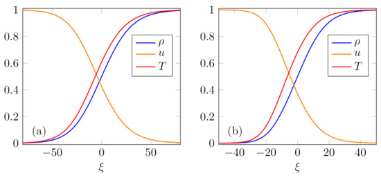
Figure 3.
Shock structure for , and : (a) mixture field variables for ; (b) mixture field variables for .
Case 4. Here we computed the profiles for , and . However, we analyzed two different cases: (a) and , and (b) and , presented in Figure 4. These results give an insight into the influence of mass ratio on the shock structure. In case (a), in the mixture with disparate masses of constituents, one may observe the temperature overshoot in . However, in case (b) where constituents 2 and 3 have comparable masses, temperatures of the constituents are almost indistinguishable.
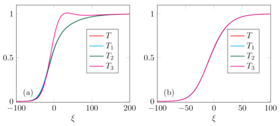
Figure 4.
Shock structure for , and : (a) temperatures for and ; (b) temperatures for and .
4.2. Comparison with a Single-Temperature Model
There always appears a question of the relevance of the MT assumption in the mixtures. Certainly, there are non-equilibrium processes in which this assumption cannot be dropped (e.g., in plasma). On the other hand, it also proved to be relevant in mixtures whose constituents have disparate atomic/molecular masses, like noble gases. Within the framework of RET, even if the multi-temperature assumption is dropped, one ends up with a multi-velocity model which is still hyperbolic and does not produce the paradox of infinite speed of pulse propagation.
Our intention is to quantify the discrepancy in mixture field variables, primarily in the average temperature of the mixture, which appears within the shock profile computed for MT model, and the one computed for ST model. To that end, we compute the sup-norm of the difference of numerically computed solutions, i.e., , where denotes the temperature field along the shock profile in ST model.
For the shock structure with a temperature overshoot, presented in Case 1. of this study, sup-norm of the difference of normalized temperature profiles (the ones whose equilibrium values are set to and ) is (see Figure 5). This implies that processes of energy exchange between the constituents, which appear due to the temperature difference, do not have a significant influence on the average value of temperature in MT model. However, this does not mean that they may be neglected. It was shown that appearance of temperature overshoot is directly related to insufficient energy exchange/transfer [43,47]. Additionally, preliminary computations, not reported here, show that there are cases with extremely large temperature overshoot, , in which ST is not capable of proper capturing the behavior of the mixture temperature. This will be the subject of our prospective study.
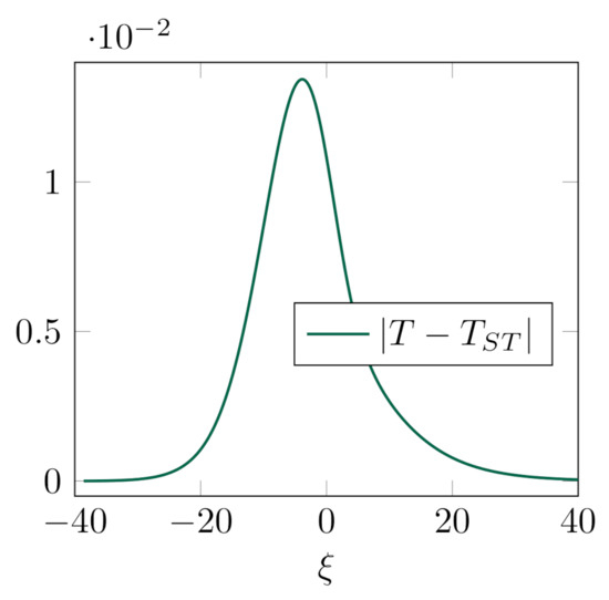
Figure 5.
Difference of the mean temperatures in MT and ST model, computed for the Case 1, , , , and .
5. Relaxation in the Shock Structure
One of the main features of hyperbolic systems of balance laws is that dissipation is achieved through the relaxation process, i.e., convergence of non-equilibrium variables to a certain (local) equilibrium state. Quantitative measure of the rate of convergence towards equilibrium is relaxation time. In simpler mathematical models, relaxation time may be unique for the whole system. However, if the model describes complex physical processes, there may be a need for more than one relaxation time. This is the case in our model of multi-component mixtures.
Mechanical (diffusion) and thermal relaxation times were introduced in (25), while their influence on the source terms was described in (26). It was shown recently [53] that the rate of convergence may not be the same for different processes. Therefore, our aim is to compare different relaxation times and to get an insight to the rate of convergence towards equilibrium for different processes. We shall compare the relaxation times in a relative sense, i.e., by computing the ratio of relaxation times and to the reference relaxation time along the shock profiles. After straightforward calculation, one may find the explicit dimensionless form of ratios of the diffusion relaxation times to the reference one:
Ratios of the thermal relaxation times to the reference one in dimensionless form read:
Ratios of the phenomenological coefficients needed to complete these expressions are given in the Appendix A.
Relaxation times, presented in Figure 6, are computed for the profiles analyzed in Case 1. They share one common property—a decrease along the shock profile, although it may not be monotonic. However, the most remarkable feature of the relaxation times in the multi-component mixture, at least in this case, is that the thermal relaxation times are considerably smaller than the diffusion relaxation times . These results oppose the ones obtained in the case of binary mixture [40,47], even when the viscous and thermal dissipation are taken into account [53]. This certainly calls for deeper analysis of relaxation processes in the mixture. Additionally, it must be kept in mind that relaxation times may be strictly related to the rate of convergence towards equilibrium only in the simplest possible space-homogeneous cases. Therefore, relaxation times (25) in our model cannot be simply identified as the time-rates of convergence of non-equilibrium variables.
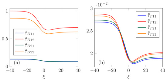
Figure 6.
Relaxation times in the shock structure for , , , and : (a) mechanical (diffusion) relaxation times; (b) thermal relaxation times.
6. Conclusions and Outlook
This paper was devoted to the study of shock structure in multi-component mixture of Euler fluids. Analysis was based upon the hyperbolic MT model for mixtures developed within the framework of RET. Explicit form of phenomenological coefficients, which appear in the source terms, was determined by matching with a linearized weak form of the collision operator in the system of Boltzmann equations for mixtures of polyatomic gases. The analysis was restricted to the normal shock waves, smeared out into a shock structure due to dissipation. Therefore, the shock structure was assumed in the form of a traveling wave. The original governing equations are transformed into a system of ODE’s that determine the shock structure as a heteroclinic orbit which asymptotically connects stationary points. Shock profiles were found as numerical solutions to the system of shock structure equations in dimensionless form, and analyzed for the several different sets of values of the parameters.
Our attention was focused on cases which possess certain distinguishing features, and thus can be taken as representatives of a broader class of qualitatively similar shock profiles. In particular, the following representative cases were recognized:
- (a)
- shock profiles with an overshoot in (the temperature of the heaviest constituent); this appears in the mixture with disparate masses of the constituents, , , and when the equilibrium concentration of the heaviest constituent is small;
- (b)
- shock profiles with two zones; in this case one distinguishes the front part of the profile, with steep gradients of field variables, and the rear part with moderate gradients of field variables;
- (c)
- shock profiles with small magnitude of the diffusion temperatures, and decreasing thickness with the increase of Mach number; this case is typical for large equilibrium concentration of the heaviest constituent;
- (d)
- shock profiles which depend on the mass ratio; increase of the mass ratio leads to disappearance of the temperature overshoot, and resembles the behavior of binary mixture.
We also analyzed the ST model and compared its profiles with the MT ones. It was recognized that MT assumption does not produce significant difference between the profiles of the average temperatures in MT and ST case. However, certain profiles exist with larger magnitude of temperature overshoot, and systematic analysis of MT assumption in these cases is a matter of ongoing research.
Finally, to perceive the rate at which dissipation occurs, we computed the relaxation times which appear in the source terms. It was found out that relaxation times decreased along the shock profile (but not monotonically). Analysis also shed new light on their magnitudes by giving an estimate that thermal relaxation times could be smaller than the diffusion ones.
The present study opens a new chapter in analysis of the shock structure in gaseous mixtures. It is important to note that the model took advantage of the continuum approach, which secured thermodynamic consistency and peculiar structure of the source terms, and the kinetic theory, which equipped us with explicit form of the phenomenological coefficients. In such a way we obtain reliable and tractable mathematical model at the same time. Results obtained in this way are in good agreement with the results of other studies, and therefore confirm validity of the model. Further analysis, which is a work in progress, will be concerned with a systematic study of the shock structure in the regions of parameter space in which continuous solutions exist. This will give a deeper insight into the influence of certain parameters on quantitative characteristics of the shock profiles, like the temperature overshoot or the shock thickness. Additionally, in continuation, it is our intention to extend the analysis of the entropy growth and the entropy production rate, given in [52] for the binary mixture, to three-component mixtures. Our aim is also to take into account viscous and thermal dissipation and evaluate their influence on the shock structure in multi-component mixtures, like it was done in [53] for binary mixtures. Finally, it is our intent to analyze the cases of specific mixtures. To that end we plan to use novel models of polyatomic gases, derived in the kinetic theory [21], to get better estimates of phenomenological coefficients and to relate them to measurable physical quantities like diffusivity. This will also lead to possible explicit estimate of the shock thickness in terms of the average mean free path of the molecules.
Author Contributions
Conceptualization, M.P.-Č. and S.S.; methodology, D.M., M.P.-Č. and S.S.; software, D.M.; formal analysis, M.P.-Č. and S.S.; investigation, D.M. and M.P.-Č.; writing—original draft preparation, M.P.-Č. and S.S.; writing—review and editing, D.M., M.P.-Č. and S.S.; visualization, D.M.; funding acquisition, M.P.-Č. and S.S. All authors have read and agreed to the published version of the manuscript.
Funding
This research was funded (D. Madjarević and M. Pavić-Čolić) by the support of the Program for Excellent Projects of Young Researchers (PROMIS) of the Science Fund of the Republic of Serbia as members of the project MaKiPol #6066089, Mathematical methods in the kinetic theory of polyatomic gas mixtures: modelling, analysis and computation, whose support enabled publication of this article in an open access manner. The research was also supported (S. Simić) by the Ministry of Education, Science and Technological Development of the Republic of Serbia (Grant No. 451-03-9/2021-14/ 200125).
Conflicts of Interest
The authors declare no conflict of interest.
Abbreviations
| RET | Rational extended thermodynamics |
| MT | Multi-temperature |
| ST | Single-temperature |
Appendix A
Here we list the ratios of phenomenological coefficients which appear in the dimensionless form of the source terms (37) and (38). We use the abbreviated notation, , , and denotes the phenomenological coefficient evaluated at upstream equilibrium. We also take into account that coefficients are symmetric, i.e., and .
Ratios of coefficients in (37) read:
Ratios of coefficients in (38) read:
Ratios of coefficients given above are expressed in terms of given in (22). Taking into account (22)–(24), one may find their explicit form:
To facilitate numerical computation, we list below some useful expressions which appear in the model:
References
- Courant, R.; Friedrichs, K.O. Supersonic Flow and Shock Waves; Springer: New York, NY, USA, 1976; Volume 21. [Google Scholar]
- Zel’dovich, Y.B.; Raizer, Y.P. Physics of Shock Waves and High-Temperature Hydrodynamic Phenomena; Dover Publications Inc.: New York, NY, USA, 2002. [Google Scholar]
- Lax, P. Shock waves and entropy. In Contributions to Nonlinear Functional Analysis; Academic Press: Cambridge, MA, USA, 1971; pp. 603–634. [Google Scholar]
- Dafermos, C. Hyperbolic Conservation Laws in Continuum Physics; Springer: Berlin/Heidelberg, Germany, 2016. [Google Scholar]
- Liu, I.-S. Continuum Mechanics; Springer: Berlin/Heidelberg, Germany, 2002. [Google Scholar]
- Müller, I. Thermodynamics; Pitman: London, UK, 1985. [Google Scholar]
- Chen, G.-Q.; Levermore, C.D.; Liu, T.-P. Hyperbolic conservation laws with stiff relaxation terms and entropy. Commun. Pure Appl. Math. 1994, 47, 787–830. [Google Scholar] [CrossRef]
- Ikenberry, E.; Turesdell, C. On the Pressures and the Flux of Energy in a Gas according to Maxwell’s Kinetic Theory, I. J. Ration. Mech. Anal. 1956, 5, 1–54. [Google Scholar] [CrossRef][Green Version]
- Yang, Z.; Yong, W.-A. Validity of the Chapman–Enskog expansion for a class of hyperbolic relaxation systems. J. Differ. Equ. 2015, 258, 2745–2766. [Google Scholar] [CrossRef]
- Ruggeri, T. Can constitutive relations be represented by non-local equations? Q. Appl. Math. 2012, 70, 597–611. [Google Scholar] [CrossRef]
- Kogan, M.N. Rarefied Gas Dynamics; Plenum Press: New York, NY, USA, 1969. [Google Scholar]
- Grad, H. On the kinetic theory of rarefied gases. Commun. Pure Appl. Math. 1949, 2, 331–407. [Google Scholar] [CrossRef]
- Müller, I.; Ruggeri, T. Rational Extended Thermodynamics; Springer: New York, NY, USA, 1998. [Google Scholar]
- Boudin, L.; Grec, B.; Salvarani, F. A mathematical and numerical analysis of the Maxwell-Stefan diffusion equations. Discret. Contin. Dyn. Syst. Ser. B 2012, 17, 1427–1440. [Google Scholar] [CrossRef]
- Boudin, L.; Grec, B.; Pavan, V. The Maxwell-Stefan diffusion limit for a kinetic model of mixtures with general cross sections. Nonlinear Anal. 2017, 159, 40–61. [Google Scholar] [CrossRef][Green Version]
- Salvarani, F.; Soares, A.J. On the relaxation of the Maxwell-Stefan system to linear diffusion. Appl. Math. Lett. 2018, 85, 15–21. [Google Scholar] [CrossRef]
- Ruggeri, T.; Simić, S. On the hyperbolic system of a mixture of Eulerian fluids: A comparison between single-and multi-temperature models. Math. Methods Appl. Sci. 2007, 30, 827–849. [Google Scholar] [CrossRef]
- Ruggeri, T.; Sugiyama, M. Rational Extended Thermodynamics Beyond the Monatomic Gas; Springer: New York, NY, USA, 2015. [Google Scholar]
- Bourgat, J.-F.; Desvillettes, L.; Le Tallec, P.; Perthame, B. Microreversible collisions for polyatomic gases. Eur. J. Mech. B/Fluids 1994, 13, 237–254. [Google Scholar]
- Desvillettes, L.; Monaco, R.; Salvarani, F. A kinetic model allowing to obtain the energy law of polytropic gases in the presence of chemical reactions. Eur. J. Mech. B/Fluids 2005, 24, 219–236. [Google Scholar] [CrossRef]
- Djordjić, V.; Pavić-Čolić, M.; Spasojević, N. Polytropic gas modelling at kinetic and macroscopic levels. Kinet. Relat. Models 2021. [Google Scholar] [CrossRef]
- Dellacherie, S. On the Wang Chang-Uhlenbeck equations. Discret. Contin. Dyn. Syst. Ser. B 2003, 3, 229–253. [Google Scholar]
- Giovangigli, V. Multicomponent Flow Modeling; Birkhäuser: Boston, MA, USA, 1999. [Google Scholar]
- Nagnibeda, E.; Kustova, E. Non-Equilibrium Reacting Gas Flows: Kinetic Theory of Transport and Relaxation Processes; Springer: Berlin/Heidelberg, Germany, 2009. [Google Scholar]
- Kremer, G.M. An Introduction to the Boltzmann Equation and Transport Processes in Gases; Springer: Berlin/Heidelberg, Germany, 2010. [Google Scholar]
- Pavić, M.; Ruggeri, T.; Simić, S. Maximum entropy principle for rarefied polyatomic gases. Phys. A Stat. Mech. Appl. 2013, 392, 1302–1317. [Google Scholar] [CrossRef]
- Pavić-Čolić, M.; Simić, S. Moment equations for polyatomic gases. Acta Appl. Math. 2014, 132, 469–482. [Google Scholar] [CrossRef]
- Baranger, C.; Bisi, M.; Brull, S.; Desvillettes, L. On the Chapman-Enskog asymptotics for a mixture of monoatomic and polyatomic rarefied gases. Kinet. Relat. Models 2018, 11, 821–858. [Google Scholar] [CrossRef]
- Anwasia, B.; Bisi, M.; Salvarani, F.; Soares, A.J. On the Maxwell-Stefan diffusion limit for a reactive mixture of polyatomic gases in non-isothermal setting (English summary). Kinet. Relat. Models 2020, 13, 63–95. [Google Scholar] [CrossRef]
- Gamba, I.M.; Pavić-Čolić, M. On the Cauchy problem for Boltzmann equation modelling a polyatomic gas. arXiv 2020, arXiv:2005.01017. [Google Scholar]
- Bisi, M.; Martalò, G.; Spiga, G. Multi-temperature Euler hydrodynamics for a reacting gas from a kinetic approach to rarefied mixtures with resonant collisions. EPL (Europhys. Lett.) 2011, 95, 55002. [Google Scholar] [CrossRef]
- Bisi, M.; Groppi, M.; Martalò, G. Macroscopic equations for inert gas mixtures in different hydrodynamic regimes. J. Phys. A Math. Theor. 2021, 54, 085201. [Google Scholar] [CrossRef]
- Pavić-Čolić, M. Multi-velocity and multi-temperature model of the mixture of polyatomic gases issuing from kinetic theory. Phys. Lett. A 2019, 383, 2829–2835. [Google Scholar] [CrossRef]
- Gilbarg, D.; Paolucci, D. The structure of shock waves in the continuum theory of fluids. J. Ration. Mech. Anal. 1953, 2, 617–642. [Google Scholar] [CrossRef]
- Weiss, W. Continuous shock structure in extended thermodynamics. Phys. Rev. E 1995, 52, R5760. [Google Scholar] [CrossRef] [PubMed]
- Achleitner, F.; Szmolyan, P. Saddle–node bifurcation of viscous profiles. Phys. D Nonlinear Phenom. 2012, 241, 1703–1717. [Google Scholar] [CrossRef] [PubMed][Green Version]
- Simić, S. Shock structure in continuum models of gas dynamics: Stability and bifurcation analysis. Nonlinearity 2009, 22, 1337. [Google Scholar] [CrossRef]
- Boillat, G.; Ruggeri, T. On the shock structure problem for hyperbolic system of balance laws and convex entropy. Contin. Mech. Thermodyn. 1998, 10, 285–292. [Google Scholar] [CrossRef]
- Sherman, F.S. Shock-wave structure in binary mixtures of chemically inert perfect gases. J. Fluid Mech. 1960, 8, 465–480. [Google Scholar] [CrossRef]
- Bird, G. The structure of normal shock waves in a binary gas mixture. J. Fluid Mech. 1968, 31, 657–668. [Google Scholar] [CrossRef]
- Kosuge, S.; Aoki, K.; Takata, S. Shock-wave structure for a binary gas mixture: Finite-difference analysis of the Boltzmann equation for hard sphere molecules. Eur. J. Mech. B/Fluids 2001, 20, 87–126. [Google Scholar] [CrossRef]
- Raines, A.A. Study of a shock wave structure in gas mixtures on the basis of the Boltzmann equation. Eur. J. Mech. B/Fluids 2002, 21, 599–610. [Google Scholar] [CrossRef]
- Abe, K.; Oguchi, H. Shock wave structures in binary gas mixtures with regard to temperature overshoot. Phys. Fluids 1974, 17, 1333–1334. [Google Scholar] [CrossRef]
- Bisi, M.; Martalò, G.; Spiga, G. Shock wave structure of multi-temperature Euler equations from kinetic theory for a binary mixture. Acta Appl. Math. 2014, 132, 95–105. [Google Scholar] [CrossRef][Green Version]
- Bisi, M.; Groppi, M.; Martalò, G. On the shock thickness for a binary gas mixture. Ric. Mat. 2020, in press. [Google Scholar] [CrossRef]
- Madjarević, D.; Simić, S. Shock structure in helium-argon mixture—A comparison of hyperbolic multi-temperature model with experiment. EPL (Europhys. Lett.) 2013, 102, 44002. [Google Scholar] [CrossRef]
- Madjarević, D.; Ruggeri, T.; Simić, S. Shock structure and temperature overshoot in macroscopic multi-temperature model of mixtures. Phys. Fluids 2014, 26, 106102. [Google Scholar] [CrossRef]
- Conforto, F.; Mentrelli, A.; Ruggeri, T. Shock structure and multiple sub-shocks in binary mixtures of Eulerian fluids. Ric. Mat. 2017, 66, 221–231. [Google Scholar] [CrossRef]
- Artale, V.; Conforto, F.; Martalò, G.; Ricciardello, A. Shock structure and multiple sub-shocks in Grad 10-moment binary mixtures of monoatomic gases. Ric. Mat. 2019, 68, 485–502. [Google Scholar] [CrossRef]
- Bisi, M.; Groppi, M.; Macaluso, A.; Martalò, G. Shock wave structure of multi-temperature Grad 10-moment equations for a binary gas mixture. EPL (Europhys. Lett.) 2021, 133, 54001. [Google Scholar] [CrossRef]
- Sharipov, F.; Dias, F.C. Structure of planar shock waves in gaseous mixtures based on ab initio direct simulation. Eur. J. Mech. B/Fluids 2018, 72, 251–263. [Google Scholar] [CrossRef]
- Madjarević, D.; Simić, S. Entropy growth and entropy production rate in binary mixture shock waves. Phys. Rev. E 2019, 100, s023119. [Google Scholar] [CrossRef] [PubMed]
- Simić, S.; Madjarević, D. Shock structure and entropy growth in a gaseous binary mixture with viscous and thermal dissipation. Wave Motion 2021, 100, 102661. [Google Scholar] [CrossRef]
- Ruyev, G.A.; Fedorov, A.V.; Fomin, V.M. Special features of the shock-wave structure in mixtures of gases with disparate molecular masses. J. Appl. Mech. Tech. Phys. 2002, 43, 529–537. [Google Scholar] [CrossRef]
- Josyula, E.; Vedula, P.; Bailey, W.F.; Suchyta, C.J., III. Kinetic solution of the structure of a shock wave in a nonreactive gas mixture. Phys. Fluids 2011, 23, 017101. [Google Scholar] [CrossRef]
- Raines, A.A. Numerical solution of the Boltzmann equation for the shock wave in a gas mixture. arXiv 2014, arXiv:1403.3230. [Google Scholar]
- Truesdell, C. Rational Thermodynamics; Springer: New York, NY, USA, 1984. [Google Scholar]
- Boillat, G.; Ruggeri, T. Hyperbolic principal subsystems: Entropy convexity and subcharacteristic conditions. Arch. Ration. Mech. Anal. 1997, 137, 305–320. [Google Scholar] [CrossRef]
- Taniguchi, S.; Arima, T.; Ruggeri, T.; Sugiyama, M. Effect of the dynamic pressure on the shock wave structure in a rarefied polyatomic gas. Phys. Fluids 2014, 26, 016103. [Google Scholar] [CrossRef]
- Kosuge, S.; Aoki, K. Shock-wave structure for a polyatomic gas with large bulk viscosity. Phys. Rev. Fluids 2018, 3, 023401. [Google Scholar] [CrossRef]
- Aoki, K.; Bisi, M.; Groppi, M.; Kosuge, S. Two-temperature Navier-Stokes equations for a polyatomic gas derived from kinetic theory. Phys. Rev. E 2020, 102, 023104. [Google Scholar] [CrossRef] [PubMed]


Publisher’s Note: MDPI stays neutral with regard to jurisdictional claims in published maps and institutional affiliations. |
© 2021 by the authors. Licensee MDPI, Basel, Switzerland. This article is an open access article distributed under the terms and conditions of the Creative Commons Attribution (CC BY) license (https://creativecommons.org/licenses/by/4.0/).