Reversible Data Hiding in Encrypted Images Using Median Edge Detector and Two’s Complement

Abstract

With the rapid development of cloud storage, an increasing number of users store their images in the cloud. These images contain many business secrets or personal information, such as engineering design drawings and commercial contracts. Thus, users encrypt images before they are uploaded. However, cloud servers have to hide secret data in encrypted images to enable the retrieval and verification of massive encrypted images. To ensure that both the secret data and the original images can be extracted and recovered losslessly, researchers have proposed a method that is known as reversible data hiding in encrypted images (RDHEI). In this paper, a new RDHEI method using median edge detector (MED) and two’s complement is proposed. The MED prediction method is used to generate the predicted values of the original pixels and calculate the prediction errors. The adaptive-length two’s complement is used to encode the most prediction errors. To reserve room, the two’s complement is labeled in the pixels. To record the unlabeled pixels, a label map is generated and embedded into the image. After the image has been encrypted, it can be embedded with the data. The experimental results indicate that the proposed method can reach an average embedding rate of 2.58 bpp, 3.04 bpp, and 2.94 bpp on the three datasets, i.e., UCID, BOSSbase, BOWS-2, which outperforms the previous work.

1. Introduction

Data-hiding technology [1] plays a significant role in image fields such as identification, annotation, and copyright. However, the traditional data-hiding method [2] causes permanent distortion of the original images. In the judicial, medical, and military fields, each bit of an image is essential, and any distortion in images is unacceptable. This has led to an interest in the reversible data-hiding (RDH) method. RDH methods [3,4,5] can hide data and achieve the lossless recovery of the original images. However, the early RDH methods could not achieve a good performance. In the past decade, some effective RDH methods have been designed to achieve a better embedding rate and can be divided into three fundamental categories: lossless compression [6,7,8], difference expansion [9,10,11], and histogram shifting [12,13,14]. Combining the advantages of the above three different methods, researchers have proposed the combined strategies [15,16,17].

At present, cloud storage has become a popular service, especially for images, which need large storage space [18]. In the cloud scenario, RDH is an important method for cloud servers to manage outsourced images [19,20]. However, some cloud servers cannot be trusted, and storing images on the cloud may lead to privacy leakage [21]. To protect privacy, users encrypt their images before uploading them. Thus, it is vital to enable the cloud server to efficiently manage the encrypted images and allow the user to recover the original image losslessly at the same time [22]. Under such demands, the method of reversible data hiding in encrypted images (RDHEI) attracts considerable interest from researchers.

The RDHEI method can achieve data hiding in encrypted images and lossless recovery of original images. Generally, three parties are involved in the RDHEI method: the content owner, the data hider, and the receiver [23]. For example, the cloud scenario is described as follows to explain the three parties in detail. As a content owner, the user stores a large number of encrypted images on remote cloud services. Meanwhile, the cloud server is the data hider. To manage the encrypted images, the cloud server must embed secret data into the images, such as authentication and content annotation [22]. The receiver can be the cloud server, the user, or the authorized third party. Based on the encrypted image with embedded data, the cloud server can extract authentication and content annotation, and the user can recover the original image.

In the past decade, researchers have proposed many effective RDHEI methods [24,25,26,27,28,29]. According to the different order, either before or after encryption, there are two kinds of categories in recent RDHEI methods: (1) the methods by vacating room after encryption (VRAE) [24,25,26] and (2) the methods by reserving room before encryption (RRBE) [27,28,29]. In VRAE methods, the data hider vacates room on encrypted images. However, due to the chaos of encrypted images, it is difficult to create room. Thus, the embedding rates (ERs) of VRAE methods are low. On the other hand, in RRBE methods, the content owner reserves room before image encryption, so the spatial correlation of the original image can be used. After encryption, the data hider can embed data into the room reserved by the content owner. Thus, RRBE methods can achieve a higher embedding rate, and they have received increasing attention in recent years.

The first RRBE method was proposed by Ma et al. [27] in 2013. The original image was divided into two parts, i.e., A and B. The least significant bits (LSBs) of A are embedded into B using an RDH method to reserve room. Thus, after the encryption of the image, the LSBs of A can be used to embed data. Based on [27], Mathew and Wilscy [28] proposed an improved method using active block exchange in 2014. They divided the original image into smooth blocks and active blocks, and then they rearranged all the blocks to obtain a smooth area and an active area. To reserve room, one or more LSB planes of the active area are embedded in the smooth area. In 2014, Zhang et al. [29] proposed a new RRBE method. They used sample pixels to predict other pixels, and then they used prediction errors to replace the predicted pixels. During the encryption process, only the sample pixels are encrypted. According to the histogram of the encrypted image, the data are embedded by shifting the prediction errors. The algorithms of the RRBE methods [27,28,29] use the traditional algorithms of the RDH methods, and the maximum ER is almost 0.5 bits per pixel (bpp).

In 2016, Puteaux et al. [30] introduced a novel RRBE method using the most significant bit (MSB) prediction. In their method, the data hider embeds the data by modifying the MSB plane of the encrypted image. In the recovery phase, due to the spatial correlation of the MSBs between adjacent pixels, a prediction can be made to recover the original MSBs. The maximum ER of the method proposed by Puteaux et al. [30] can be reached as high as 1 bpp. However, Puteaux et al. [30] modified the pixels for which the MSBs could not be predicted correctly. Thus, their method caused the irreversible distortion of the original image. To solve the distortion problem, in 2018, Puteaux and Puech [31] proposed an improved method that uses prediction error embedding. They divided the MSB plane into nonoverlapping blocks and set flag blocks to indicate the incorrect predicted MSB. In the data-embedding stage, the flag blocks do not embed data. Therefore, Puteaux and Puech’s method  [31] is completely reversible. Additionally, in 2018, Puyang et al. [32] extended Peteaux and Puech’s method [31] to two MSB planes, and the average ER of their method was 1.5 bpp. In 2019, Puteaux and Puech [33] improved their original method [31] by using other bit planes, and the average ER of the revised method was 2 bpp. In 2019, Chen and Chang [34] proposed a new method based on the bit plane compression. To reserve room, they compressed the front bit planes by extended run-length coding, and they obtained a higher average ER, i.e., 2.3 bpp. However, in [34], except for that on the MSB plane, the compression rate of bit planes was not high. Additionally, in 2019, Yin et al. [35] proposed a multi-MSB prediction and Huffman coding method. They compared the original pixel and predicted value from MSBs to LSBs and defined the length of the same bits as the pixel’s label. To reserve room, after the image was encrypted, they used Huffman coding to compress the labels and embedded the Huffman codes into the encrypted pixels. According to the Huffman code of each encrypted pixel, the data hider can embed data.

In 2019, based on prediction errors rather than MSB, Yi and Zhou [36] proposed a new RRBE method. First, they proposed a parametric binary tree labeling (PBTL) scheme. In the PBTL scheme, there are two selectable parameters $\alpha$ and $\beta$. Through the parameters and a binary tree, n binary codes of category $G_1$ and one binary code of category $G_2$ can be generated. Then, they divided the image into $s\times s$ non-overlapping blocks and defined the first pixel in each block as the reference pixel. They used the reference pixel to predict the remaining pixels in each block and calculated prediction errors between the predicted values and the original values. They coded the n-most distributed prediction errors with $G_1$ codes and coded the remaining prediction errors with $G_2$ code. After the image was encrypted, they labeled each pixel with the binary code of its prediction error. Finally, in each pixel labeled by the $G_1$ code, in addition to the bits occupied by the binary code, the remaining bits can be used to embed data. In method [36], the reference pixels in the prediction method occupy a certain proportion and cannot be utilized. Therefore, in 2019, Wu et al. [37] improved the method of [36] by using the median edge detector (MED) predictor, and they achieved an average ER as large as 2.5 bpp. 

The most published RDHEI methods [31,32,33,34,35,36,37] are designed for uncompressed images. Furthermore, some RDHEI methods that can be applied to compressed images, such as AMBTC-compressed images, are proposed. In 2018, Yin et al. [38] proposed an RDHEI method for AMBTC images. Additionally, in 2019, Shiu et al. [39] proposed an RRBE method combining interpolated AMBTC and Huffman coding to improve the ER.

Although the methods proposed in [36,37] achieved good improvements in the ER, these methods do not make full use of the prediction errors. In addition, in these methods, the content owner must share the auxiliary information with the data hider, such as the pixel labels or location map, thereby leaking the original image’s information to the data hider. Thus, to increase the ER and reduce the risk of sharing auxiliary information, a new RRBE method based on the prediction errors is proposed in this paper. The contributions of this paper are summarized as follows:

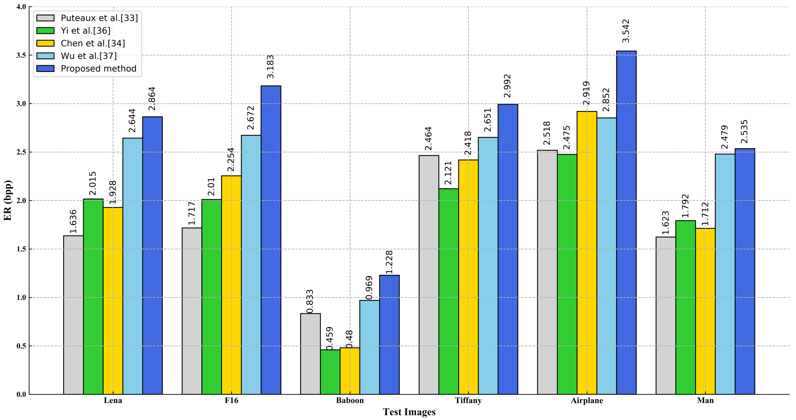
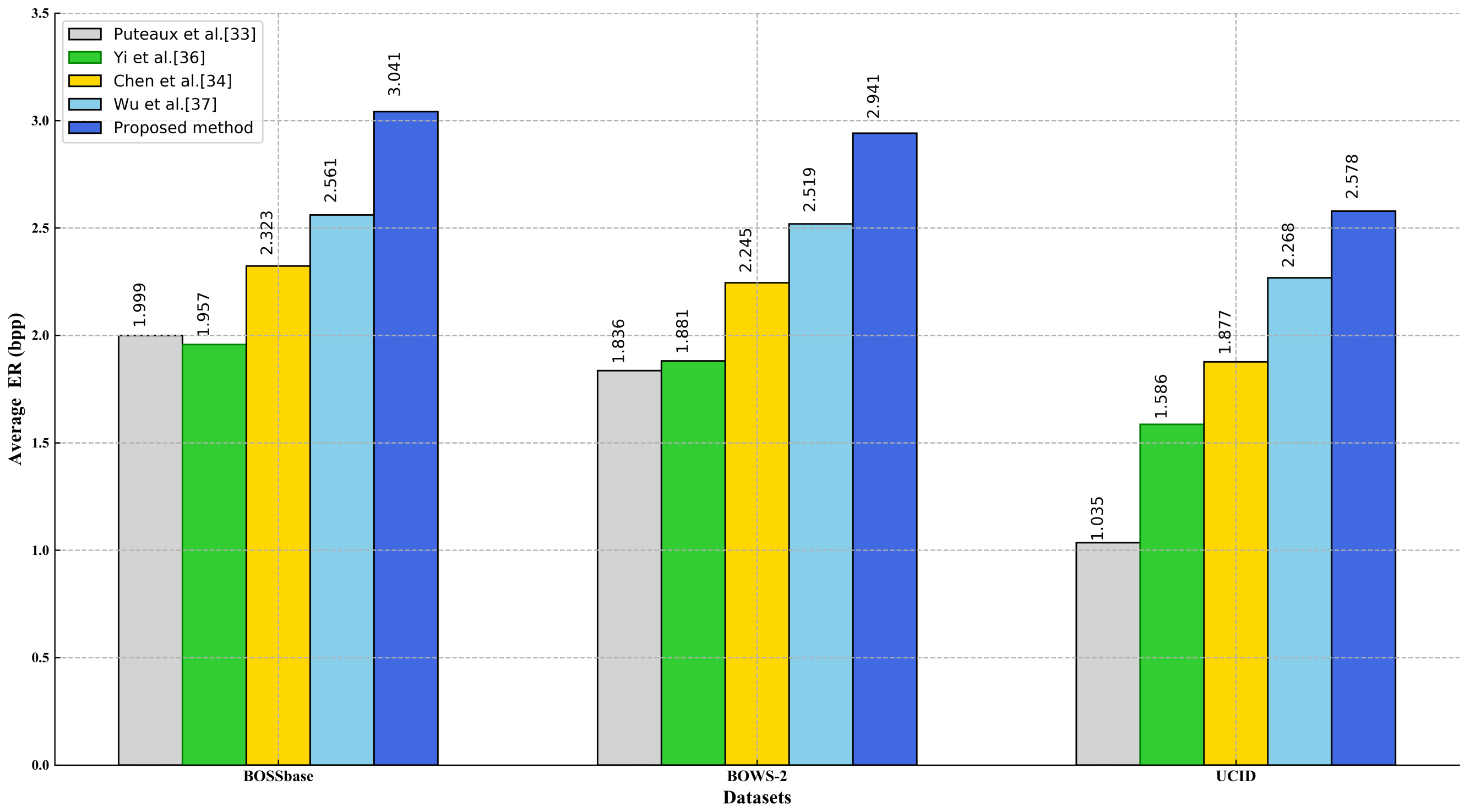
• The proposed method achieves a higher ER than previous related methods. In the proposed method, two’s complement is used to encode the prediction errors, making full use of spatial correlation. Therefore, more pixels are used to reserve room in the original image. Meanwhile, a label map is generated to record the overflowed pixels rather than embedding codes in these pixels. Compressing the label map can further reduce the room occupied by the auxiliary information. The experimental results show that the ERs of the proposed method are better than those of previous methods.
• The proposed method is more secure. In previous related methods, the auxiliary information is shared with the data hider for hiding data. Through the shared auxiliary information, a dishonest data hider can parse out the original image’s spatial information, which may cause leakage of the content. To solve this problem, an MSBs rearrangement method is proposed to form a regular reserved room. Then, the label map is embedded into the regular reserved room and encrypts. In addition, two parameters are set for hiding data, so the data hider cannot obtain any spatial information of the image. Thus, the proposed method reduces the risk of sharing auxiliary information.

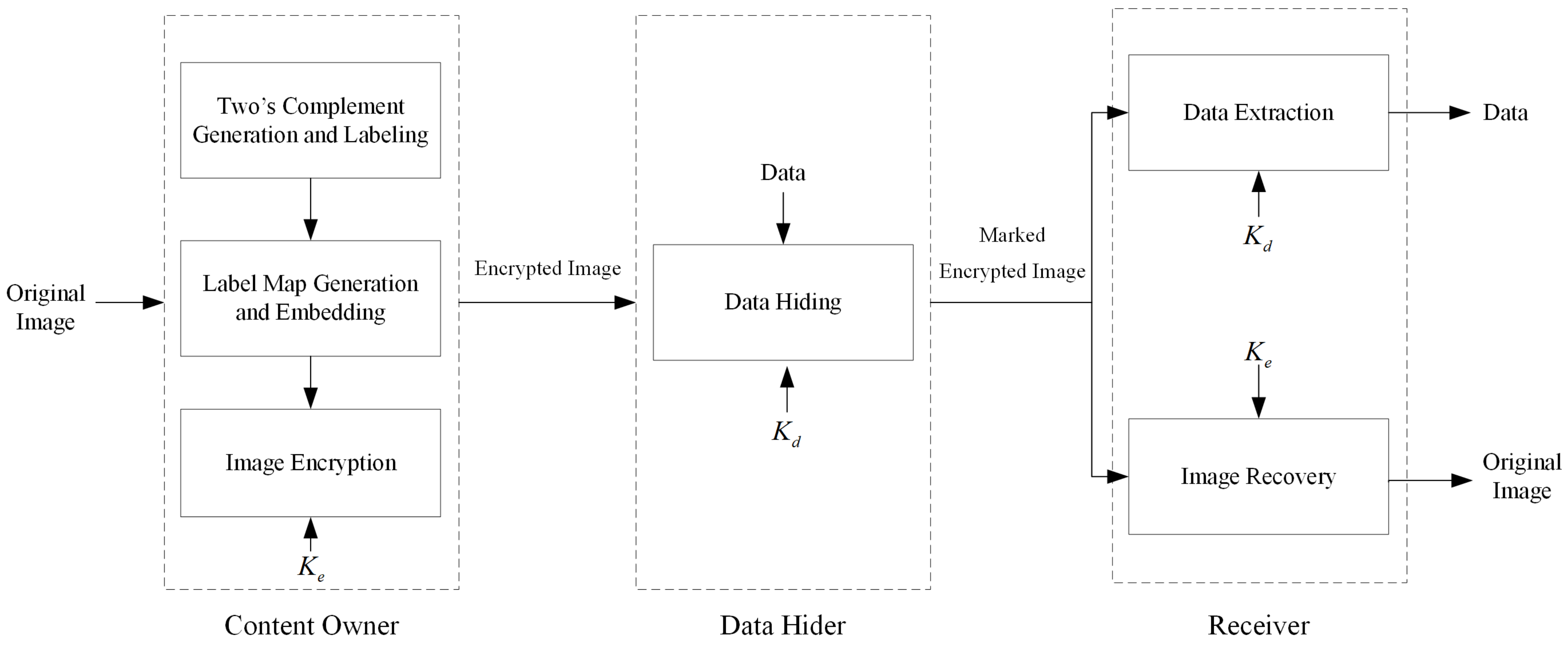
The rest of the paper is organized as follows. Section 2 describes the proposed RDHEI method. The experimental results are discussed in Section 3. Section 4 concludes this paper.

2. Proposed Method

This section describes the proposed method using the MED and two’s complement. There are three phases in our method: (1) the content owner processes the original image to reserve room and encrypts the image to protect the content; (2) the data hider embeds secret data in the encrypted image; (3) the receiver extracts the data and recovers the original images.

In the first phase, the content owner performs two’s complement generation and labeling methods in the original image to reserve room. Then, the content owner generates the label map as auxiliary information and embeds it in the image. Finally, the content owner encrypts the processed image using an encryption key $K_e$. In the second phase, after using a data hiding key $K_d$, the data hider embeds the secret data in the reserved room of the encrypted image. In the third phase, according to different keys, the receiver can extract the secret data or recover the original image losslessly from the marked encrypted image. An overview of the proposed method is shown in Figure 1. In addition, the main notations of this paper are listed in

Table 1. Summary of notations.

Notation	Meaning	Notation	Meaning
$I_o$	original image	$p_o(i,j)$	a pixel in $I_o$
$I_l$	labeled image	$p_l(i,j)$	a pixel in $I_l$
$I_p$	processed image	$p_p(i,j)$	a pixel in $I_p$
$I_e$	encrypted image	$p_e(i,j)$	a pixel in $I_e$
$I_m$	marked encrypted image	$p_m(i,j)$	a pixel in $I_m$
H	image height	W	image width
$v(i,j)$	predicted value of original pixel $p_o(i,j)$	$e(i,j)$	prediction error between $p_o(i,j)$ and $v(i,j)$
$K_e$	image encryption key	$K_d$	data hiding key
$\alpha$	length of two’s complement	U	encoded prediction errors’ interval
M	label map	$B_m$	bitstream of compressed M
$L_m$	length of $B_m$	$B_u$	bitstream of unlabeled pixels’ (8 − $\alpha$)-bit MSBs
$C_p$	last pixel’s coordinate of embedding area	$B_r$	original fix-length bitstream of the reference pixels
$L_1$	length of bits used for $\alpha$ and $C_p$	$L_2$	length of bits used for $L_m$

.

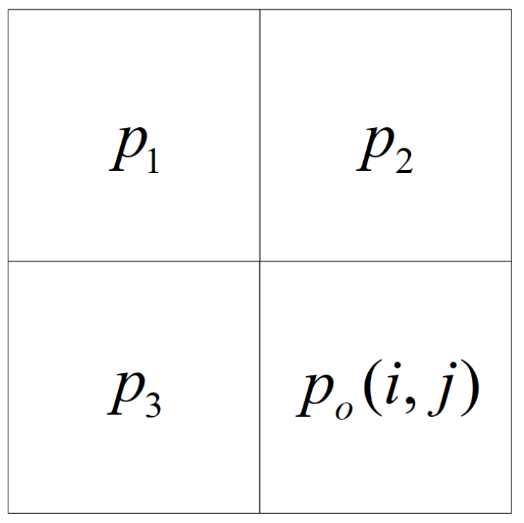
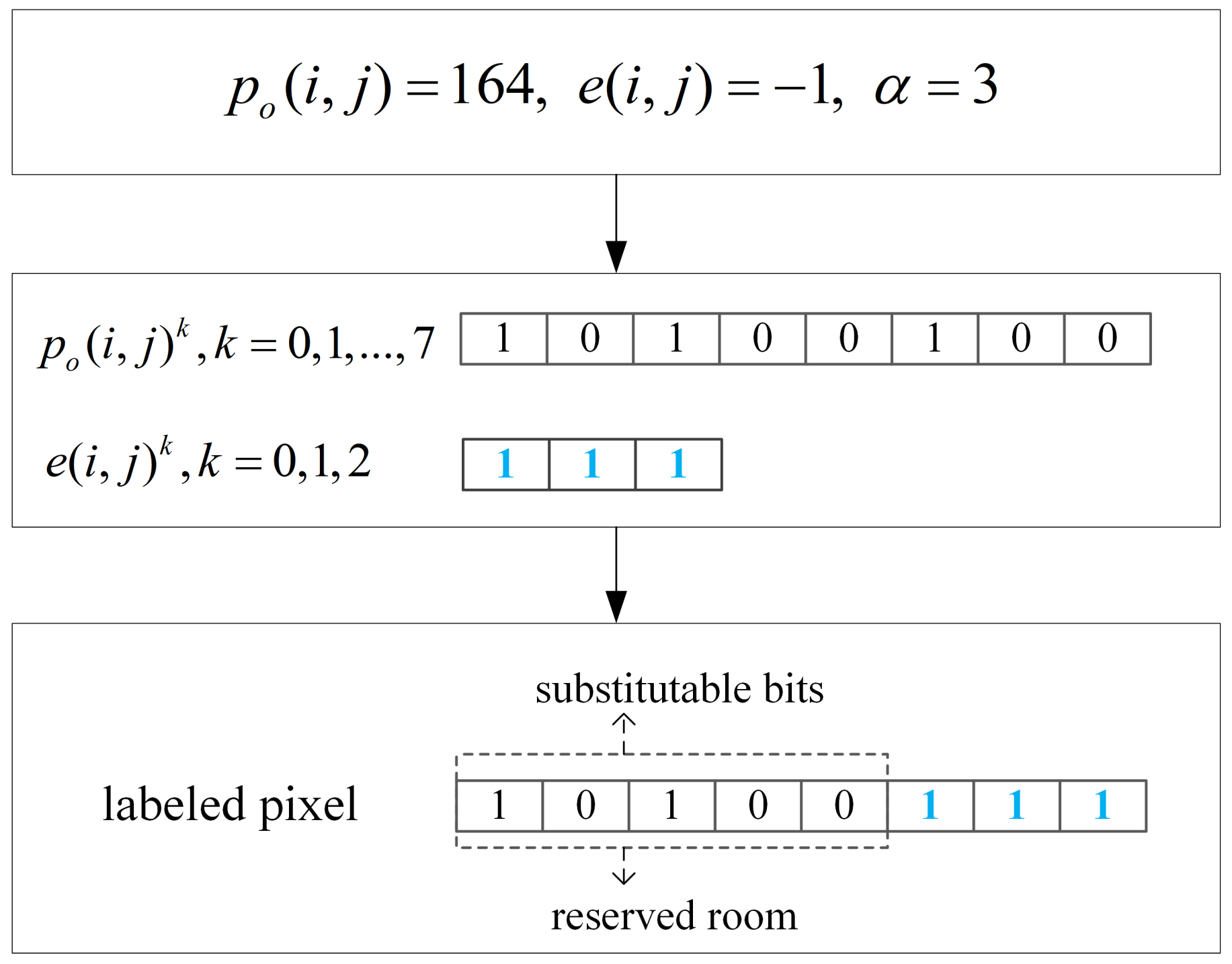
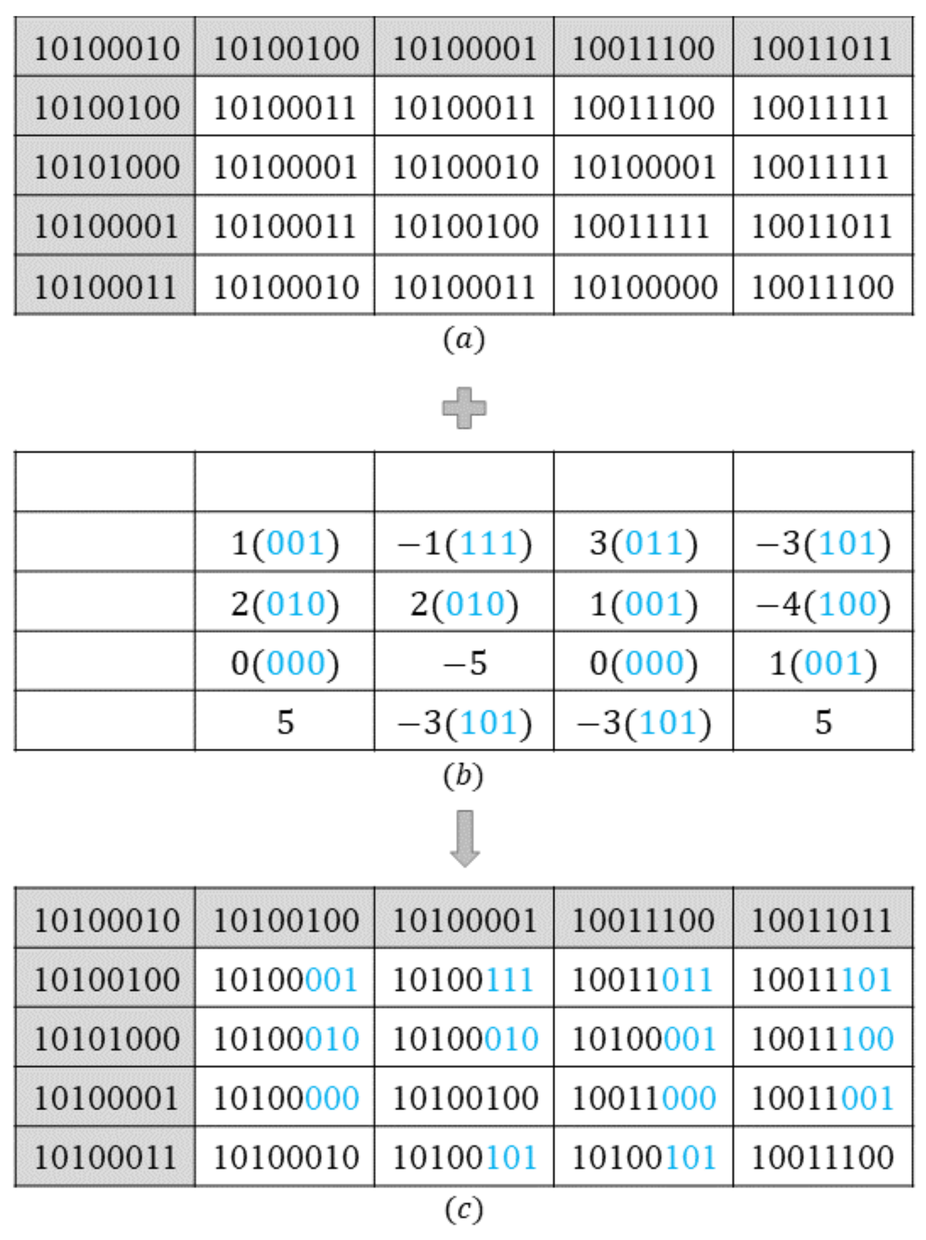
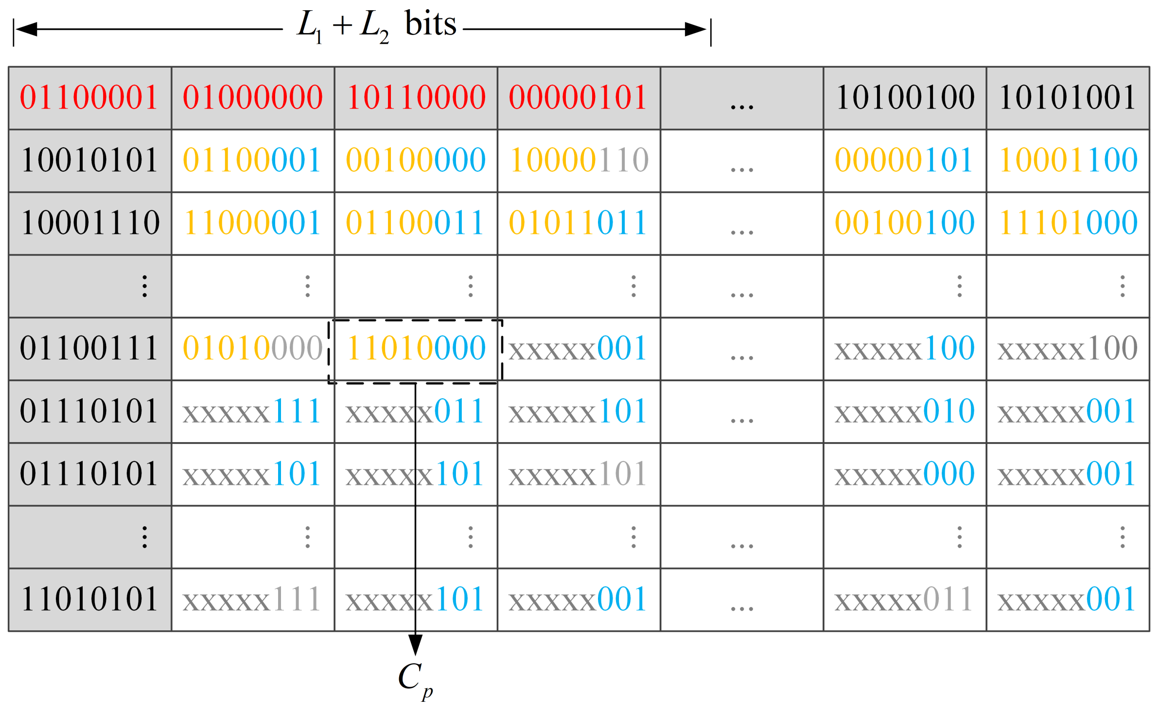
2.1. Two’s Complement Generation and Labeling

For an original image $I_o$ of size $H\times W$ with pixels $p_o(i,j)(1\le i\le H,1\le j\le W)$ in the range of $[0,255]$, a prediction process is done to generate the prediction errors. First, to obtain the predicted value of each original pixel, the MED prediction method is used. In the MED, the pixels in the first row and first column are recorded as reference pixels. In addition, a schematic diagram of MED is shown in Figure 2.

In Figure 2, $p_1$, $p_2$, and $p_3$ are three original pixels surrounding the currently predicted pixel $p_o(i,j)$. Then, the predicted value $v(i,j)$ of each remaining original pixel $p_o(i,j)(2\le i\le H,$$2\le j\le W)$ is calculated by the following formula:

$$v(i,j)=\left\{\begin{array}{cc}max(p_2,p_3),\hfill & p_1\le min(p_2,p_3)\hfill \\ min(p_2,p_3),\hfill & p_1\ge max(p_2,p_3)\hfill \\ p_2+p_3-p_1,\hfill & otherwise\hfill \end{array}\right.$$

Finally, each prediction error $e(i,j)$ between the original pixel $p_o(i,j)$ and the predicted value $v(i,j)$ is calculated by:

$$e(i,j)=p_o(i,j)-v(i,j)$$

Due to the spatial correlation of natural images, the distribution of prediction errors $e(i,j)(2\le i\le H,2\le j\le W)$ nearly follows a Laplace distribution with the location parameter equal to zero. Therefore, the center bins of the prediction errors distribution can record through two’s complement. Furthermore, two’s complement with different lengths can encode variable bins of prediction errors’ distribution.

For 8-bit depth pixels, it is assumed that the length of two’s complement is denoted $\alpha (1\le \alpha \le 7)$, the interval of the prediction errors that can be encoded by $\alpha$-bit two’s complement is $[-2^{\alpha -1},2^{\alpha -1}-1]$ (which is defined as U). Thus, an appropriate value of $\alpha$ can make the interval U contain the center bins of the distribution of the prediction errors. After determining $\alpha$, each pixel in $p_o(i,j)(2\le i\le H,2\le j\le W)$ can be divided into two categories according to its prediction error and U: (1) labeled pixel and (2) unlabeled pixel. The pixel that has a prediction error belongs to U is classified as the labeled pixel. Moreover, the pixel whose prediction error exceeds U is classified as the unlabeled pixel. The meaning of the label can be understood more in the following steps.

For the labeled pixels, their prediction errors can be encoded with $\alpha$-bit two’s complement. Based on this, a two’s complement labeling method is proposed to reserve room. First, converting each labeled pixel $p_o(i,j)$ into an 8-bit binary sequence. Each bit $p_o{(i,j)}^0,p_o{(i,j)}^1,\dots ,p_o{(i,j)}^7$ of the binary sequence can be calculated as:

$$p_o{(i,j)}^k=\lfloor \frac{p_o(i,j)}{2^k}\rfloor mod2,k=0,1,\dots ,7$$

where $\lfloor \rfloor$ is a floor function. Then, the prediction error $e(i,j)$ of the corresponding labeled pixel is encoded by the $\alpha$-bit two’s complement and each bit $e{(i,j)}^k(k=0,1,\dots ,\alpha -1)$ is calculated by:

$$e{(i,j)}^k=\left\{\begin{array}{cc}\lfloor \frac{e(i,j)}{2^k}\rfloor mod2,\hfill & e(i,j)\ge 0\hfill \\ \\ \lfloor \frac{2^{\alpha }+e(i,j)}{2^k}\rfloor mod2,\hfill & e(i,j)<0\hfill \end{array}\right.$$

Finally, in Figure 3, $e{(i,j)}^k(k=0,1,\dots ,\alpha -1)$ is embedded into $p_o{(i,j)}^k(k=0,1,\dots ,7)$ by LSB to ensure that the original pixel can be recovered. After embedding the predicted pixels’ prediction errors, the labeled pixels can be recovered by the $\alpha$-bit two’s complement. Therefore, the front (8 − $\alpha$)-bit MSBs of labeled pixels can be used to embed data.

On the other hand, for unlabeled pixels, their prediction errors cannot be encoded by $\alpha$-bit two’s complement. In other words, these pixels cannot be labeled with their prediction errors. The unlabeled pixels cannot be recovered after embedding the data. Thus, the unlabeled pixels must not be modified.

Through the two’s complement labeling method, a labeled image $I_l$ is generated. An example of the two’s complement labeling process on the part of Lena is shown in Figure 4, where $\alpha$ = 3. Figure 4a shows the binary sequences of the original pixels, and the gray blocks are reference pixels. Figure 4b shows the prediction errors of the original pixels, and the blue binary sequences are 3-bit two’s complement. Some prediction errors cannot be converted to 3-bit two’s complement because they are outside the interval $[-4,3]$, such as +5 and −5. The labeled image is shown in Figure 4c.

2.2. Label Map Generation and Embedding

The previous subsection describes different operations that are performed on each pixel based on its category (belonging to either labeled pixels or unlabeled pixels). However, as shown in Figure 4, the two’s complement of labeled pixels and the original bits of unlabeled pixels have the same situation. Thus, it is impossible to distinguish the category of each pixel by its LSB and to embed data in the labeled pixels. To identify each pixel’s category, a label map is used for the labeled image.

According to the principle of symmetry, a bitmap the same size as the labeled image is generated, which is defined as label map M. There is a symmetry relationship between the coordinates of M and $I_l$. Then, the values of M can be set through the pixel’s category of $I_l$. According to the coordinates of the labeled pixels, the values of the corresponding location in M are set to 0. On the other hand, the values corresponding to the unlabeled pixels in M are set to 1. Because of the spatial correlation of the images, the label map has a large number of 0 and a small number of 1. Based on this, the extended run-length coding method [34] is used to compress M losslessly, and the bitstream obtained after compression is defined as $B_m$.

After the compressed label map is obtained, $B_m$ must be embedded into the reserved room as auxiliary information. However, at the stage of image recovery, bitstream $B_m$ can be extracted when the pixels are divided into labeled or unlabeled. The identification information is derived from $B_m$. Thus, this is a paradox. To solve this problem, an MSBs rearrangement method is proposed to embed the label map. First, one extracts the (8 − $\alpha$)-bit MSBs of unlabeled pixels to generate a bitstream, $B_u$. Except for the reference pixels, the (8 − $\alpha$)-bit MSBs of each pixel in the labeled image is reserved room. Therefore, a regular reserved room is obtained. Then, to ensure that the unlabeled pixels can be recovered, bitstream $B_u$ is spliced to the tail of bitstream $B_m$ to obtain a new long bitstream. Thus, continuous pixels’ MSBs can be used to store the long bitstream regardless of whether the pixel is labeled or unlabeled. Finally, image $I_l$ is scanned from top to bottom and from left to right, and the long bitstream is embedded into the (8 − $\alpha$)-bit MSBs of each pixel by using bit substitution simultaneously. Note that the reference pixels are not used to embed the long bitstream. After the embedding of the long bitstream is completed, the last pixel’s coordinate of the embedding area is obtained. To extract the long bitstream from the image, the coordinate is stored and defined as parameter $C_p$, for example, $C_p=(123,45)$. To cut the long bitstream into $B_m$ and $B_u$, the length of $B_m$ is defined as parameter $L_m$, for example, $L_m=162,341$.

Additionally, for subsequent operation of data hiding and image recovery, the parameters $\alpha$, $C_p$, and $L_m$ are embedded into the image. To ensure that the parameters can be extracted correctly, these parameters are stored in the reference pixels. Furthermore, each parameter can be represented by a fixed-length binary number. Therefore, a fixed number of bits in reference pixels are used: $L_1$ bits are used to embed $\alpha$ and $C_p$, and $L_2$ bits are used to embed $L_m$. The values of $L_1$ and $L_2$ are calculated by:

$$\left\{\begin{array}{c}{L}_1=\lceil lo{g}_{2}7\rceil +\lceil lo{g}_{2}H\rceil +\lceil lo{g}_{2}W\rceil \hfill \\ L_2=\lceil lo{g}_2(H\times W)\rceil \hfill \end{array}\right.$$

where $\lceil \rceil$ is a ceiling function. The three parameters are divided into two parts because the parameter $L_m$ is not needed for data hiding. The data hider can embed data by parameters $\alpha$ and $C_p$. The receiver needs parameters $\alpha$, $C_p$, and $L_m$ to recover the original image. Thus, by not sharing the parameter $L_m$, the label map is protected from being retrieved by the data hider. In addition, to recover the reference pixels, the $L_1+L_2$ bits that are replaced by these parameters are extracted as bitstream $B_r$. Moreover, bitstream $B_r$ is embedded in the tail of the long bitstream ($B_m$ + $B_u$) in the same way. The new total bitstream is defined as $B_t$. After the $B_r$ is embedded, the coordinate $C_p$ of the last pixel of the embedding area changes. Thus, the corresponding bits of $C_p$ in the reference pixels should be modified to the new value.

By troughing the label map embedding method, the processed image $I_p$ is generated. In the processed image, the front (8 − $\alpha$)-bit MSBs of part pixels (starting from coordinate $C_p$) represent the reserved room in which the data can be embedded. An example of $I_p$ is shown in Figure 5, where $\alpha$ = 3. In Figure 5, the red bits in the reference pixels are the parameters. The 3-bit LSBs of each pixel have a different meaning; i.e., the blue bits are two’s complement, and the gray bits are the original bits. The yellow bits consist of the total bitstream. In addition, the coordinate of the pixel that is enclosed by the dashed box is recorded as $C_p$. The bits of ‘xxx’ are the reserved room.

2.3. Generation of an Encrypted Image

During this phase, to protect the content of the original image, the processed image $I_p$ is encrypted by the following method. First, an $H\times W$ pseudorandom matrix R is generated by a chaotic encryption system with an image encryption key $K_e$. Each value in R is denoted $r(i,j)(1\le i\le H,1\le j\le W)$. Then, each pixel $p_p(i,j)$ in $I_p$ is encrypted with $r(i,j)$, and the formula as follows:

$$p_e(i,j)=p_p(i,j)\oplus r(i,j)$$

where $p_e(i,j)$ is the encrypted pixel, and the symbol ⊕ represents the exclusive-or operation. Finally, the encrypted image $I_e$ is obtained. Note that the $L_1$ bits in the reference pixels are not encrypted because these bits are shared with the data hider.

2.4. Data Hiding in the Encrypted Image

To allow the data hider to embed data in the encrypted image. The $L_1$ bits of the encrypted image containing the reserved room information are shared plaintext bits. Thus, after receiving the encrypted image $I_e$, the data hider can embed secret data into the reserved room. To enhance security further, the data are encrypted by using a data encryption key, $K_d$. First, the $L_1$ bits are extracted from the fixed reference pixels, and parameters $\alpha$ and $C_p$ are recovered from the bits. According to the parameters, the effective payload can be calculated, assuming $N_r$ is the number of reference pixels and $N_p$ is the number of pixels that cannot be embedded. Thus, the payload can be calculated by:

$$payload=(H\times W-N_r-N_p)\times (8-\alpha )$$

Meanwhile, the reserved room can be identified, which is the (8 − $\alpha$)-bit MSBs of each pixel after coordinate $C_p$ in the image. Secondly, the image is scanned starting from coordinate $C_p$, and the front (8 − $\alpha$)-bit MSBs of each pixel are modified to embed the encrypted secret data. Finally, the marked encrypted image $I_m$ is generated. The detailed procedure of data hiding is presented by Algorithm 1.

Algorithm 1 Data Hiding Algorithm.

Input: Encrypted image $I_e$, Secret data D, Data encryption key $K_d$ Output: Marked encrypted image $I_m$  Get the encrypted secret data $D_e$ by using key $K_d$  Extract the fixed-length $L_1$ bits from the reference pixels of $I_e$  Extract parameter $\alpha$ and coordinate $C_p$ from $L_1$ bits  Get the first embeddable pixel $p_e(i,j)((i,j)=C_p)$  while There is still encrypted data that have not been embedded do   Convert current pixel $p_e(i,j)$ into 8-bit binary form $p_e{(i,j)}^k(k=0,1,\dots ,7)$   Extract front (8 − $\alpha$) bits from $D_e$, and embed it into $p_e{(i,j)}^k(k=8-\alpha ,\dots ,7)$   Get next pixel  end while  Get marked encrypted image $I_m$

2.5. Data Extraction and Image Recovery

There are two cases during the decoding phase depending on the receiver with different keys: (1) secret data hiding key $K_d$ or (2) image encryption key $K_e$. According to the different keys, the receiver can extract the secret data or recover the original image separately.

2.5.1. Data Extraction

The secret data can be extracted from marked encrypted image $I_m$ if the receiver has $K_d$. First, the receiver obtains parameters $\alpha$ and $C_p$ from $L_1$ bits reference pixels and identifies the reserved room based on the parameters. Then, the secret data are extracted from the (8 − $\alpha$)-bit MSBs of the corresponding pixels. Finally, the secret data are decrypted by using $K_d$.

2.5.2. Image Recovery

The receiver can recover the original image when holding $K_e$. First, the marked encryption image $I_m$ is decrypted using $K_e$ to obtain processed image $I_p$. The $L_1$ bits in the reference pixels are not encrypted, so there is no need to decrypt them. Then, the parameters $\alpha$, $C_p$, and $L_m$ are extracted from the $L_1$ and $L_2$ bits. According to $\alpha$ and $C_p$, the (8 − $\alpha$)-bit MSBs of the pixels are sequentially extracted to recover the total bitstream $B_t$. In addition, based on $L_m$, the bitstream of the compressed label map $B_m$ can be extracted from $B_t$. By decompressing $B_m$, the original label map M is obtained. Based on M, the receiver scans image $I_p$ and recovers the remaining bits of $B_t$ into the (8 − $\alpha$)-bit MSBs of the unlabeled pixels through MSB replacement in order. After all the unlabeled pixels have been recovered, the fixed-length bits in the remaining total bitstream are the original bits replaced by parameters. Then, the receiver can recover the reference pixels. Therefore, the labeled image $I_l$ is recovered.

After the reference pixels and the unlabeled pixels are recovered, the receiver scans the image $I_l$, and if the pixel is labeled, the original pixel $p_o(i,j)$ is equal to the sum of the predicted value $v(i,j)$ and the prediction error $e(i,j)$, where $v(i,j)$ is calculated by the MED predictor and $e(i,j)$ is converted from the $\alpha$-bit two’s complement in the current pixel. On the other hand, for the unlabeled pixel, the original pixel is the same as the current pixel. Thereby, the original image is recovered losslessly.

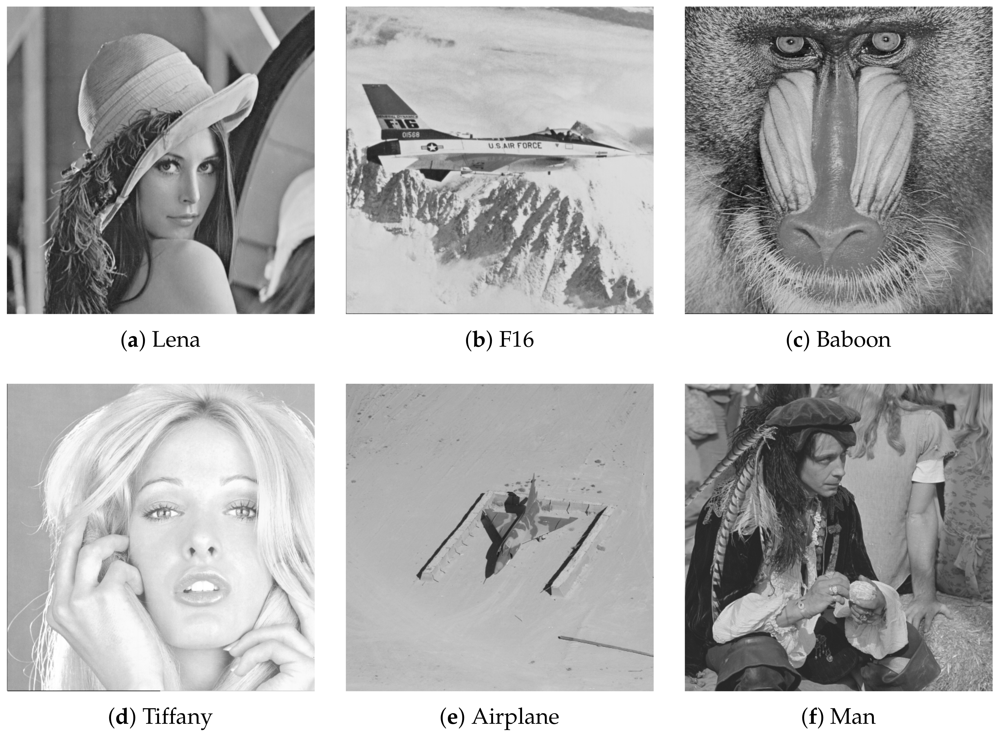
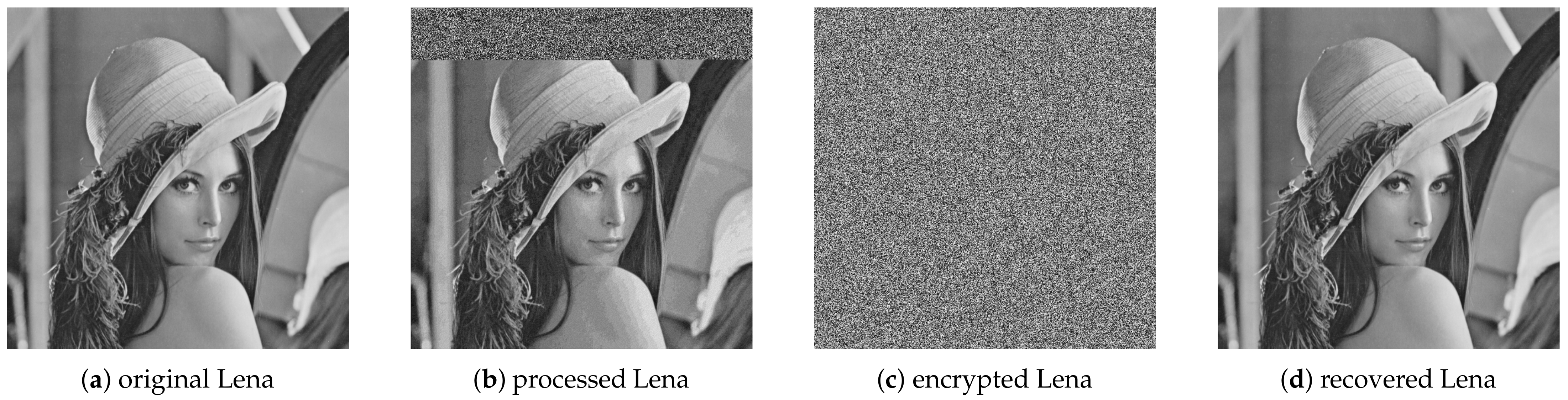
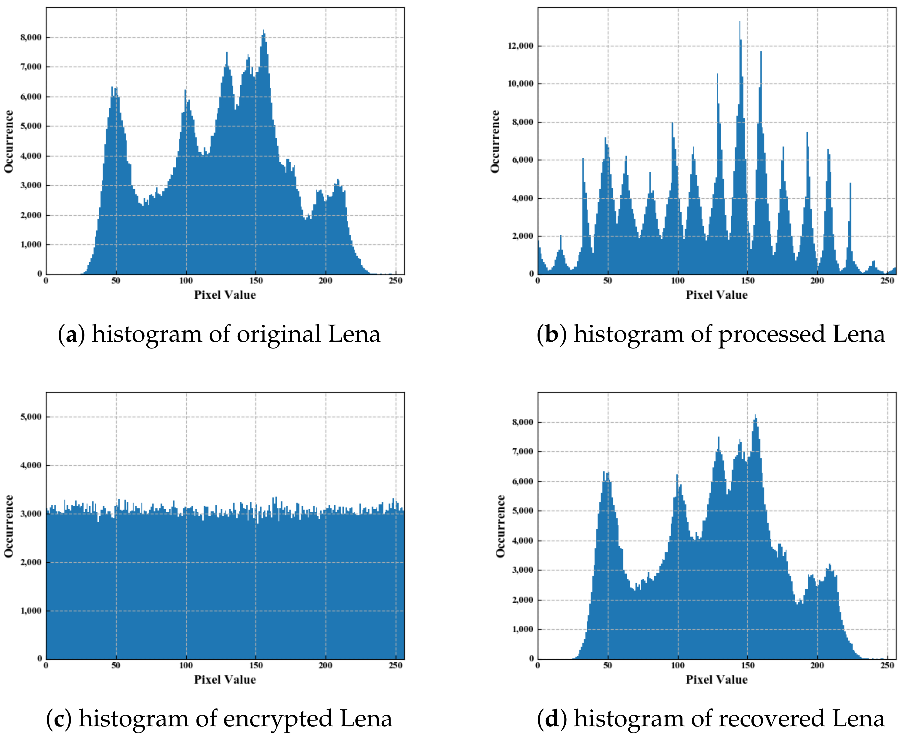
3. Experimental Results and Analysis

In this section, six test images with sizes of 512 × 512 are used to analyze the proposed method based on its different performances. As shown in Figure 6, the test images are Lena, F16, Baboon, Tiffany, Airplane, and Man. The proposed method was implemented in Python 3.7, and the experimental environment was an Intel(R) Core (TM) i-5-8265U CPU @ 1.60 GHz (Intel, Santa Clara, CA, USA) on a Windows 10 PC with 8.0 GB RAM and an NVIDIA GeForce MX350 graphics card (NVIDIA, Santa Clara, CA, USA). Comparisons between the proposed method and the state-of-the-art methods are made in this section. The results are described below.

3.1. Performance and Security Analysis

In the RDHEI method, the privacy of the original image is important to the content owner. To test the security of our method, Lena is used as an example and the parameter $\alpha$ = 4. Figure 7 shows the results of the experiment at different stages. Figure 7a shows the original Lena, and Figure 7b shows the processed Lena. We can observe that the top area of the processed Lena is scrambled; this occurred because the total bitstream $B_t$ is embedded into the consecutive MSBs of the pixels. On the other hand, we label the two’s complement in pixels by LSB, so the remaining area of the processed Lena is similar to the original Lena. In Figure 7c, one can use the encryption key to see the encrypted image. Obviously, no information about the original image can be obtained from Figure 7c, which proves that the proposed method is safe. In addition, Figure 7d shows the recovered Lena after the decryption method. The proposed method is completely reversible, and the peak signal-to-noise rate (PSNR) between Figure 7a,d is $+\infty$ dB. Additionally, in experimental results, the embedded data are extracted without error.

To further verify the safety of the proposed method, a statistical analysis was performed on Lena at different stages in Figure 7. Figure 8 shows the results, where Figure 8a–d are the corresponding histograms of Figure 7a–d. It is apparent that the histogram of the processed Lena (Figure 8b) retains a certain correlation with the original Lena (Figure 8a). After encryption, Figure 8c shows a uniform distribution of the pixels of the encrypted Lena. Thus, it is impossible to obtain the original content about Lena through statistical analysis, which means that the proposed method achieves a high level of security. Indeed, the histogram in Figure 8d shows that the recovered image is lossless.

In the methods of [36,37], the labels of all pixels are shared with the data hider as auxiliary information. However, the prediction error has a one-to-one correspondence with the label. On the other hand, the number of prediction errors is the same as the number of labels. Then, it can be found by statistical analysis that there is a strong correlation between the histogram of the labels and the histogram of the prediction errors. Thus, the auxiliary information in these methods can leak the information of the original image to the data hider. However, in the proposed method, the data hider embeds data through two parameters. In addition, the two’s complement labeled in the image is encrypted, so the data hider cannot obtain the label of each pixel. Thus, the proposed method can achieve higher security.

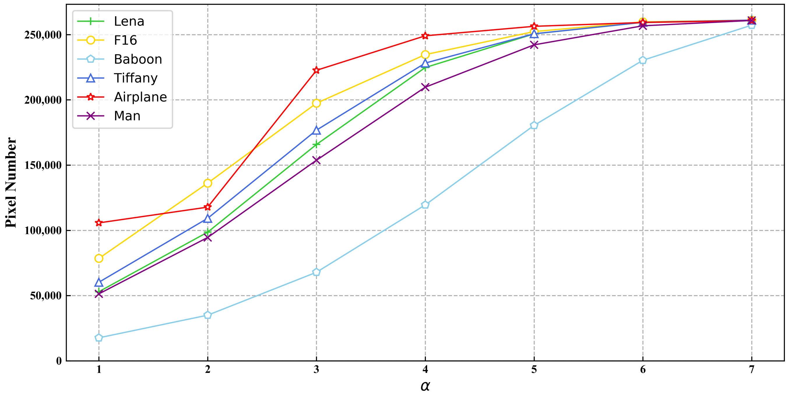
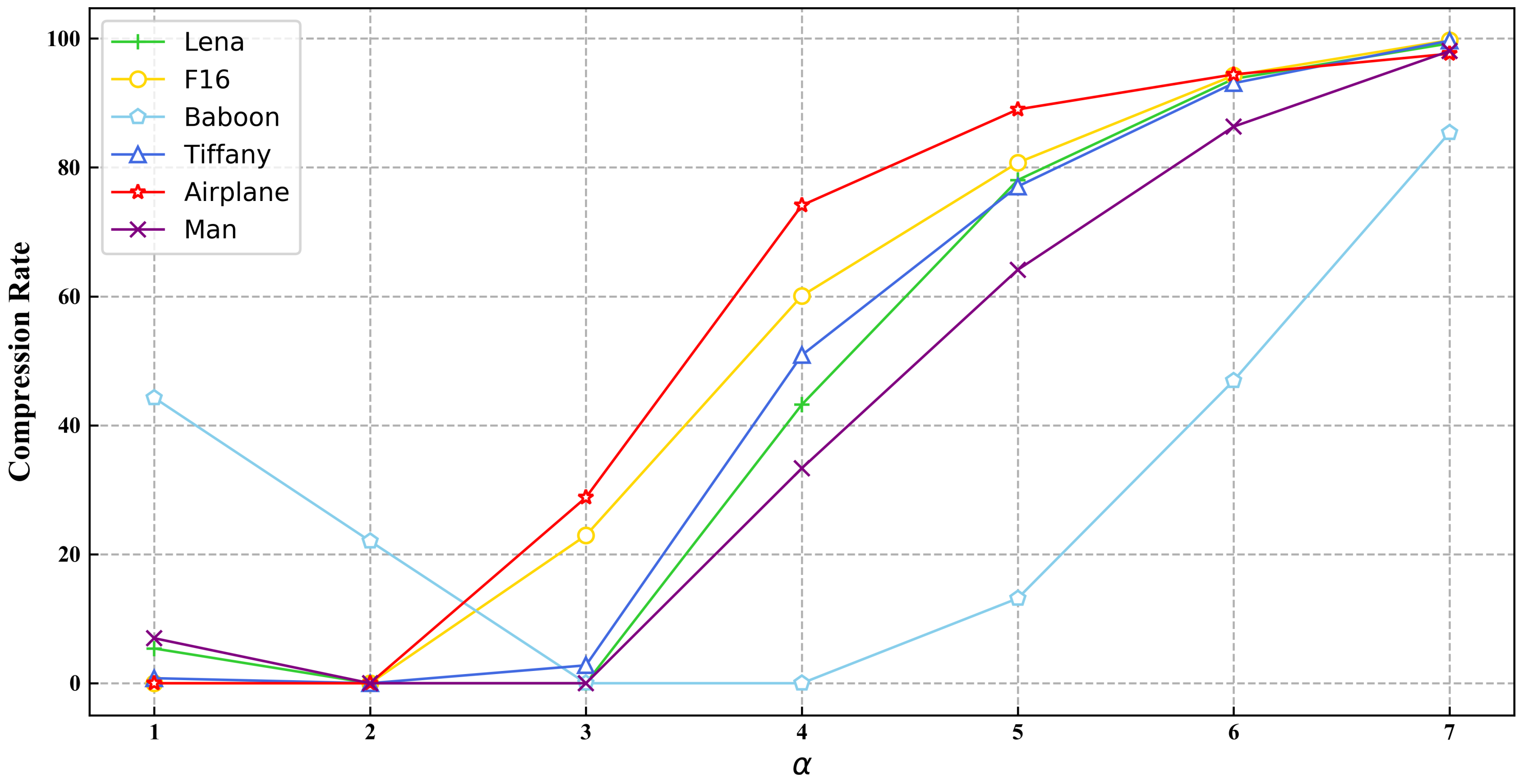
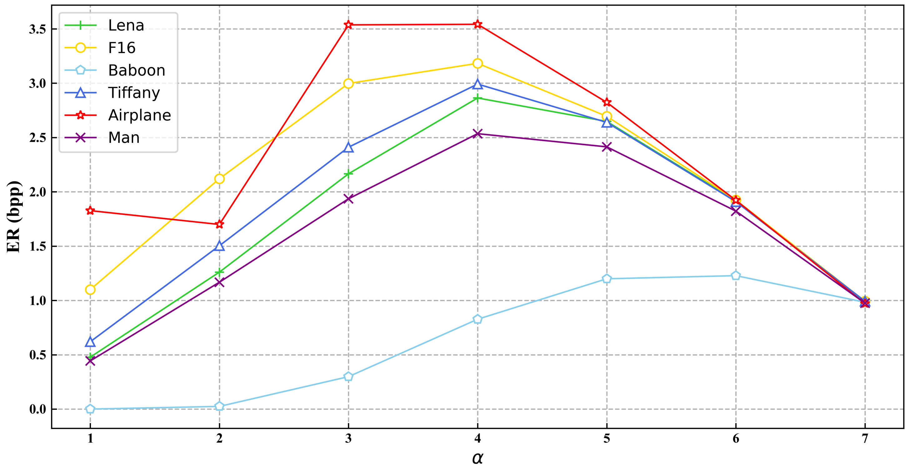
3.2. Parameter and Capacity Analysis

In the proposed method, $\alpha$-bit two’s complement is used to encode the prediction errors. As mentioned before, the range of the coded prediction errors varies with the modification of $\alpha$. To analyze the influence of $\alpha$, there are three different aspects, which are the labeled pixels’ number, the label map’s compression rate, and the ER. Meanwhile, $\alpha$ is chosen from 1 to 7 to experiment on the test images. The experimental results and analysis are as follows.

Table 2. The labeled pixels’ number of each test image under various $\alpha$.

Images	$\mathit{\alpha }$
	1	2	3	4	5	6	7
Lena	52,994	98,612	165,803	224,748	250,541	259,355	261,001
F16	78,498	136,187	197,413	234,660	252,290	259,738	261,079
Baboon	17,670	35,004	67,880	119,490	180,413	230,304	257,215
Tiffany	60,236	109,227	176,759	228,156	250,614	259,381	261,080
Airplane	105,722	117,784	222,628	249,050	256,318	259,248	260,700
Man	51,328	94,551	153,736	209,676	242,126	256,714	260,812

shows the number of labeled pixels in each test image when $\alpha$ takes different values. To better display the data of Table 2, Figure 9 is generated to show how the number of labeled pixels varies with $\alpha$. It can be observed from Figure 9 that the number of labeled pixels increases as $\alpha$ increases. In addition, the number of labeled pixels is close to the total number of pixels in each image when $\alpha$ = 7. For example, the number of labeled pixels in Tiffany is 261,080 when $\alpha$ = 7, while the total number of pixels except the reference pixel is 261,121. In the proposed method, the pixel’s prediction error is easier to fall into the interval represented by $\alpha$-bit complement when $\alpha$ is large. Thus, the larger the value of $\alpha$, the greater the number of labeled pixels.

Moreover, to make the distribution of prediction errors steeper, the MED prediction method is used in this paper.

Table 3. The label map’s compression rate of each test image under different $\alpha$.

Images	$\mathit{\alpha }$
	1	2	3	4	5	6	7
Lena	5.93%	0%	0%	43.22%	78.043%	93.74%	99.24%
F16	0%	0%	22.94%	60.09%	80.74%	94.25%	99.73%
Baboon	44.27%	22.05%	0%	0%	13.16%	46.93%	85.39%
Tiffany	0.783%	0%	2.78%	50.89%	77.05%	93.08%	99.68%
Airplane	0%	0%	28.82%	74.12%	89%	94.44%	97.65%
Man	6.98%	0%	0%	33.35%	64.19%	86.33%	98.05%

shows the compression rate of the label map in each image when $\alpha$ is different. Similarly, to better visualize the change in compression rate, we convert the data in Table 3 into the broken lines in Figure 10. As shown in Figure 10, it can be seen that the trend of the label map’s compression rate is to first decrease and then increase as $\alpha$ increases. The reason is that the proportion of 0 in the label map changes. When the $\alpha$ is small, the proportion of 0 in the label map is small (few labeled pixels). However, the proportion of 1 in the label map is large at this time, which can be compressed. Therefore, the label map has a certain compression rate. For example, the compression rate of Baboon’s label map can reach up to 44.27%. Then, the proportion of 0 in the label map increases as $\alpha$ increases, making the number of 0 and 1 become equal. Thus, the compression rate of the label map is reduced. However, with the proportion of 0 in the label map gradually approaching the maximum as $\alpha$ increases, the label map can be compressed well. For example, the label map’s compression rate of 5 test images is around 99% when $\alpha$ = 7.

In the proposed method, a suitable $\alpha$ can make a large number of labeled pixels to reserve room. Thus, it is very suitable to use the extended run-length coding [34] to compress the label map.

The ER is the most important indicator to measure an RDHEI method. To obtain the maximum ER of test images, all ERs under different $\alpha$ are calculated, which is shown in

Table 4. The ER (bpp) of each test image under different $\alpha$.

Images	$\mathit{\alpha }$
	1	2	3	4	5	6	7
Lena	0.478	1.261	2.166	2.864	2.648	1.916	0.988
F16	1.100	2.121	2.998	3.183	2.695	1.924	0.993
Baboon	$NA$	0.025	0.299	0.827	1.200	1.288	0.836
Tiffany	0.620	1.504	2.411	2.992	2.639	1.910	0.993
Airplane	1.827	1.700	3.537	3.542	2.824	1.923	0.971
Man	0.444	1.168	1.936	2.535	2.414	1.822	0.976

. Further, Figure 11 is generated to visually display the data in Table 4. It is obvious that the ER increases first and then decreases as $\alpha$ increases from 1 to 7. The ER of each test image is not high when $\alpha$ is small, because the labeled pixels’ number and label map’s compression rate are low. As $\alpha$ increases, the labeled pixels’ number and the label map’s compression rate gradually increase ($\alpha$ > 3), so the ER gradually increases. However, the reserved room on each labeled pixel is (8 − $\alpha$) bits. Thus, the room reserved by each labeled pixel decreases as $\alpha$ increases. When $\alpha$ exceeds a certain threshold, the reduced reserved room of the previously labeled pixels is greater than the increased reserved room. Thus, the ER gradually becomes smaller. To maximize the ER, it is necessary to find a suitable $\alpha$ to balance labeled pixels’ number, label map’s compression rate, and each labeled pixel’s reserved room.

In conclusion, $\alpha$ has an important influence on the ER. To achieve the maximum ER, each image needs to choose the appropriate $\alpha$ according to its characteristics. Based on the above experimental results and analysis, the proposed method can achieve the maximum ER when $\alpha$ = 4.

3.3. Comparisons with State-of-the-Art Methods

To verify the superiority of the proposed method, the proposed method is compared with four previous RDHEI methods, i.e., those of [33,34,36,37]. To achieve good performance, multiple bit planes are used for the method of [33]. In the method of [34], the length of the codewords and block size are set to 3 and $4\times 4$, respectively. In the method of [36], parameters $\alpha$ and $\beta$ are selected as 5 and 2, respectively, while the block size is set to $3\times 3$. Similarly, in the improved method of [37], parameters $\alpha$ and $\beta$ are set to 5 and 3. In the proposed method, the most suitable value of parameter $\alpha$ is chosen for each image.

Figure 12 shows the comparison of the maximum ERs on the six test images of the proposed method with these four methods. It can be observed that the ER of each image obtained by the proposed method is higher than that of other methods. Furthermore, the ERs on F16 and Airplane of other methods do not exceed 3 bpp, but the ERs of the proposed method reach 3.1 bpp and 3.5 bpp, respectively. Obviously, the proposed method can significantly improve the ER on smooth images. Meanwhile, in these comparative methods, the ER of Baboon is very low. However, the proposed method can achieve an ER of 1.2 bpp on Baboon, indicating that our method also has good performance on rough images.

To reduce the influence of the test images on the outcome of the comparison, the proposed method is applied to three datasets when $\alpha$ is set to 4, i.e., UCID [40] (Avilable online: http://vision.doc.ntu.ac.uk/, accessed on 2 July 2020), BOSSbase [41] (Avilable online: http://dde.binghamton.edu/download/, accessed on 18 May 2021), and BOWS-2 [42] (Avilable online: http://bows2.ec-lille.fr/, accessed on 18 May 2021). The detailed ERs of the three datasets are shown in

Table 5. The experimental results of three datasets when $\alpha$ = 4.

Datasets	Minimum ER	Maximum ER	Average ER
UCID	0.117	3.924	2.578
BOSSbase	0.165	3.984	3.041
BOWS-2	0.091	3.984	2.941

. From the results, it can be seen that the maximum ERs of the different datasets are close to 4 bpp, while the minimum ERs are greater than 0 bpp. Thus, these experimental results confirm the universality of the proposed method.

Moreover, we compare the average ERs on the different datasets between the proposed method and the four works, as shown in Figure 13. From the figure, it can be observed that the proposed method has higher average ERs on the datasets than other methods. In particular, in the dataset BOSSbase, the average ER of our method exceeds 3 bpp. From the above comparison, it is obvious that the proposed method can achieve a higher ER than existing state-of-the-art methods.

4. Conclusions

In this paper, we propose a new RDHEI method based on MED and two’s complement. First, the MED prediction method is used to predict the pixels in the image. Then, the prediction errors between the original pixels and the predicted values can be obtained. Based on the distribution of the prediction errors, an appropriate interval is encoded by $\alpha$-bit two’s complement. According to experimental results and analysis, the appropriate value of $\alpha$ is 4 or a similar value. To reserve room in the image, two’s complement of the prediction error is labeled in the pixel by LSB. Then, a label map is generated to distinguish labeled and unlabeled pixels. To ensure that the original image can be restored losslessly, we use an MSB rearrangement method to embed the label map in the image as auxiliary information. After encrypting the processed image, we can embed secret data in the encrypted image. During the decoding phase, the secret data can be extracted correctly through the data hiding key. Meanwhile, using the image encryption key, the original image can be recovered from the marked encrypted image losslessly, as shown in the experimental results. Thus, the proposed method satisfies the reversibility of the original image. Moreover, the comparisons of experimental results prove that the proposed method can achieve a higher ER than previous methods.

In the future, we plan to increase the ER in two ways. On the one hand, an efficient coding scheme can be used to label more prediction errors. On the other hand, the auxiliary information can be reduced by improving the compression method.

References

1. Bender, W.; Gruhl, D.; Morimot, N.; Lu, A. Techniques for data hiding. IBM Syst. J. 1996, 35, 313–336. [Google Scholar] [CrossRef]
2. Chan, C.K.; Cheng, L.M. Hiding data in images by simple LSB substitution. Pattern Recognit. 2004, 37, 469–474. [Google Scholar] [CrossRef]
3. Celik, M.; Sharma, G.; Tekalp, A.; Saber, E. Lossless generalized-LSB data embedding. IEEE Trans. Image Process. 2005, 14, 253–266. [Google Scholar] [CrossRef] [PubMed]
4. Tian, J. Reversible data embedding using a difference expansion. IEEE Trans. Circuits Syst. Video Technol. 2003, 13, 890–896. [Google Scholar] [CrossRef] [Green Version]
5. Tai, W.L.; Yeh, C.M.; Chang, C.C. Reversible data hiding based on histogram modification of pixel differences. IEEE Trans. Circuits Syst. Video Technol. 2009, 19, 906–910. [Google Scholar]
6. Lin, C.C.; Liu, X.L.; Tai, W.L.; Yuan, S.M. A novel reversible data hiding scheme based on AMBTC compression technique. Multimedia Tools Appl. 2015, 74, 3823–3842. [Google Scholar] [CrossRef]
7. Malik, A.; Singh, S.; Kumar, R. Recovery based high capacity reversible data hiding scheme using even-odd embedding. Multimedia Tools Appl. 2018, 77, 15803–15827. [Google Scholar] [CrossRef]
8. Kumar, R.; Chand, S.; Singh, S. An optimal high capacity reversible data hiding scheme using move to front coding for LZW codes. Multimedia Tools Appl. 2019, 78, 22977–23001. [Google Scholar] [CrossRef]
9. Dragoi, I.C.; Coltuc, D. Local-prediction-based difference expansion reversible watermarking. IEEE Trans. Image Process. 2014, 23, 1779–1790. [Google Scholar] [CrossRef] [PubMed]
10. Arham, A.; Nugroho, H.A.; Adji, T.B. Multiple layer data hiding scheme based on difference expansion of quad. Signal Process. 2017, 137, 52–62. [Google Scholar] [CrossRef]
11. Wang, W.; Ye, J.; Wang, T.; Wang, W. Reversible data hiding scheme based on significant-bit-difference expansion. IET Image Process. 2017, 11, 1002–1014. [Google Scholar] [CrossRef]
12. Pan, Z.; Hu, S.; Ma, X.; Wang, L. Reversible data hiding based on local histogram shifting with multilayer embedding. J. Vis. Commun. Image Represent. 2015, 31, 64–74. [Google Scholar] [CrossRef]
13. Wang, J.; Ni, J.; Zhang, X.; Shi, Y.Q. Rate and distortion optimization for reversible data hiding using multiple histogram shifting. IEEE Trans. Cybern. 2016, 47, 315–326. [Google Scholar] [CrossRef] [PubMed]
14. Jia, Y.; Yin, Z.; Zhang, X.; Luo, Y. Reversible data hiding based on reducing invalid shifting of pixels in histogram shifting. Signal Process. 2019, 163, 238–246. [Google Scholar] [CrossRef] [Green Version]
15. Kumar, R.; Chand, S.; Singh, S. A reversible data hiding scheme using pixel location. Int. Arab. J. Inf. Technol. 2018, 15, 763–768. [Google Scholar]
16. Kumar, R.; Chand, S.; Singh, S. An Improved Histogram-Shifting-Imitated reversible data hiding based on HVS characteristics. Multimed. Tools Appl. 2018, 77, 13445–13457. [Google Scholar] [CrossRef]
17. Kumar, R.; Chand, S.; Singh, S. A reversible high capacity data hiding scheme using combinatorial strategy. Int. J. Multimedia Intell. Secur. 2018, 3, 146–161. [Google Scholar] [CrossRef]
18. Zhang, W.; Wang, H.; Hou, D.; Yu, N. Reversible Data Hiding in Encrypted Images by Reversible Image Transformation. IEEE Trans. Multimed. 2016, 18, 1469–1479. [Google Scholar] [CrossRef]
19. Yang, C.T.; Shih, W.C.; Chen, G.H.; Yu, S.C. Implementation of a cloud computing environment for hiding huge amounts of data. In Proceedings of the International Symposium on Parallel and Distributed Processing with Applications, Taipei, Taiwan, 6–9 September 2010; pp. 1–7. [Google Scholar]
20. Abbasy, M.R.; Shanmugam, B. Enabling data hiding for resource sharing in cloud computing environments based on DNA sequences. In Proceedings of the 2011 IEEE World Congress on Services, Washington, DC, USA, 4–9 July 2011; pp. 385–390. [Google Scholar]
21. Hwang, K.; Li, D. Trusted cloud computing with secure resources and data coloring. IEEE Int. Comput. 2010, 14, 14–22. [Google Scholar] [CrossRef]
22. Xiong, L.; Shi, Y. On the privacy-preserving outsourcing scheme of reversible data hiding over encrypted image data in cloud computing. Comput. Mater. Contin. 2018, 55, 523–539. [Google Scholar]
23. Qin, C.; Zhang, X. Effective reversible data hiding in encrypted image with privacy protection for image content. J. Vis. Commun. Image Represent. 2015, 31, 154–164. [Google Scholar] [CrossRef]
24. Puech, W.; Chaumont, M.; Strauss, O. A reversible data hiding method for encrypted images. In Proceedings of the Security, Forensics, Steganography, and Watermarking of Multimedia Contents X, San Jose, CA, USA, 18 March 2008; pp. 534–542. [Google Scholar]
25. Zhang, X. Reversible data hiding in encrypted image. IEEE Signal Process. Lett. 2011, 18, 255–258. [Google Scholar] [CrossRef]
26. Hong, W.; Chen, T.S.; Wu, H.Y. An improved reversible data hiding in encrypted images using side match. IEEE Signal Process. Lett. 2012, 19, 199–202. [Google Scholar] [CrossRef]
27. Ma, K.; Zhang, W.; Zhao, X.; Yu, N.; Li, F. Reversible data hiding in encrypted images by reserving room before encryption. IEEE Trans. Inf. Forensics Secur. 2013, 8, 553–562. [Google Scholar] [CrossRef]
28. Mathew, T.; Wilscy, M. Reversible data hiding in encrypted images by active block exchange and room reservation. In Proceedings of the 2014 International Conference on Contemporary Computing and Informatics, Mysore, India, 27–29 November 2014; pp. 839–844. [Google Scholar]
29. Zhang, W.; Ma, K.; Yu, N. Reversibility improved data hiding in encrypted images. Signal Process. 2014, 953, 118–127. [Google Scholar] [CrossRef]
30. Puteaux, P.; Trinel, D.; Puech, W. High-capacity data hiding in encrypted images using MSB prediction. In Proceedings of the 2016 Sixth International Conference on Image Processing Theory, Tools and Applications, Oulu, Finland, 12–15 December 2016; pp. 1–6. [Google Scholar]
31. Puteaux, P.; Puech, W. An efficient MSB prediction-based method for high-capacity reversible data hiding in encrypted images. IEEE Trans. Inf. Forensics Secur. 2018, 13, 1670–1681. [Google Scholar] [CrossRef] [Green Version]
32. Puyang, Y.; Yin, Z.; Qian, Z. Reversible data hiding in encrypted images with two-MSB prediction. In Proceedings of the 2018 IEEE International Workshop on Information Forensics and Security, Hong Kong, China, 11–13 December 2018; pp. 8–15. [Google Scholar]
33. Puteaux, P.; Puech, W. EPE-based huge-capacity reversible data hiding in encrypted images. In Proceedings of the 2018 IEEE International Workshop on Information Forensics and Security, Hong Kong, China, 11–13 December 2018; pp. 1–7. [Google Scholar]
34. Chen, K.; Chang, C.C. High-capacity reversible data hiding in encrypted images based on extended run-length coding and block-based MSB plane rearrangement. J. Vis. Commun. Image Represent. 2019, 58, 334–344. [Google Scholar] [CrossRef]
35. Yin, Z.; Xiang, Y.; Zhang, X. Reversible data hiding in encrypted images based on multi-MSB prediction and Huffman coding. IEEE Trans. Multimed. 2019, 22, 874–884. [Google Scholar] [CrossRef]
36. Yi, S.; Zhou, Y. Separable and reversible data hiding in encrypted images using parametric binary tree labeling. IEEE Trans. Multimed. 2019, 21, 51–64. [Google Scholar] [CrossRef]
37. Wu, Y.; Xiang, Y.; Guo, Y.; Tang, J.; Yin, Z. An improved reversible data hiding in encrypted images using parametric binary tree labeling. IEEE Trans. Multimed. 2020, 22, 1929–1938. [Google Scholar] [CrossRef] [Green Version]
38. Yin, Z.; Niu, X.; Zhang, X.; Tang, J.; Luo, B. Reversible data hiding in encrypted AMBTC images. Multimedia Tools Appl. 2018, 77, 18067–18083. [Google Scholar] [CrossRef]
39. Shiu, P.F.; Tai, W.L.; Jan, J.K.; Chang, C.C.; Lin, C.C. An interpolative AMBTC-based high-payload RDH scheme for encrypted images. Signal Process. Image Commun. 2019, 74, 64–77. [Google Scholar] [CrossRef]
40. Schaefer, G.; Stich, M. UCID: An uncompressed color image database. In Proceedings of the Storage and Retrieval Methods and Applications for Multimedia 2004, San Jose, CA, USA, 18 December 2003; pp. 472–480. [Google Scholar]
41. Bas, P.; Filler, T.; Pevny, T. Break our steganographic: The ins and outs of organizing BOSS. In Proceedings of the International Workshop on Information Hiding, Berlin, Germany, 18–20 May 2011; pp. 59–70. [Google Scholar]
42. Image Databased of BOWS-2. Available online: http://bows2.ec-lille.fr/ (accessed on 1 April 2021).
Figure 1. The framework of the proposed method.
Symmetry 13 00921 g001
Figure 2. The context of the MED predictor.
Symmetry 13 00921 g002
Figure 3. Illustrative example of pixel labeling.
Symmetry 13 00921 g003
Figure 4. Illustrative example of two’s complement labeling process.
Symmetry 13 00921 g004
Figure 5. Illustrative example of the processed image.
Symmetry 13 00921 g005
Figure 6. The test images.
Symmetry 13 00921 g006
Figure 7. The different images of Lena generated by the proposed method.
Symmetry 13 00921 g007
Figure 8. The histograms of pixel values of Lena in each step.
Symmetry 13 00921 g008
Figure 9. The labeled pixels’ number of test images under various α .
Symmetry 13 00921 g009
Figure 10. The compression rates of label maps under various α .
Symmetry 13 00921 g010
Figure 11. The embedding rates of test images under various α .
Symmetry 13 00921 g011
Figure 12. Comparison of maximum embedding rates of test images.
Symmetry 13 00921 g012
Figure 13. Comparison of the average embedding rates of three datasets.
Symmetry 13 00921 g013