Mathematical Algorithm for Identification of Eukaryotic Promoter Sequences

Abstract

Identification of promoter sequences in the eukaryotic genome, by computer methods, is an important task of bioinformatics. However, this problem has not been solved since the best algorithms have a false positive probability of 10⁻³–10⁻⁴ per nucleotide. As a result of full genome analysis, there may be more false positives than annotated gene promoters. The probability of a false positive should be reduced to 10⁻⁶–10⁻⁸ to reduce the number of false positives and increase the reliability of the prediction. The method for multi alignment of the promoter sequences was developed. Then, mathematical methods were developed for calculation of the statistically important classes of the promoter sequences. Five promoter classes, from the rice genome, were created. We developed promoter classes to search for potential promoter sequences in the rice genome with a false positive number less than 10⁻⁸ per nucleotide. Five classes of promoter sequences contain 1740, 222, 199, 167 and 130 promoters, respectively. A total of 145,277 potential promoter sequences (PPSs) were identified. Of these, 18,563 are promoters of known genes, 87,233 PPSs intersect with transposable elements, and 37,390 PPSs were found in previously unannotated sequences. The number of false positives for a randomly mixed rice genome is less than 10⁻⁸ per nucleotide. The method developed for detecting PPSs was compared with some previously used approaches. The developed mathematical method can be used to search for genes, transposable elements, and transcript start sites in eukaryotic genomes.

1. Introduction

The promoter sequences, in both prokaryotes and eukaryotes, are located up to the point of transcription initiation [1]. The site on the DNA from which the first RNA nucleotide is transcribed is called the +1 site. The so-called core promoter, with a length of 60–120 bases, stands out, and RNA polymerase binds to this DNA region [2,3]. A longer stretch of 600 bases from −499–+100 includes the core promoter, as well as the binding sites of various transcription factors [4]. “Further, we will focus only on eukaryotic promoter sequences. The promoter includes some motifs, which are short conservative sequences. The so-called TATA sequence is known, which occupies positions from −31–−26 nucleotides [5]. Additionally, the B recognition element is known, which is between −37 and 32 nucleotides in the promoter sequence. Short sequences have been found that provide binding of various protein factors to the promoter sequence [6]. Many of these sequences fall on the promoter region from +1–+40. The promoter sequence is not symmetrical” [7], thereby making the DNA polymerase begin transcription in the right direction.

Promoter sequences are very different from each other [8,9,10]. This is as a result of the need to control the transcription of various genes. When transcription is initiated, the transcription initiation complex is assembled [11]. The complex includes RNA polymerase, a promoter sequence, and “dozens of other transcription factors. The set of these factors can vary from one gene to another, which in turn leads to a strong variety of promoter sequences. Today, hundreds of thousands of promoter sequences from various eukaryotic genomes are known” [7]. Databases have been created for promoter sequences [4]. In this work, 4220 promoters from the rice genome were used, after obtaining them from the site http://linux1.softberry.com/data/plantprom/Links/PLPR_predicted_OS.seq (accessed on 19 May 2021). We chose the rice genome for study, as it is well annotated [12] and the agricultural value of rice is very high. However, despite such a large number of promoter sequences, it has not been possible to find a statistically significant multiple alignment between them [13]. This resulted in the difficulty associated with identifying (annotating) promoters using a nucleotide sequence. A typical scheme for annotating different nucleotide or amino acid sequences is to construct a statistically significant multiple alignment for sequences that perform the same genetic functions. “Then this alignment is used for profile analysis or for constructing a hidden Markov model. Such a scheme leads to a low number of false positives when annotating genomes. However, algorithms for predicting promoter sequences currently use other mathematical methods due to the lack of statistically significant multiple alignment” [7]. These algorithms include TSSW [9], PePPER [14], G4PromFinder [15], deep learning approach [16], method based on evolutionarily generated patterns [17] and many others. The best algorithms have false positive probability of 10⁻³–10⁻⁴ per nucleotide. The rice genome contains ~4.3 × 10⁸ DNA base, and more than 4 × 10⁴ false positives will be generated using well-known methods. The probability of a false positive could be reduced to 10⁻⁶–10⁻⁸ to reduce the number of false positives and increase the reliability of the prediction. If promoter sequences can be correctly predicted, then genes and transcription start sites (TSS) could be more accurately identified.

In this work, multiple alignment for promoter sequences from the rice genome was performed and “a mathematical method for calculating multiple alignment for highly different sequences (MAHDS) was developed” [7]. Multiple alignment for nucleotide sequences may be calculated on the site http://victoria.biengi.ac.ru/mahds/auth (accessed on 19 May 2021) [18]. A method for creating promoter classes, based on multiple alignment, was also developed. In total, 5 classes of promoter sequences were created for which the volume of classes was more than 100 promoters. “The obtained classes of promoter sequences were used to search for other promoter sequences in the rice genome” [19]. A profile matrix a_m(16,600) was calculated for each class. Using dynamic programming, a search for potential promoter sequences was carried out for each matrix. In the sequence of chromosome S, the S₃(k) window with the size of 650 bases was selected, and we searched for the best intersection of the matrix a_m(16,600) and the S₃(k) sequence (see below, Section 2.4.). We took into account the correlation of neighboring base pairs, and, for this, we used 16 rows in the a_m(16 600) matrix. Window S₃(k) moved in increments of 10 bases throughout the rice genome. In this study, 145,277 potential promoters were found. Of these, 18,563 are promoters of known genes, which is about 46% of the annotated genes. The number of false positives for the randomly mixed rice genome was about 10⁻⁸ per nucleotide. “At the same time, the correlation of the found potential promoter sequences (PPSs) with various dispersed repeats and transposons was studied. It was possible to show that ~87 thousand PPSs correlate with various dispersed repeats and transposons [12]. Other PPSs may be promoters of unknown genes, micro RNA genes [20], promoters associated with various mobile elements of the genome, as well as evolutionary traces of the resettlement of genes and their promoters” [19].

2. Materials and Methods

2.1. Promoter Sequences from the Rice Genome

A total of 4220 promoters, from the rice genome, were taken from http://linux1.softberry.com/berry.phtml?topic=plantprom&group=data&subgroup=plantprom (accessed on 19 May 2021). These promoters range from −200–+51 DNA bases near transcription start site. For this study, we obtained sequences from −499–+101 around the same 4220 transcription start sites. To achieve this, each of the 4220 promoter sequences in the rice genome were found and a region from −499–+100 was selected. We used the rice genome sequences from http://plants.ensembl.org/Oryza_sativa/Info/Index (accessed on 19 May 2021). Consequently, 4220 promoter sequences were obtained, by which promoter classes were created. The set of these sequences was denoted as Q, and each promoter sequence as S(i), i = 1, 2, …, N. The volume of the set Q was equal to N = 4220. Each promoter “had a length of 600 nucleotides. The promoter included sequences from −499–+100” [7] relative to the transcription start site (+1 position).

2.2. Multiple Alignment of Promoter Sequences from the Rice Genome by the MAHDS Method

To perform multiple alignment, we did the concatenation of V_Q = 100 randomly selected sequences, from the set Q, into one sequence S₁ of length K = 600 V_Q. A small value of V_Q allows us to accelerate the global alignment and all calculations. First, let us take a look at the general scheme for creating multiple alignments using the MAHDS method, shown in Figure 1 [18]. Thereafter, some of the points shown in Figure 1 will be considered in more detail below in separate paragraphs. The MAHDS method does not use direct calculation of multiple alignment by any comparison of sequences from the set Q. The main idea is to use multiple alignment images in the form of position-weight matrices to calculate multiple alignment (Figure 1, point 2) [18]. Initially, we generated random position-weight matrices (PWM). These matrices are calculated using random sequences obtained by the random mixing of promoter sequences from the Q set. The calculation of random PWM’s were done according to the Equations (1) and (2). The position-weight matrix contains 599 columns and 16 lines. The number of rows is equal to the number of pairs of nucleotides. Then these matrices are transformed in a certain way, and a set of matrices A is created that contains V_A matrices. The essence of the transformation is to ensure that the sum of the squares of all elements of each matrix and K_d (Equations (3) and (4)) are constants for the whole A set. The creation of positional weight matrices from the A set is considered in Section 2.3.

Then the positional weight matrices from the A set are optimized by the genetic algorithm (Figure 1, points 3–5). The goal of this optimization is to create a PWM that has the best global alignment with the S₁ sequence [21,22]. By the best alignment, we mean an alignment that will have the greatest value of the function F_o = F(K,K). Here, F(K,K) is the value of the similarity function at the point (K,K) of the dynamic programming matrix. In more detail, the global alignment of the matrix a(i) from the A set and the sequence S₁ is discussed below in Section 2.4. Each matrix a(i) has 599 columns and 16 lines.

The genetic algorithm contains three steps. In the first stage (Figure 1, point 3), each matrix a(i) from the A set is aligned with the sequence S₁. As a result, for each matrix, F_o is calculated and the vector F_o(i), i = 1, 2, …., V_A, is created. In the second stage (Figure 1, point 4), the vector F_o(i) is arranged in descending order, so that F_o(1) is its maximum element. We take F_m = F_o(1) and denote the matrix that corresponds to F_m as a_m. F_o(i) is considered as an objective function, and the matrices a(i) as organisms for the genetic algorithm. Our task is to maximize F_m. This is achieved by introducing mutations into matrices from the A set. This is the third stage of the genetic algorithm, which is shown in Figure 1, point 5. For this, 1% of the matrices a(i) from the A set is randomly selected. Then for these matrices, we randomly, and equally likely, select the number of mutations from 1–10. Then, for each mutation, a cell of the a(i) matrix which has size 16 × 600 is randomly selected. Thereafter, we randomly and equally likely select a new value for the matrix cell in the range from −10.0–+10.0. The genetic algorithm is shown in [23]. The application of the genetic algorithm for multiple alignment of nucleotide sequences is described in detail in [18].

Simultaneously, with the introduction of mutations, one descendant is created instead of the matrix a (V_A), which has the smallest value of the similarity function F_o(V_A). In addition, 0.5% of the matrices exchanged their randomly selected parts, which was a kind of crossing-over for these “organisms”. The descendant and crossing over were created as in [23]. If F_m > F₁ then we do F₁ = F_m and we go back to point 3, Figure 1. If F_m ≤ F_1, and this has already been going on for at least 10 times (Figure 1, point 7), then we go to point 8 and create a multiple alignment of the promoter sequences from the Q set. The multiple alignment is calculated by global alignment of the sequence S₁ with respect to the a_m matrix. The construction of multiple alignment is considered below in Section 2.5.

2.3. Creation of Random Matrices from the A Set.

Sequences were randomly mixed from the Q set and the Q_r set was created. Each sequence from the Q_r set also had a length equal to 600 bases. Thereafter, the sequences were placed under each other and got multiple alignments without insertions and deletions with the number of rows N = 4220 and with the number of columns equal to N_s = 600. Then the probability of occurrence of the bases was calculated as p(i) = n(i)/K₂. Here n(i) is the number of bases of type i in all sequences from the created multiple alignment, i$\in${a,t,c,g}. K₂ = N_sN = 600 × 4220—is the total length of all sequences in the Q_r set. Then, the probabilities of finding a base pair f(i,j) = p(i)p(j), j$\in${a,t,c,g} were calculated. Here, t(i,j,k) was also calculated; this is the number of pairs (i,j) at positions k–1 and k, k varies from 2–N_s. Then we calculated:

$$x(i,j,k)=\frac{t(i,j,k)-Nf(i,j)}{\sqrt{Nf(i,j)(1-f(i,j))}}$$

(1)

where Nf(i,j) is the expected number of the neighboring base pair (i,j), and x(i,j,k) is the cell of the a(1) matrix from the A set. Thus, the first matrix a(1) was filled from the A set. The first column of the matrix a(1) was also filled as:

$$x(i,j,1)=\frac{t(i,1)-Np(i)}{\sqrt{Np(i)(1-p(i))}}$$

(2)

where t(i,1) is the number of bases i in the first column of the created multiple alignment. This formula is valid for j$\in${a,t,c,g}, j$\in${a,t,c,g}. The volume V_A of the A set was 1000 sequences. Thereafter, each matrix from the A set was transformed. The created matrices were transformed so that R² and K_d were the same and equal to 55,000 and −1.5, respectively. The constants R and K_d can be calculated using the following Equations (3) and (4):

$$R^2={\displaystyle \sum _{i=1}^{16}{\displaystyle \sum _{j=2}^{N_s}a}}{(i,j)}^2$$

(3)

$$K_d={\displaystyle \sum _{t=1}^{16}{\displaystyle \sum _{k=2}^{N_s}a}}(t,k)p_1(t)p_2(k)$$

(4)

where $p_2\left(k\right)=1/599$, p₁(t) = p(l)p(m), (l,m $\in$ {a,t,c,g}) and p(l) and p(m) are the probabilities of the l or m type nucleotides in Q set; $p_2\left(k\right)=1/599$. The matrix transformation procedure is described in details in [23]. The transformation was done so that the calculated F₀(i) would have a similar distribution when random sequences are aligned. Thus, the best a_m matrix can be found based on the similarity function (F_m) and the p-value was not calculated. This greatly facilitated the computation.

2.4. Global Alignment of PWM and Sequence S₁

First, let us define the sequence S₂. This sequence contains 1, 2, …, 599 which is repeated V_Q = 100 times. The length of the sequence S₂ (as well as the sequence S₁) is K = 600V_Q. The symbols of the sequence S₁ were denoted as s₁(i), and the symbols of the sequence S₂ as s₂(i), i can vary from 1–K. Then the sequence S₁ was aligned with the matrices a from the A set. The matrix cell was denoted as a(i,j), with i varying from 1–16, j from 1–599. The sequence S₁ was encoded according to the following rule: A = 1, T = 2, C = 3, G = 4, where A, T, C and G are DNA bases. F is calculated as:

$$\begin{array}{l}F(i,j)=\max \left\{\begin{array}{l}F(i-1,j-1)+a(n,s_2(j))\\ F_x(i-1,j-1)+a(n,s_2(j))\\ F_y(i-1,j-1)+a(n,s2(j))\end{array}\right\}\\ \end{array}$$

(5)

$$\begin{array}{l}{F}_x(i,j)=\max \left\{\begin{array}{l}F(i-1,j)-d\\ F_x(i-1,j)-e\end{array}\right\}\\ \end{array}$$

(6)

$$\begin{array}{l}{F}_y(i,j)=\max \left\{\begin{array}{l}F(i,j-1)-d\\ F_y(i,j-1)-e\end{array}\right\}\\ \end{array}$$

(7)

Initial conditions: F(0,0) = 0.0, F(i,0) = F(0,i) = –di. Here n = s₁(k) + 4(s₁(i)–1), i runs from 2–K and j runs from 2–K. For i = 1, n = s₁(1). The element s₁(i) is of the sequence S₁ and s₂(i) is an element of the sequence S₂. a(i,j) is an element of the a matrix from the A set. The parameter n takes into account the correlation of bases in the matrix a. The previous position (k) must be calculated, which has already been included in the alignment. Therefore, the index k was calculated from the already created transitions in the F matrix, depending on the previous base of S₁ that was included in the alignment. Depending on the index k, we took a(n,s₂(i)). If the previous base of the sequence S₁ is s(i–t), then k = i–t and n = s₁(i–t) + (s₁(i)–1)*4 are taken. t = 1 corresponds to movement along the main diagonal of the F matrix. In this case, there is no deletion in the S₁ sequence in the alignment. t > 1 corresponds to a deletion of the t–1 bases in the sequence S₁.

Deletions may also occur in the S₂ sequence. Deletions in the S₂ sequence correspond to deletions of columns in the matrix a. If the previous symbol in the sequence S₂, which we took in alignment, has the number j–1, then there are no deletions in the sequence S₂. If this number is j–t (t > 1) then this corresponds to a deletion of t–1 bases in the sequence S₂. For these transitions, the correlations of adjacent bases were not considered. This is quite acceptable in cases with a relatively small number of deletions. In this case we took n = s₁(i) and s₂(j) = 1 in Equation (5).

We took, d = 35.0 and e = 8.0. Selection of the insertion/deletion penalty was performed as in our earlier work [23], using the study of model sequences. The reverse transition matrix was filled along with the F matrix. Therefore, the alignment of the sequences S₁ and S₂ was built using the reverse transition matrix and the F(K,K) was determined. The alignment of the S₁ and S₂ sequences was calculated for all matrices from the A set. As a result, the vector F_o(i), i = 1,…,V_A containing F(K,K) for each of the matrices was obtained.

2.5. Calculations of Multiple Alignment from Two-Dimensional Alignment of the Sequences S1 and S2

We obtained the matrix a_m, which has the highest value of F_m when aligning with the sequence S₁ as a result of the algorithm for constructing multiple alignment. The algorithm is shown in Figure 1. This alignment is depicted as a juxtaposition of the positions of the columns (sequence S₂) with nucleotides of the sequence S₁. In the S₁ sequence, V_Q = 100 promoter sequences from the rice genome are arranged one after another. In fact, the task was to create multiple alignment from the two-dimensional alignment of sequences S₁ and S₂ for promoter sequences from the Q set. The construction of multiple alignment involves a two-step cyclic process. Step 1. k = 1. First, we find all s₂(i) = k, i = 1, 2, …, K, K = 600V_Q. There are V_Q = 100 such values. All those bases or deletions of bases that are in the sequence S₁ opposite s₂(i) = k are written in the current column of the matrix MA starting from the first. Deletions of bases are denoted by *. Step 2. Thereafter, we consider the bases in the sequence S₁ opposite which are located * in the sequence S₂. Asterisks should be located between s₂(i) = k and s₂(i) = k + 1 in the sequence S₂, i = 1, 2, …, K. Then additional columns should be introduced in the MA matrix. In these columns, we write, in turn, all the bases from the sequence S₁ located opposite the asterisks. The number of columns is equal to the length of the longest fragment in the sequence S₁, which is located opposite asterisks (**...*) in the sequence S₂. These asterisks on the left are bounded by s₂(i) = k, and on the right, s₂(i) = k + 1. Then we do k = k + 1 and repeat all the calculations. The process is stopped if k > 600. In the case k = 600, the asterisks should be located between s₂(i) = 600 and s₂(i) = 1 in the sequence S₂, i = 1, 2, …, K in step 2.

Consider a small example. Suppose K = 15 and the alignment of sequences S₁ and S₂ is:

$$\begin{array}{c}\mathrm{1**23451*2345123*45}\\ \mathrm{atcgtcaagg*caagtgca}\end{array}$$

(8)

Then multiple alignment is:

$$\begin{array}{c}\mathrm{1**23*45}\\ \mathrm{atcgt*ca}\\ \mathrm{ag*g**ca}\\ \mathrm{a**gtgca}\end{array}$$

(9)

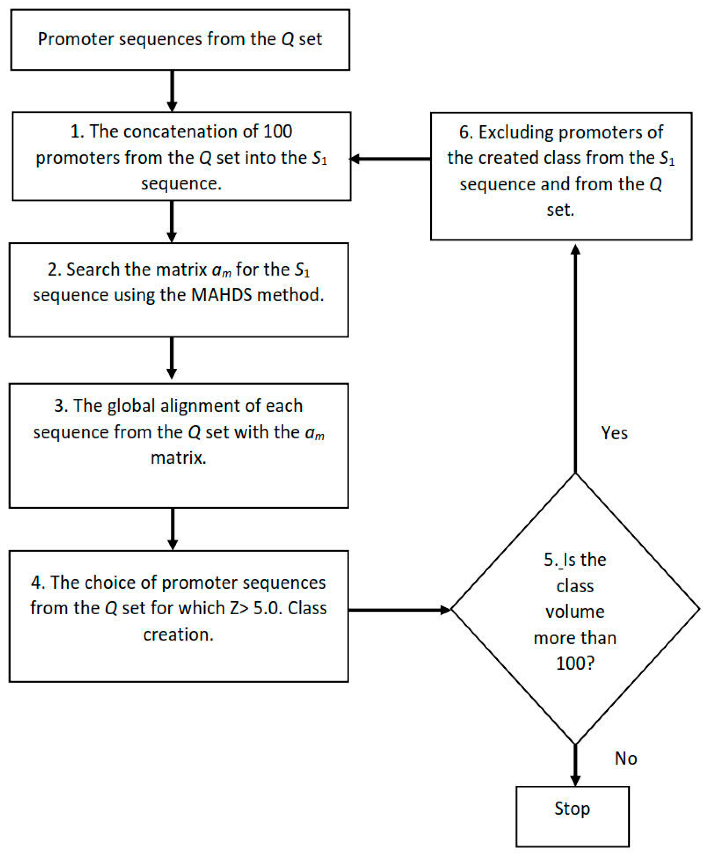
2.6. Creating Classes of Promoter Sequences

The algorithm for creating classes is shown in Figure 2. The V_Q of randomly selected promoter sequences from the Q set was combined into the sequence S₁ as we wrote about it above. The choice of V_Q = 100 is based on the fact that for V_Q > 100, the time for calculating global alignment increases significantly. Then the matrix a_m was calculated as described in Section 2.5. (Figure 2, point 1,2). “However, only part of the promoter sequences from the Q set can have a statistically significant alignment with the a_m matrix” [7]. There are two reasons for this; first, V_Q is less than the number of promoters in the Q set (N = 4220) and most of the promoters were not included in the S₁ sequence. Secondly, a certain number of promoters in the sequence S₁ may not have statistically significant alignment with the matrix a_m.

Therefore, each promoter sequence S(i) (i = 1, 2, …, N) from the Q set was aligned with respect to the matrix a_m (Figure 2, point 3). This way, only those promoter sequences that have a statistically significant alignment with the matrix a_m were selected. The alignment algorithm was the same as in Section 2.4. In this case, K = 600, V_Q = 1. Instead of the sequence S₁, we only analyzed one after another sequence S(i) from the Q set. For each sequence from the Q set, we calculated F(K,K) (Section 2.2).

The statistical significance of the resulting alignments was estimated. For this, random Q_r sequences were used (Section 2.3). Each sequence from the set Q_r was aligned and the value of F(K,K) for each sequence was calculated. Thus, 4220 F(K,K) for randomly mixed sequences were obtained. For this set of the F(K,K), the mean $\overline{F(K,K)}$ and variance $D(F(K,K))$ were calculated.

In this study, $Z=\{F(K,K)-\overline{F(K,K)}\}/\sqrt{D(F(K,K))}$ was calculated for each promoter from the Q set. If the promoter sequence S(i) from the Q set has Z > 5.0, then it is written in the class of promoter sequences that can be detected using the matrix a_m (Figure 2, point 4).

Thus, part of the promoter sequences from the Q set was written into the created class. Then we checked that the created class has more than 100 sequences. The minimum size of classes equal to 100 was defined, based on random sequence analysis (Figure 2, point 5). “When this procedure was performed on random sequences, the volume of classes ranged from 0–27 sequences with an average value of 16 sequences” [18]. This means that the probability of creating a class of 100 sequences, due to random factors, is negligible.

Then the promoters included in the created class from the Q set (Figure 2, point 6) were excluded. We moved to point 1 of Figure 2 and the procedure for creating a class of promoter was repeated again. As a result, the algorithm shown in Figure 2 was used to calculate the matrix a_m and multiple alignment of 100 sequences for which the a_m matrix was created. The alignment of each promoter sequence included in the created class was calculated with respect to the a_m matrix.

We found the maximum of x(i,j,k), k varies from 2–600 (Equation (1)) for the calculated multiple alignment of 100 sequences (on the basis of which the matrix a_m was created). For each position k, the base pair of 16 having the largest value x(i,j,k) was chosen. This value was denoted as X(k) and the dependences of X(k) on k for the first two classes of promoter sequences were calculated.

To do this, we calculated the probabilities of nucleotide bases p(i) (i = 1,2,3,4) for multiple alignment of each class. Then, for each position j in multiple alignment, we calculated the number of nucleotides y(i,j). We only took the positions of multiple alignment, where the number of nucleotides was >10. The number of such positions for all multiple align classes is 600. For each position j, we calculated m(j) = ${\displaystyle \sum _{i=1}^{4}y(i,j)}$. Then we calculated x(i,j) = (y(i,j)–m(j)p(i))/($\sqrt{m(j)p(i)(1-p(i))}$. To build a consensus in each position j, we took that nucleotide (i), which had the greatest value x(i,j). If x(i,j) was <1.0, we took N into the position j. Thus, 5 consensus sequences were built for each class.

2.7. Search for Potential Promoter Sequences in the Rice Genome

On each chromosome, the S₃(k) sequence with a length of 650 bases (K₁ = 650) was selected. Here, k varied from 1–Chl–649 in increments of 10 bases, where Chl is the chromosome length. The sequence S₃(k) was aligned with respect to the columns of the matrix a_m (sequence S₂) for the created classes of promoter sequences. The alignment algorithm was the same as in Section 2.4, but with minor changes. Here, i can vary from 1–K₁, and j can vary from 1–K, K = 600. The initial conditions for filling the matrix F are different: F(i,0) = F(0,j) = 0.0, i = 0, 1, …, K₁, j = 0, 1, …, K. After filling the F matrix, we searched for a maximum in the rows F(i,K) and F(K₁,j),), i = 0, 1, …, K₁, j = 0, 1, …, K. Suppose we find the maximum of F at the point (i_m,j_m); from this point using the reverse transition matrix, we build the alignment of the sequences S₃(i) and S₂ before crossing with F(i,0) and F(0,j), i = 0, 1, …, K₁, j = 0, 1, …, K. This means that the best intersection of the sequence S₃(k) and S₂ is found. Then Z was calculated as in Section 2.6 for each k from 1–Chl–649 in increments of 10 bases. As a result, an array of Z_l (k) was obtained. Here, the index l shows the class number of the promoter sequences. In our case, l varied from 1–5, since 5 classes of promoter sequences were created.

Z_l(k) was also calculated for each of the inverted chromosomes and these arrays were denoted as $Z_l^{inv}(k)$. All local maxima, no closer than 600 bases from each other (intersection no more than 0%), were identified. We took the local maximum of the intersecting ones, having the largest value of Z_l(k) and more than 5.0. This search for PPSs was performed for all 12 rice chromosomes. As a result, for each chromosome we have the coordinates of the PPSs, alignment of the PPSs with the class matrix a_m, Z for the PPSs, the class number, and the DNA strand (direct or complementary).

3. Results

3.1. Classes of Promoter Sequences from the Rice Genome

Five statistically significant classes of promoter sequences, with class volume 1740, 222, 199, 167, and 130 promoters, were created. This is consistent with the estimated class number of promoters in eukaryotic genomes [24]. All classes contained about 60% of the selected rice promoters (a total of 4220 sequences were used). The remaining 40% are in smaller classes. It can be observed that the first class is the largest, containing about 1740 of the 4220 promoters.

The conservation of bases in the first two classes of promoter sequences was studied. In Figure 3 and Figure 4 (black circles), we plotted the dependence X(k), k = 1, 2, …, 599 for the first two classes of promoter sequences. At the same time, the dependence X(k) for randomly mixed sequences was calculated. The multiple alignment created for the class of promoter sequences was recorded and the nucleotides were randomly mixed. Here, the position of the insertions or deletions were unchanged. The obtained graphs are shown in Figure 3 and Figure 4 (white circles).

Figure 3 shows that the promoter sequences of the first class from the rice genome have some base pairs for which X(k) is greater than X(k) for randomly mixed sequences. The probability of X(k) to be greater than 5.0 is less than 10⁻⁵. A conserved promoter sequence can be noticed in the region of k = 475, which corresponds to the TATA region of the promoter [20]. The most significant base pairs were found in positions from +1–+80. This may be due to both transcription initiation [1] and translation initiation [25]. It is likely that certain transcription or translation factors need only certain DNA bases or only certain combinations of them (or motifs). Therefore, a strong increase in X(k) was observed for k > +1 in Figure 3.

However, this phenomenon was not observed for the second class of promoter sequences (Figure 4). The values of X(k) in the second class for k > +1 are not much greater than X(k) for all other k. This may indicate that there are either different mechanisms of transcription initiation, of different genes in the rice genome, or different factors of initiation of both transcription and translation. It is also important to note that, for promoter sequences, X(k) from −499–+1 is greater than for random sequences. This may indicate that many DNA motifs in this region are important for the binding of transcription factors [26].

Also, the difference between X(k) obtained for promoter sequences and X(k) calculated for random sequences, was investigated. To do this, N(X) was calculated, which shows the number of X(k) from X–+∞. In total, there are 599 X(k) for each class of promoter sequences, therefore N(X) varies from 0–599. For the first and second classes of promoter sequences, the dependences of N(X) on X are shown in Figure 5 and Figure 6. These figures show that N(X), in the interval x from 0.0–3.0, is more than 2–5 times greater for promoter sequences than for random sequences. Comparing Figure 3 and Figure 4, as well as 5 and 6, it can be said that the difference in the alignment of promoter sequences from random sequences occurs both due to several tens of X(k) > 3.0, and due to several hundred X(k) between 0.0 and 3.0.

A total of 4220 promoters from the PlantProm DB 18 database (Q set) were used to create promoter sequence classes. These promoter sequences were detected by both experimental and theoretical methods. It is difficult to completely exclude the possibility that a certain number of sequences that are not promoters are in the Q set. As can be seen from the results, only about half of the 4220 sequences from Q set were included in the created classes. All sequences that did not enter into multiple alignment for each of the 5 classes (Figure 1 and Figure 2) were eliminated. When creating the classes, it was assumed that “pollution” of up to 20–40% does not have a significant effect on the created classes. This was tested by replacing the promoter sequences from the Q set with random sequences. It was found that the created classes were unaffected by replacing 25% of the sequences in the Q set with random sequences. With 50% random sequences in the Q set, only the first class of promoter sequences can be constructed. Therefore, the real similarity of promoters in the rice genome is believed to be reflected by the classification created.

3.2. PPS in the Rice Genome

The calculated a_m matrices for 12 chromosomes from the rice genome, were searched for PPSs as described in Section 2.7. Chromosome sequences of the rice genome were taken from http://plants.ensembl.org/Oryza_sativa/Info/Index (accessed on 19 May 2021). The results of this study are shown in

Table 1. The number of potential promoter sequences (PPS’s) found in rice chromosomes. The following four PPS intersections were limited to regions of −499–+100. ++ is the number of PPS intersections for annotated genes. +− is the number of PPS intersections for annotated genes on a complementary strand. −+ is the number of PPS intersections on a complementary strand for annotated genes. −− is the number of PPS intersections on a complementary strand for annotated genes on a complementary strand. R is the number of PPS’s in the sequence of randomly mixed chromosomes. M is the number of PPS’s in the inverted sequence of chromosomes.

Chromosome	Number of Genes	Number PPS	++	+−	−+	−−	R	M
1	5350	21,960	1271	246	109	1485	0	62
2	4296	13,497	1116	106	121	1058	0	17
3	4648	13,121	1337	61	170	817	1	54
4	3429	14,775	963	46	170	640	0	39
5	3070	11,034	479	150	18	981	1	40
6	3204	11,381	713	87	51	849	0	31
7	2917	10,016	824	55	62	697	0	18
8	2636	10,223	849	23	97	481	0	33
9	2144	7575	579	15	87	275	0	6
10	2184	7943	204	124	11	664	0	3
11	2663	11,648	630	39	91	512	0	33
12	2215	12,104	597	69	83	542	0	11
All	38,756	145,277	9562	1021	1070	9001	2	347

. The coordinates of the annotated genes were taken from the site: http://plants.ensembl.org/info/data/ftp/index.html (accessed on 19 May 2021). The search for PPS was carried out by the sequences of two DNA strands. The sequence of the second strand was sequence which was complemented and reversed. A control search PPS in random sequences was also conducted, as well as in inverted sequences (without recoding to the complementary sequence).

The results for PPSs search in the rice chromosomes are shown in Table 1. From this Table, it can be seen that the number of PPSs is 3–5 times higher than the number of known genes in each chromosome. If these results are summarized for the entire rice genome, then 145,277 PPSs will be found, whereas the rice genome contains 38,756 annotated genes. The low level of false positives (FP) that we were searching for in the mixed chromosomes of rice or in inverted sequences, should also be noted. The number of false positives (FP) for randomly mixed rice genome is 2 (Table 1). If the fact that the Oryza sativa genome has approximately 430 megabases in size [27] is considered, then the probability of false positives for the search of PPS is 2/430 × 10⁶ < 10⁻⁸ per nucleotide. If false positives are evaluated by inverted sequences (Table 1), then the probability of false positives is 347/430 × 10⁶ < 10⁻⁶ per nucleotide. The achieved probability of false positives is approximately 3–4 orders of magnitude lower than that of all previously developed programs, and this allows us to analyze the complete rice genomes and identify PPSs without significant random noise.

20,654 of sites were found from −499–+100 for annotated genes, as shown in Table 1. This is the sum of matches ++, +−, −+, −− in Table 1. Classes were created for approximately 60% of the 4220 promoter sequences from the Q set. Therefore, it seems very logical that about half of the promoter sequences around known genes (this is sum of matches ++ and −−) have been identified in the right direction. The number of such promoters is 18,563. This is an argument in favor of the fact that the classification was carried out correctly. This means that classes for the set Q are common to all promoter sequences from the rice genome. It can also be noticed that about 2000 promoter sequences around annotated genes were identified in the opposite direction (Table 1). This may indicate the existence of bidirectional promoters in the rice genome [28,29]. It can be partially explained by fluctuations in the calculation of Z using the Monte Carlo method, as well as by overlapping promoter sequences on two DNA strands.

The number of PPS intersecting with the promoter sequences for each class is shown in

Table 2. The number of PPS intersections with promoter sequences from the rice genome. The first column shows the class of PPS’s. The following four PPS intersections were limited to regions of −499–+100. ++ is the number of PPS intersections for annotated genes. +− is the number of PPS intersections for annotated genes on a complementary strand. −+ is the number of PPS intersections on a complementary strand for annotated genes. −− is the number of PPS intersections on a complementary strand for annotated genes on a complementary strand.

Class Number	++	+−	−+	−−
1	6133	456	561	4955
2	792	195	145	958
3	1169	144	163	1218
4	755	101	112	700
5	713	125	89	1170

. It can be seen that the most known promoter sequences can be found by the first class. This number is about 6–8 times more compared to the remaining 4 created classes. It can be said that the number of intersections with known promoters for each class is proportional to the number of promoters included in each class.

The density of PPSs in various rice chromosomes was also studied. The highest density is present on the first chromosome of rice, as shown in the Figure 7. The first chromosome has the average distance between the PPSs equal to 2 × 10³ bases and the lowest density was observed in the 9th chromosome of rice. The 9th chromosome has one PPS for ~3 × 10³ DNA bases.

3.3. The Intersection of PPS with Known Promoters and Transposons

The main question that arises from Table 1 is why there are so many PPSs, almost 4 times more than annotated genes. We thought that these PPSs could be associated with LTR, mobile elements, SINE, and LINE repeats. Therefore, the intersection of PPSs with the transposable elements (TEs), identified in [12], was studied. TE and PPSs are considered intersecting if they intersect at 80% or more of the length of any of them, as shown in

Table 3. The intersections of the PPS with transposons in the rice genome.

N	Name of Dispersed Repeat OT Transposon	Number of Intersections	The Expected Number of Intersections	X1
1	DNAnona/Helitron	7466	7044	5.03
2	DNAnona/unknown	1501	870	21.39
3	MITE/Tourist	10,507	8955	16.40
4	MITE/Stow	9891	8189	18.81
5	DNAauto/MULE	2140	2792	−12.34
6	DNAnona/MULE	12,288	9531	28.24
7	LINE/unknown	2153	4045	−29.75
8	LTR/Gypsy	18,043	22,837	−31.72
9	DNAnona/hAT	3824	3616	3.46
10	DNAnona/MULEtir	3328	1793	36.25
11	DNAnona/Tourist	917	463	21.10
12	LTR/Copia	2675	4736	−29.95
13	DNAauto/CACTA	1265	1967	−15.83
14	SINE/unknown	1252	1666	−10.14
15	DNAnona/CACTA	3736	2395	27.40
16	DNAauto/hAT	438	479	−1.87
17	DNAnona/PILE	426	403	1.15
18	DNAauto/PILE	259	251	0.50
19	LTR/TRIM	190	705	−19.40
20	DNAauto/Helitron	226	487	−11.83
21	Evirus/ERTBV-C	39	45	−0.89
22	LTR/unknown	119	232	−7.42
23	DNAnona/CACTG	1141	675	17.94
24	DNAauto/CACTG	2614	2503	2.22
25	LTR/Solo	36	15	5.42
26	DNAauto/MLE	154	182	−2.08
27	Evirus/ERTBV-B	21	59	−4.95
28	Evirus/ERTBV-A	22	45	−3.43
29	Evirus/ERTBV	23	20	0.67
30	DNAauto/POLE	161	168	−0.54
31	DNAnona/POLE	253	168	6.56
32	DNAnona/MLE	32	44	−1.81
33	Centro/tandem	93	298	−11.88

. TEs on each rice chromosome were mixed, and the number of intersections with the PPS for different TEs was counted. This was done 100 times. As a result, the expected number of intersections and variances, for the random arrangement of TEs in rice chromosomes, were calculated. Thereafter, $X_1=\{C-\overline{C}\}/\sqrt{D(C)}$ was calculated. “Here, C is the number of PPS intersections with TEs in the rice genome, $\overline{C}$ is the expected number of PPS intersections with TEs, D(C) is the variance for the expected number of PPS intersections with TEs” [30]. The location of some TEs is strongly correlated with the PPS locations, as shown in Table 3. This is most noticeable for MULEtir, MULE and some other transposons.

If the total number of intersections is calculated, then a maximum of 87,233 PPSs are associated with TEs. If 20,654 PPSs associated with promoters of annotated genes are added to this amount, then 107,887 PPSs are associated with the already annotated sequences. However, there are 37,390 PPSs that occurred in previously unannotated sequences. In part, these may be promoters for micro RNAs, which are also transcribed by RNA polymerase-II [31,32], as well as promoters of unknown genes.

The intersection of the classes of PPS with TE is shown in

Table 4. Table shows the number of intersections of transposons with PPS’s, which were obtained using various position-weight matrices. Matrix classes are shown as columns M1, M2, …, M5.

N	Name of Dispersed Repeat ot Transposon	M1	M2	M3	M4	M5
1	DNAnona/Helitron	3015	1540	795	1089	1027
2	DNAnona/unknown	670	268	176	136	251
3	MITE/Tourist	4507	1850	1329	1216	1605
4	MITE/Stow	5376	1208	894	944	1469
5	DNAauto/MULE	948	370	311	240	271
6	DNAnona/MULE	6201	1982	1362	1377	1366
7	LINE/unknown	813	328	383	293	336
8	LTR/Gypsy	9877	2610	2333	1903	1320
9	DNAnona/hAT	1883	615	411	438	477
10	DNAnona/MULEtir	1528	629	486	323	362
11	DNAnona/Tourist	441	154	151	80	91
12	LTR/Copia	839	447	484	522	383
13	DNAauto/CACTA	564	170	204	187	140
14	SINE/unknown	653	170	132	140	157
15	DNAnona/CACTA	1823	542	492	482	397
16	DNAauto/hAT	241	37	61	57	42
17	DNAnona/PILE	211	53	54	38	70
18	DNAauto/PILE	91	49	48	40	31
19	LTR/TRIM	85	24	30	22	29
20	DNAauto/Helitron	100	34	24	23	45
21	Evirus/ERTBV-C	1	12	12	11	3
22	LTR/unknown	50	17	15	18	19
23	DNAnona/CACTG	670	169	107	121	74
24	DNAauto/CACTG	757	611	353	654	239
25	LTR/Solo	15	6	3	8	4
26	DNAauto/MLE	65	22	35	10	22
27	Evirus/ERTBV-B	5	5	1	6	4
28	Evirus/ERTBV-A	10	3	2	4	3
29	Evirus/ERTBV	2	8	2	1	10
30	DNAauto/POLE	59	22	37	19	24
31	DNAnona/POLE	108	38	45	29	33
32	DNAnona/MLE	16	5	6	1	4
33	Centro/tandem	6	31	1	43	12
	Total:	41,630	14,029	10,779	10,475	10,320

. For the matrix of the first class, the number of such intersections is 41,630, and for the 4 remaining classes it is 14,029, 10,779, 10,475, and 10,320, respectively. The specificity of all 5 PPS classes was evaluated for different TEs. Let columns 1 and 2 be eliminated from Table 4 and the remaining matrix considered as M(i,j), i = 1, 2, …, 5, j = 1, 2, …, 33; then, $X_2=\{M-\overline{M}\}/\sqrt{D(M)}$ is counted. Here M is the number of PPS intersections with TEs in the rice genome for each matrix, $\overline{M}$ is the expected number of PPS intersections with TEs for each matrix, D(M) is the variance for the expected number of PPS intersections with TEs for each matrix.

Here, $\overline{M}$ is calculated as X(i)Y(j)/Sum, where X(i), i = 1, 2, …, 5, is the sum of the M(i,j) for j = 1, 2, …, 33. Y(j), j = 1, 2, …, 33, is the sum of the M(i,j) for i = 1, 2, …, 5. Only those rows in Table 4, where there is at least one element for which X₂ > 6.0 and M(i,j) > 100 were considered. The results of these calculations are shown in

Table 5. Table shows the deviation of the number of intersections of PPSs with transposons using the various position-weight matrices from the expected number of intersections. Each cell contains an X₂ which is an argument of the normal distribution. If X₂ is greater than 6.0, then there is a correlation between transposons and PPS. The promoter classes are shown as columns M1, M2, …, M5. Only those rows are shown where X₂ > 6.0. The numbering of the first column in the table corresponds to the numbering of the first column in the Table 4.

N	Name of Dispersed Repeat ot Transposon	M1	M2	M3	M4	M5
1	DNAnona/Helitron	−9.3738	9.8600	−4.2215	6.4616	4.8613
3	MITE/Tourist	−7.3783	3.9365	0.8583	−1.2957	10.3410
4	MITE/Stow	9.8136	−9.6839	−9.4540	−7.1205	8.7958
7	LINE/unknown	−6.7306	−0.9827	7.1819	2.1467	5.1011
8	LTR/Gypsy	14.3752	−5.5078	2.2207	−5.7351	−17.8504
12	LTR/Copia	−12.3378	0.8120	8.4570	11.2236	3.7471
24	DNAauto/CACTG	−13.9871	9.3190	1.6723	19.2314	−4.0017

.

It can be seen that the PPS detected using the M1 matrix are most specific for LTR/Gypsy and MITE/Stow. PPS detected using the M2 matrix are most specific for DNAnona/Helitron and DNAauto/CACTG. As can be seen from Table 5, specificity was also observed for other matrices. It can be assumed that the classes of promoter sequences may be associated with various groups of biological processes.

4. Discussion

The results obtained in this paper were compared with some other algorithms and programs. Initially, the Neural Network Promoter Prediction (NNPP) was used [33]. For this, a set of 100 randomly selected promoter sequences was obtained from the rice genome (R1 set) as well as 100 randomly mixed sequences of the same length (R2 set). In the R1 set, NNPP found 78 promoter sequences, and for the R2 set there were 68 of such sequences. It is clear that the number of false positives for NNPP is very high. Then, TSSW [34] and TSSP [9] algorithms were also tested. TSSP works the same as TSSW, but uses the RegSite database of plant regulatory elements [35]. Moreover, the TSSP algorithm aims to search for promoter sequences in plant genomes. In this case, the R1 set and R2 set each contained 6 × 10⁴ sequences. As a result, 20 sequences from the R1 set and 35 from the R2 set were found by the TSSW program. TSSP found 85 sequences from the R1 set and 24 from the R2 set. That is, the number of false positives here is approximately 0.5 × 10⁻³ per nucleotide. Similar results were obtained for BPROM [9]. Then, in order to study the R1 and R2 sets, PROMOTER2 was applied [36]. Here, volumes of sets equal to 500 sequences were used. The program calculates the Score parameter. If Score >1.0, then it is highly likely that the analyzed sequence is a promoter. In the case of the R1 set, 30 promoter sequences having Score >1.0 were found. In the case of the R2 set, 25 promoter sequences were found. These results show that PROMOTER2 has the large number of false positives and extremely low efficiency of searching for promoters.

It is interesting to discuss the limitations of the approach used to construct multiple alignment in this paper. In this work, approximately 50% of the known promoter sequences were found in the rice genome. This could be due to the fact that promoter sequences may have different lengths or contain oversized (more than 50 nucleotides) insertions or deletions of nucleotides. Then building multiple alignment with the MAHDS program is difficult. This is due to the fact that promoter sequences are combined into one sequence S₁ for constructing multiple alignment. In this case, a large insertion, or deletion, at the beginning of the sequence S₁ will prevent finding the optimal multiple alignment for the sequences that are behind it. This disadvantage can be taken into account when modernizing the MAHDS method. Since the promoter can have different sizes, this will lead to the fact that part of the promoter sequences will be outside the created classes. It was assumed that this is why 5 classes were created that cover approximately 50% of the Q set volume.

It is also interesting to consider why the first class of promoter sequences is several times larger than the remaining classes. First of all, this may be due to the presence of large-sized inserts or deletions in the nucleotide sequences of other classes relative to the first class. This may prevent the association of promoters into one large class at a statistically significant level by the method developed in this work. The presence of such inserts or deletions may be associated with a different set of transcription factors around the genes [37]. If we can improve our approach and reduce the influence of oversize inserts, then we can probably combine all the promoter sequences into one class.

We have created multiple alignments and classes for promoter sequences from the human genome [38] and the A. thaliana genome [18]. For the human genome, it was possible to create 25 classes of promoter sequences, the same number of classes was created for the A. thaliana genome. These classes already cover 75% of the known promoter sequences (~60% in this work, Section 3.1). At present, only the total number of PPS in these genomes has been obtained. For the A. Thalian genome, this amount is comparable to the results obtained for the rice genome (taking into account the size of the genome). In total, about 62 thousand PPS were found. More than 1.0 million PPS have been found in the human genome. These data show that the developed method for creating classes of promoter sequences, and searching for PPS, can be applied to study various genomes.

Consensus sequences for created classes are in the Supplement. It can be seen that the classes of promoter sequences are very different from each other. This is consistent with the fact that promoter sequences from the genome A. thaliana have many mutations, and the average number of replacements on the nucleotide is from 3.6–3.8 per nucleotide [18]. A similar picture is observed for the rice genome. In this case, it is impossible to build pair alignments of promoter sequences.

In general, the results of this work showed that the developed mathematical method can be effective in searching for the promoter sequences in the rice genome. Promoters of previously unknown genes [39,40,41,42], TEs and transcript start sites can be found using the developed method. Of course, the mathematical research was performed, but it opened up certain prospects for experimental work. This particularly concerns 37,390 PPSs which were revealed about unannounced sequences. We only got 347 false positives (FPs) when looking for PPPs in inverted and complementary sequences. Let’s roughly estimate the probability of finding at least 1000 false positives. We will consider FP as a random variable that has a normal distribution. Then the argument of the normal distribution is x ≈ (1000–347)/(347)^0.5 = 35,5. The probability of such an event is certainly much less than 10⁻¹⁰⁰. Therefore, from a mathematical point of view, these 37,390 PPS are not false positives. These PPS can be non-functioning promoter sequences, evolutionary traces of the resettlement of various genes or transposons. On the other hand, these may be promoter sequences of unknown genes, and they may indicate the existence of genes that have not been discovered [42]. Conducting purely experimental work in the future is considered useful in answering this question.

5. Conclusions

In this study, the method for multi alignment of the promoter sequences was developed. Then, mathematical methods were developed for calculation of the statistically important classes of the promoter sequences. Five promoter classes were created from the rice genome. A total of 145,277 potential promoter sequences (PPSs) were found in the rice genome. Of these, 87,233 PPSs are associated with TEs and 20,654 PPSs are associated with promoters of annotated genes. There are 37,390 PPSs that occurred in previously unannounced sequences. The number of false positives for a randomly mixed rice genome is ~10⁻⁸ per nucleotide. It was assumed that these PPSs are associated with unknown genes, with transposable elements, or micro-RNA. In general, the results of this work showed that the developed mathematical method can be effective for searching the promoter sequences in rice genomes. Promoters of previously unknown genes, TEs and transcript start sites can be found using the developed method.

References

1. Nogales, E.; Louder, R.K.; He, Y. Structural Insights into the Eukaryotic Transcription Initiation Machinery. Annu. Rev. Biophys. 2017, 46, 59–83. [Google Scholar] [CrossRef]
2. Juven-Gershon, T.; Hsu, J.-Y.; Theisen, J.W.; Kadonaga, J.T. The RNA polymerase II core promoter—The gateway to transcription. Curr. Opin. Cell Biol. 2008, 20, 253–259. [Google Scholar] [CrossRef] [Green Version]
3. Smale, S.T.; Kadonaga, J.T. The RNA Polymerase II Core Promoter. Annu. Rev. Biochem. 2003, 72, 449–479. [Google Scholar] [CrossRef] [PubMed] [Green Version]
4. Dreos, R.; Ambrosini, G.; Groux, R.; Cavin Périer, R.; Bucher, P. The eukaryotic promoter database in its 30th year: Focus on non-vertebrate organisms. Nucleic Acids Res. 2017, 45, D51–D55. [Google Scholar] [CrossRef] [Green Version]
5. Lodish, H.; Berk, A.; Matsudaira, P.; Kaiser, C.A.; Krieger, M.; Scott, M.P.; Zipursky, L.; Darnell, J. Molecular Cell Biology; Macmillan: New York, NY, USA, 2008; Volume 4, ISBN 0716776014. [Google Scholar]
6. Roeder, R. The role of general initiation factors in transcription by RNA polymerase II. Trends Biochem. Sci. 1996, 21, 327–335. [Google Scholar] [CrossRef]
7. Korotkova, M.A.; Kamionskya, A.M.; Korotkov, E.V. A mathematical method for the classification of promoter sequences from the A.thaliana genome. In Proceedings of the Journal of Physics: Conference Series; IOP Publishing Ltd.: Bristol, UK, 2020; Volume 1686, p. 012031. [Google Scholar]
8. Abeel, T.; Van De Peer, Y.; Saeys, Y. Toward a gold standard for promoter prediction evaluation. Bioinformatics 2009, 25, i313–i320. [Google Scholar] [CrossRef] [PubMed] [Green Version]
9. Solovyev, V.V.; Shahmuradov, I.A.; Salamov, A.A. Identification of promoter regions and regulatory sites. Methods Mol. Biol. 2010, 674, 57–83. [Google Scholar] [CrossRef]
10. Abe, H.; Gemmell, N.J. Abundance, arrangement, and function of sequence motifs in the chicken promoters. BMC Genom. 2014, 15, 1–12. [Google Scholar] [CrossRef] [Green Version]
11. Lee, T.I.; Young, R.A. Transcription of Eukaryotic Protein-Coding Genes. Annu. Rev. Genet. 2000, 34, 77–137. [Google Scholar] [CrossRef] [PubMed]
12. Ou, S.; Su, W.; Liao, Y.; Chougule, K.; Agda, J.R.A.; Hellinga, A.J.; Lugo, C.S.B.; Elliott, T.A.; Ware, D.; Peterson, T.; et al. Benchmarking transposable element annotation methods for creation of a streamlined, comprehensive pipeline. Genome Biol. 2019, 20, 275. [Google Scholar] [CrossRef] [PubMed] [Green Version]
13. Zeng, J.; Zhu, S.; Yan, H. Towards accurate human promoter recognition: A review of currently used sequence features and classification methods. Brief. Bioinform. 2009, 10, 498–508. [Google Scholar] [CrossRef] [PubMed] [Green Version]
14. De Jong, A.; Pietersma, H.; Cordes, M.; Kuipers, O.P.; Kok, J. PePPER: A webserver for prediction of prokaryote promoter elements and regulons. BMC Genom. 2012, 13, 299. [Google Scholar] [CrossRef] [Green Version]
15. Di Salvo, M.; Pinatel, E.; Talà, A.; Fondi, M.; Peano, C.; Alifano, P. G4PromFinder: An algorithm for predicting transcription promoters in GC-rich bacterial genomes based on AT-rich elements and G-quadruplex motifs. BMC Bioinform. 2018, 19, 36. [Google Scholar] [CrossRef] [PubMed] [Green Version]
16. Umarov, R.; Kuwahara, H.; Li, Y.; Gao, X.; Solovyev, V.; Hancock, J. Promoter analysis and prediction in the human genome using sequence-based deep learning models. Bioinformatics 2019, 35, 2730–2737. [Google Scholar] [CrossRef] [PubMed] [Green Version]
17. Wang, S.; Cheng, X.; Li, Y.; Wu, M.; Zhao, Y. Image-based promoter prediction: A promoter prediction method based on evolutionarily generated patterns. Sci. Rep. 2018, 8, 1–9. [Google Scholar] [CrossRef] [PubMed] [Green Version]
18. Korotkov, E.V.; Suvorova, Y.M.; Kostenko, D.O.; Korotkova, M.A. Multiple Alignment of Promoter Sequences from the Arabidopsis thaliana L. Genome. Genes 2021, 12, 135. [Google Scholar] [CrossRef] [PubMed]
19. Korotkov, E.V.; Yakovleva, I.V.; Kamionskaya, A.M. Use of Mathematical Methods for the Biosafety Assessment of Agricultural Crops. Appl. Biochem. Microbiol. 2021, 57, 271–279. [Google Scholar] [CrossRef] [PubMed]
20. Patikoglou, G.A.; Kim, J.L.; Sun, L.; Yang, S.H.; Kodadek, T.; Burley, S.K. TATA element recognition by the TATA box-binding protein has been conserved throughout evolution. Genes Dev. 1999, 13, 3217–3230. [Google Scholar] [CrossRef] [Green Version]
21. Needleman, S.B.; Wunsch, C.D. A general method applicable to the search for similarities in the amino acid sequence of two proteins. J. Mol. Biol. 1970, 48, 443–453. [Google Scholar] [CrossRef]
22. Laskin, A.A.; Korotkov, E.V.; Chalei, M.B.; Kudryashov, N.A. The locally optimal method of cyclic alignment to reveal latent periodicities in genetic texts. The NAD-binding protein sites. Mol. Biol. 2003, 37, 663–673. [Google Scholar] [CrossRef]
23. Pugacheva, V.; Korotkov, A.; Korotkov, E. Search of latent periodicity in amino acid sequences by means of genetic algorithm and dynamic programming. Stat. Appl. Genet. Mol. Biol. 2016, 15, 381–400. [Google Scholar] [CrossRef]
24. Gagniuc, P.; Ionescu-Tirgoviste, C. Eukaryotic genomes may exhibit up to 10 generic classes of gene promoters. BMC Genom. 2012, 13, 512. [Google Scholar] [CrossRef] [PubMed] [Green Version]
25. Hellen, C.U.T.; Sarnow, P. Internal ribosome entry sites in eukaryotic mRNA molecules. Genes Dev. 2001, 15, 1593–1612. [Google Scholar] [CrossRef] [PubMed] [Green Version]
26. Smith, N.C.; Matthews, J.M. Mechanisms of DNA-binding specificity and functional gene regulation by transcription factors. Curr. Opin. Struct. Biol. 2016, 38, 68–74. [Google Scholar] [CrossRef] [PubMed]
27. Yu, J.; Hu, S.; Wang, J.; Wong, G.K.S.; Li, S.; Liu, B.; Deng, Y.; Dai, L.; Zhou, Y.; Zhang, X.; et al. A Draft Sequence of the Rice Genome (Oryza sativa L. ssp. indica). Science 2002, 296, 79–92. [Google Scholar] [CrossRef] [PubMed]
28. Wei, W.; Pelechano, V.; Järvelin, A.I.; Steinmetz, L.M. Functional consequences of bidirectional promoters. Trends Genet. 2011, 27, 267–276. [Google Scholar] [CrossRef] [Green Version]
29. Jin, Y.; Eser, U.; Struhl, K.; Churchman, L.S. The Ground State and Evolution of Promoter Region Directionality. Cell 2017, 170, 889–898.e10. [Google Scholar] [CrossRef]
30. Korotkov, E.V.; Kamionskya, A.M.; Korotkova, M.A. Detection of Highly Divergent Tandem Repeats in the Rice Genome. Genes 2021, 12, 473. [Google Scholar] [CrossRef]
31. Lee, Y.; Kim, M.; Han, J.; Yeom, K.-H.; Lee, S.; Baek, S.H.; Kim, V.N. MicroRNA genes are transcribed by RNA polymerase II. EMBO J. 2004, 23, 4051–4060. [Google Scholar] [CrossRef]
32. Zhou, X.; Ruan, J.; Wang, G.; Zhang, W. Characterization and Identification of MicroRNA Core Promoters in Four Model Species. PLoS Comput. Biol. 2007, 3, e37. [Google Scholar] [CrossRef] [PubMed]
33. Reese, M.G. Application of a time-delay neural network to promoter annotation in the Drosophila melanogaster genome. Comput. Chem. 2001, 26, 51–56. [Google Scholar] [CrossRef]
34. Solovyev, V.V.; Shahmuradov, I.A. PromH: Promoters identification using orthologous genomic sequences. Nucleic Acids Res. 2003, 31, 3540–3545. [Google Scholar] [CrossRef] [PubMed] [Green Version]
35. RegSite Database of Plant Regulatory Elements. Available online: http://linux1.softberry.com/berry.phtml?topic=regsite (accessed on 18 April 2020).
36. Knudsen, S. Promoter 2.0: For the recognition of PolII promoter sequences. Bioinformatics 1999, 15, 356–361. [Google Scholar] [CrossRef] [PubMed]
37. Mitsis, T.; Efthimiadou, A.; Bacopoulou, F.; Vlachakis, D.; Chrousos, G.; Eliopoulos, E. Transcription factors and evolution: An integral part of gene expression (Review). World Acad. Sci. J. 2020, 2, 3–8. [Google Scholar] [CrossRef] [Green Version]
38. Korotkov, E.V.; Kamionskaya, A.M.; Korotkova, M.A. Multiple Alignment of Promoter Sequences from the Human Genome. Biotekhnologiya 2020, 36, 7–14. [Google Scholar] [CrossRef]
39. Lilue, J.; Doran, A.G.; Fiddes, I.T.; Abrudan, M.; Armstrong, J.; Bennett, R.; Chow, W.; Collins, J.; Collins, S.; Czechanski, A.; et al. Sixteen diverse laboratory mouse reference genomes define strain-specific haplotypes and novel functional loci. Nat. Genet. 2018, 50, 1574–1583. [Google Scholar] [CrossRef] [PubMed]
40. Wood, V.; Lock, A.; Harris, M.A.; Rutherford, K.; Bähler, J.; Oliver, S.G. Hidden in plain sight: What remains to be discovered in the eukaryotic proteome? Open Biol. 2019, 9, 180241. [Google Scholar] [CrossRef] [PubMed] [Green Version]
41. Miwa, H.; Itoh, N. Unknown genes, Cebelin and Cebelin-like, predominantly expressed in mouse brain. Heliyon 2018, 4, e00773. [Google Scholar] [CrossRef] [Green Version]
42. Warren, A.S.; Archuleta, J.; Feng, W.-C.; Setubal, J.C. Missing genes in the annotation of prokaryotic genomes. BMC Bioinform. 2010, 11, 131. [Google Scholar] [CrossRef] [Green Version]
Figure 1. Block diagram of the algorithm for multiple alignment of promoter sequences.
Symmetry 13 00917 g001
Figure 2. The block diagram of the algorithm for creating of the classes of promoter sequences.
Symmetry 13 00917 g002
Figure 3. The dependence of X(k) on the base number in the promoter sequence k for the first class of promoter sequences. Black circles are promoter sequences, white circles are random sequences.
Symmetry 13 00917 g003
Figure 4. The dependence of X(k) on the base number in the promoter sequence k for the second class of promoter sequences. Black circles are promoter sequences, white circles are random sequences.
Symmetry 13 00917 g004
Figure 5. This figure N(X) shows the number of X(k) from X–+∞ for the first class of promoter sequences. In total, there are 599 X(k) for each class of promoter sequences, therefore N(X) varies from 0–599. Black circles are promoter sequences, white circles are random sequences.
Symmetry 13 00917 g005
Figure 6. This figure N(X) shows the number of X(k) from X–+∞ for the second class of promoter sequences. There are 599 X(k) for each class of promoter sequences, therefore N(X) varies from 0–599. Black circles are promoter sequences, white circles are random sequences.
Symmetry 13 00917 g006
Figure 7. Average number of PPSs (N) per 105 bases in each of 12 rice chromosomes (abscissa axis).
Symmetry 13 00917 g007