Skewness-Based Projection Pursuit as an Eigenvector Problem in Scale Mixtures of Skew-Normal Distributions

Abstract

This paper addresses the projection pursuit problem assuming that the distribution of the input vector belongs to the flexible and wide family of multivariate scale mixtures of skew normal distributions. Under this assumption, skewness-based projection pursuit is set out as an eigenvector problem, described in terms of the third order cumulant matrix, as well as an eigenvector problem that involves the simultaneous diagonalization of the scatter matrices of the model. Both approaches lead to dominant eigenvectors proportional to the shape parametric vector, which accounts for the multivariate asymmetry of the model; they also shed light on the parametric interpretability of the invariant coordinate selection method and point out some alternatives for estimating the projection pursuit direction. The theoretical findings are further investigated through a simulation study whose results provide insights about the usefulness of skewness model-based projection pursuit in the statistical practice.

1. Introduction

The key idea behind the term “projection pursuit” (PP) is concerned with the search of “interesting” low-dimensional representations of multivariate data, an idea dating back to Kruskal’s early work [1], which later on inspired its use as an exploratory data analysis tool for uncovering hidden patterns and structure in data as described in several of the foundational works [2,3,4,5]. In order to assess the interestingness of a projection, a gamut of indices have been proposed [3,4,6,7,8,9,10,11,12] in combination with proposals for computational developments and the difficulties posed by the need for efficient optimization routines that implement the search of the PP solution [5,11,12,13,14,15,16,17]. Although PP was born as an exploratory data analysis technique, the need to enhance progress towards the inferential arena has motivated the use of skewness and kurtosis, based on third and fourth order moments, as projection indices in the context of parametric models either in an explicit way [11,12,18,19,20] or implicitly [21,22,23].

This paper revisits the PP problem when the third moment skewness measure is taken as projection index so that PP reduces to finding the direction that yields the maximal skewness projection, an idea already studied in the past [24]. We will assume that the underlying multivariate distribution belongs to the flexible family of scale mixtures of skew normal (SMSN) distributions so the issue is delimited within the skewness model based PP framework. Under this assumption, it is shown that skewness PP can be described in terms of two eigenvector problems: the first problem stems from the third cumulant matrix of the SMSN distribution and the second problem from the simultaneous diagonalization of the covariance and scale scatter matrices of the SMSN model; it can be shown that both approaches have an appealing interpretation in terms of the shape vector that regulates the asymmetry of the model. The theoretical findings ascertain alternative ways to approach the PP problem with important computational implications when estimating the direction yielding the maximal skewness projection.

The rest of the paper is organized as follows: Section 2 gives an overview about the SMSN family. Section 3 addresses the eigenvector formulation of PP by exploring the theoretical ins and outs of the problem when the input vector follows a SMSN distribution; under this assumption, two eigenvector standpoints—based on third cumulants and on the scatter matrices of the SMSN model—are used to tackle it. Our findings serve to contribute to the invariant coordinate selection (ICS) literature shedding light on the parametric interpretability of this method under the SMSN model; they also give rise to several theoretical grounded proposals for estimating the PP direction from data, which are discussed in Section 3.3. The theoretical results and the proposals herein are further investigated in Section 4 through a simulation study that shows their usefulness when applied to calculate the PP direction; the performance of the estimations is compared by assessing their mean squared errors in well-defined population scenarios. Finally, Section 5 provides some summary remarks for concluding the paper.

2. Background

2.1. The Skew Normal and the Scale Mixtures of Skew Normal Distributions

The multivariate skew normal (SN) distribution has become a widely used model for regulating asymmetry departures from normality. Its study has originated fruitful research [25,26,27,28,29,30] with incremental works pursuing its enrichment and extension to wider classes of distributions [31,32,33,34,35,36,37,38,39]. This paper adopts the formulation from previous work [25,40] to define the density function of a p-dimensional SN vector with location vector $\mathit{\xi }={({\xi }_1,\dots ,{\xi }_p)}^{\prime }$ and scale matrix $\mathsf{\Omega }$ as follows:

$$f(\mathit{x};\mathit{\xi },\mathsf{\Omega },\mathit{\alpha })=2{\varphi }_p(\mathit{x}-\mathit{\xi };\mathsf{\Omega })\mathsf{\Phi }\left({\mathit{\alpha }}^{\prime }{\mathit{\omega }}^{-1}(\mathit{x}-\mathit{\xi })\right):\mathit{x}\in {\mathbb{R}}^p,$$

(1)

where ${\varphi }_p(·;\mathsf{\Omega })$ is the p-dimensional normal probability density function (pdf) with zero mean vector and covariance matrix $\mathsf{\Omega }$, $\mathsf{\Phi }$ is the distribution function of a $N(0,1)$ variable, $\mathit{\omega }=diag({\omega }_1,\dots ,{\omega }_p)$ is a diagonal matrix with non-negative entries such that $\overline{\mathsf{\Omega }}={\mathit{\omega }}^{-1}\mathsf{\Omega }{\mathit{\omega }}^{-1}$ is a correlation matrix and $\mathit{\alpha }$ or $\mathit{\eta }={\mathit{\omega }}^{-1}\mathit{\alpha }$ is the shape vector that regulates the asymmetry of the model. We put $\mathit{X}\sim S{N}_p(\mathit{\xi },\mathsf{\Omega },\mathit{\alpha })$ to denote that $\mathit{X}$ follows a SN distribution with pdf (1); note that when $\mathit{\alpha }=\mathbf{0}$ the normal pdf is recovered.

The SN vector can be represented through the stochastic formulation: $\mathit{X}=\mathit{\xi }+\mathit{\omega }\mathit{Z}$, where $\mathit{Z}$ is a normalized multivariate skew normal variable with pdf given by

$$f(\mathit{z};\mathbf{0},\mathsf{\Omega },\mathit{\alpha })=2{\varphi }_p(\mathit{z};\overline{\mathsf{\Omega }})\mathsf{\Phi }\left({\mathit{\alpha }}^{\prime }\mathit{z}\right).$$

(2)

The previous stochastic representation highlights the natural extension of the SN to the SMSN family that accounts for asymmetry and tail weight simultaneously [23,41]; due to its analytical tractability, this family has gained increasing interest both from the theory [21,23,42,43,44,45] and the applications, with a few works showing its usefulness in real data [20,22,46]. Here, we use the formulation in [23] to define the SMSN as follows:

Definition 1.

Let $\mathit{Z}$ be a random vector such that $\mathit{Z}\sim S{N}_p(\mathbf{0},\overline{\mathsf{\Omega }},\mathit{\alpha })$, with pdf as in (2), and let S be a non negative scalar variable, independent of $\mathit{Z}$. The vector $\mathit{X}=\xi +\mathit{\omega }S\mathit{Z}$, where ω is a diagonal matrix with non-negative entries, is said to follow a multivariate SMSN distribution.

In this case, we write $\mathit{X}\sim SMS{N}_p(\mathit{\xi },\mathsf{\Omega },\mathit{\alpha },H)$, with H the distribution function of the mixing variable S, to indicate that $\mathit{X}$ follows a p-dimensiontal SMSN distribution. When $\mathit{\alpha }=\mathbf{0}$, the vector $\mathit{X}$ follows a scale mixture of normal distributions. On the other hand, if H is degenerate at $S=1$ then the input vector $\mathit{X}$ has a $S{N}_p(\mathit{\xi },\mathsf{\Omega },\mathit{\alpha })$ distribution.

2.2. Examples of SMSN Distributions

There are some well-known multivariate distributions that belong to the SMSN family. Here, we focus on a few representative instances.

2.2.1. The Multivariate SN Distribution

We have just mentioned that the SN distribution is obtained when S is degenerate at $S=1$. Hence, the only source of non-normality is regulated by the shape vector $\mathit{\alpha }$.

2.2.2. The Multivariate Skew-t Distribution

The multivariate skew-t (ST) distribution arises when the mixing variable in Definition 1 is $S=V^{-1/2}$ with $V\sim {\chi }_{\nu }^2/\nu$. Its pdf [46] is given by

$$f(\mathit{x};\mathit{\xi },\mathsf{\Omega },\mathit{\alpha },\nu )=2t_p(\mathit{x};\nu )T_1\left({\mathit{\alpha }}^{\prime }{\mathit{\omega }}^{-1}(\mathit{x}-\mathit{\xi }){\left(\frac{\nu +p}{Q_{\mathit{x}}+\nu }\right)}^{1/2};\nu +p\right):\mathit{x}\in {\mathbb{R}}^p,$$

(3)

with the quantity $Q_{\mathit{x}}$ given by $Q_{\mathit{x}}={(\mathit{x}-\mathit{\xi })}^{\prime }{\mathsf{\Omega }}^{-1}(\mathit{x}-\mathit{\xi })$, $t_p(·;\nu )$ the pdf of a p-dimensional ST variate with $\nu$ degrees of freedom and $T_1(·;\nu +p)$ the distribution function of a scalar ST variable with $\nu +p$ degrees of freedom. We put $\mathit{X}\sim S{T}_p(\mathit{\xi },\mathsf{\Omega },\mathit{\alpha },\nu )$ to indicate that $\mathit{X}$ follows a ST distribution with pdf as in (3). Note that when $\nu \to \infty$ the ST becomes a p-dimensional SN distribution, i.e., $\mathit{X}\sim S{N}_p(\mathit{\xi },\mathsf{\Omega },\mathit{\alpha })$.

2.2.3. The Multivariate Skew-Slash Distribution

Another model that simultaneously tackles asymmetry and tail weight behavior is the multivariate skew–slash (SSL) distribution [47]. It appears when the mixing variable is $S=U^{-1/q}$, with $U\sim U(0,1)$ and q a tail weight parameter such that $q>0$. We write $\mathit{X}\sim SS{L}_p(\mathit{\xi },\mathsf{\Omega },\mathit{\alpha },q)$ to indicate that $\mathit{X}$ follows a p-dimensional SSL distribution with location $\mathit{\xi }$, scale matrix $\mathsf{\Omega }$, shape vector $\mathit{\alpha }$ and tail parameter $q>0$. When $q\to \infty$, the SSL becomes a SN variable, i.e., $\mathit{X}\sim S{N}_p(\mathit{\xi },\mathsf{\Omega },\mathit{\alpha })$.

3. Skewness Projection Pursuit

Skewness PP has already been studied for specific models [18,19,48]. Here, we assume that $\mathit{X}\sim SMS{N}_p(\mathit{\xi },\mathsf{\Omega },\mathit{\alpha },H)$; its scaled version is $\mathit{U}={\mathsf{\Sigma }}^{-1/2}(\mathit{X}-\mathit{\mu })$, where $\mathsf{\Sigma }$ and $\mathit{\mu }$ are the covariance matrix and mean vector of $\mathit{X}$, respectively. PP is aimed at finding the direction $\mathbf{c}$ for which the variable ${\mathbf{c}}^{\prime }\mathbf{U}$ attains the maximum skewness, which implies solving the following problem:

$${\displaystyle \underset{\mathit{c}\in {\mathbb{R}}_0^p}{max}{\gamma }_1\left({\mathbf{c}}^{\prime }\mathbf{U}\right),}$$

with ${\gamma }_1$ the standard skewness measure: ${\displaystyle {\gamma }_1\left(Y\right)=E{\left(\frac{Y-{\mu }_Y}{{\sigma }_Y}\right)}^3}$, and ${\mathbb{R}}_0^p$ the set of all non-null p-dimensional vectors.

In order to ensure a unique solution, taking into account the scale invariance of ${\gamma }_1$, the problem can be stated by the following equivalent formulations:

$$\underset{\mathit{c}\in {\mathbb{S}}_p}{max}{\gamma }_1\left({\mathbf{c}}^{\prime }\mathbf{U}\right),\underset{\mathit{d}\in {\mathbb{S}}_p^{*}}{max}{\gamma }_1\left({\mathbf{d}}^{\prime }\mathbf{X}\right)$$

(4)

where ${\displaystyle {\mathbb{S}}_p=\{\mathit{c}\in {\mathbb{R}}^p:{\mathit{c}}^{\prime }\mathit{c}=1\}}$ and ${\displaystyle {\mathbb{S}}_p^{*}=\{\mathit{d}\in {\mathbb{R}}^p:{\mathit{d}}^{\prime }\mathsf{\Sigma }\mathit{d}=1\}}$ with ${\displaystyle \mathit{d}={\mathsf{\Sigma }}^{-1/2}\mathit{c}}$. The maximal skewness ${\displaystyle {\gamma }_{1,p}^D=\underset{\mathit{c}\in {\mathbb{S}}_p}{max}{\gamma }_1\left({\mathbf{c}}^{\prime }\mathbf{U}\right)=\underset{\mathit{d}\in {\mathbb{S}}_p^{*}}{max}{\gamma }_1\left({\mathbf{d}}^{\prime }\mathbf{X}\right)}$, with the superscript D standing for directional skewness, is a well-known index of asymmetry [24].

The vectors yielding the maximal skewness projection for $\mathit{X}$ and its scaled version are denoted by

$${\mathit{\lambda }}_{\mathit{X}}=\arg \underset{\mathit{d}\in {\mathbb{S}}_p^{*}}{max}{\gamma }_1\left({\mathbf{d}}^{\prime }\mathbf{X}\right),{\mathit{\lambda }}_{\mathit{U}}=\arg \underset{\mathit{c}\in {\mathbb{S}}_p}{max}{\gamma }_1\left({\mathbf{c}}^{\prime }\mathbf{U}\right)$$

(5)

and satisfy that ${\displaystyle {\mathit{\lambda }}_{\mathit{X}}\propto {\mathsf{\Sigma }}^{-1/2}{\mathit{\lambda }}_{\mathit{U}}}$.

When a simple condition on the moments of the mixing variable is fulfilled, the PP problem can be brought to the parametric arena [22]. Now, we examine the eigenvector formulation of the problem; some instrumental results about moments and cumulants of SMSN vectors are needed in advance [21,49].

Proposition 1.

Let $\mathit{X}$ be a vector such that $\mathit{X}\sim SMS{N}_p(\mathit{\xi },\mathsf{\Omega },\mathit{\alpha },H)$. Provided that the first three moments, $c_k=E\left(S^k\right):k=1,2,3$, of the mixing variable exist, the moments of $\mathit{X}-\mathit{\xi }$ up to the third order are given by

1.

${\displaystyle {\mathit{M}}_1=E\left[(\mathit{X}-\mathit{\xi })\right]=\sqrt{\frac{2}{\pi }}{c}_1\gamma }$.

2.

${\displaystyle {\mathit{M}}_2=E\left[(\mathit{X}-\mathit{\xi }){(\mathit{X}-\mathit{\xi })}^{\prime }\right]=c_2\mathsf{\Omega }}$.

3.

${\displaystyle {\mathit{M}}_3=E[(\mathit{X}-\mathit{\xi })\otimes {(\mathit{X}-\mathit{\xi })}^{\prime }\otimes (\mathit{X}-\mathit{\xi })]=\sqrt{\frac{2}{\pi }}{c}_3\left(\gamma \otimes \mathsf{\Omega }+vec\left(\mathsf{\Omega }\right){\gamma }^{\prime }+\mathsf{\Omega }\otimes \gamma -\gamma {\gamma }^{\prime }\otimes \gamma \right)}$

where the symbols vec and ⊗ denote the vectorization and Kronecker operators and γ is a shape asymmetry vector given by${\displaystyle \mathit{\gamma }=\frac{\mathsf{\Omega }\mathit{\eta }}{\sqrt{1+{\mathit{\eta }}^{\prime }\mathsf{\Omega }\mathit{\eta }}}}$.

The next proposition establishes the relationship between cumulants and moments of multivariate SMSN distributions.

Proposition 2.

Let $\mathit{X}$ be a vector such that $\mathit{X}\sim SMS{N}_p(\mathit{\xi },\mathsf{\Omega },\mathit{\alpha },H)$. Provided that the first three moments, $c_k=E\left(S^k\right):k=1,2,3$, of the mixing variable exist, the cumulants of $\mathit{X}-\mathit{\xi }$ up to the third order are given by

1.

${\displaystyle {\mathit{K}}_1(\mathit{X}-\mathit{\xi })={\mathit{M}}_1}$.

2.

${\displaystyle {\mathit{K}}_2(\mathit{X}-\mathit{\xi })=\mathsf{\Sigma }=c_2\mathsf{\Omega }-\frac{2}{\pi }{c}_1^2\mathit{\gamma }{\mathit{\gamma }}^{\prime }}$.

3.

${\displaystyle {\mathit{K}}_3(\mathit{X}-\mathit{\xi })={\mathit{M}}_3-{\mathit{M}}_2\otimes {\mathit{M}}_1-{\mathit{M}}_1\otimes {\mathit{M}}_2-vec\left({\mathit{M}}_2\right){\mathit{M}}_1^{\prime }+2{\mathit{M}}_1\otimes {\mathit{M}}_1^{\prime }\otimes {\mathit{M}}_1}$.

3.1. Projection Pursuit from the Third Cumulant Matrix

Now, skewness PP is revisited using an eigenvector approach from the third cumulant matrix of the scaled input vector $\mathit{U}={\mathsf{\Sigma }}^{-1/2}(\mathit{X}-\mathit{\mu })$. The approach is motivated by the formulation of directional skewness as the maximum of an homogeneous third-order polynomial obtained from the third cumulant matrix as follows [11]:

$${\gamma }_{1,p}^D=\underset{\mathit{c}\in {\mathbb{S}}_p}{max}{\gamma }_1\left({\mathbf{c}}^{\prime }\mathbf{U}\right)=\underset{\mathit{c}\in {\mathbb{S}}_p}{max}{(\mathbf{c}\otimes \mathbf{c})}^{\prime }{\mathit{K}}_3\left(\mathit{U}\right)\mathbf{c}.$$

(6)

This formulation inspires the eigenvector approach, based on the third-cumulant tensor, and the use of the higher-order power method (HOPM) to implement the computation [14]. The problem admits a simplification for skew-t vectors, which in turn provides the theoretical grounds and interpretation for the choice of the initial direction in the HOPM algorithm ([11], Proposition 2). Theorem 1 below enriches the interpretation by extending the result to the family of SMSN distributions.

Firstly, we recall the definitions of left and right singular vectors of the third cumulant matrix of a vector $\mathit{U}$: We say that the vector $\mathbf{v}$ is a right singular vector of the $p^2\times p$ third cumulant matrix ${\displaystyle {\mathit{K}}_3\left(\mathit{U}\right)}$ if ${\displaystyle {\mathit{K}}_3^{\prime }\left(\mathit{U}\right){\mathit{K}}_3\left(\mathit{U}\right)\mathbf{v}}$ is proportional to $\mathbf{v}$. On the other hand, the vec operator can be used to define a left singular vector of ${\displaystyle {\mathit{K}}_3\left(\mathit{U}\right)}$ as the $p^2\times 1$ vectorized matrix, $\mathbf{w}=vec\left(\mathit{W}\right)$ with $\mathit{W}$ a $p\times p$ matrix, such that ${\displaystyle {\mathit{K}}_3\left(\mathit{U}\right){\mathit{K}}_3^{\prime }\left(\mathit{U}\right)\mathbf{w}}$ gives a vector proportional to $\mathbf{w}$.

Theorem 1.

Let $\mathit{X}$ be a vector such that $\mathit{X}\sim SMS{N}_p(\mathit{\xi },\mathsf{\Omega },\mathit{\alpha },H)$, with mixing variable having finite second order moment satisfying the condition ${\displaystyle \frac{4}{\pi }{c}_1^2>c_2}$, and let $\mathit{U}$ be the scaled version of the input vector having third cumulant matrix ${\mathit{K}}_3\left(\mathit{U}\right)$. Then, it holds that the right dominant eigenvector of ${\mathit{K}}_3\left(\mathit{U}\right)$ is given by $\mathit{\lambda }={\mathsf{\Sigma }}^{-1/2}\mathit{\gamma }$.

Proof. 

Putting together the results from Propositions 1 and 2, we can write:

$${\mathit{K}}_3\left(\mathit{X}\right)=\sqrt{\frac{2}{\pi }}{c}_3\left(\mathit{\gamma }\otimes \mathsf{\Omega }+vec\left(\mathsf{\Omega }\right){\mathit{\gamma }}^{\prime }+\mathsf{\Omega }\otimes \mathit{\gamma }-\mathit{\gamma }{\mathit{\gamma }}^{\prime }\otimes \mathit{\gamma }\right)-\sqrt{\frac{2}{\pi }}{c}_1{c}_2\mathsf{\Omega }\otimes \mathit{\gamma }$$

$$-\sqrt{\frac{2}{\pi }}{c}_1{c}_2\mathit{\gamma }\otimes \mathsf{\Omega }-\sqrt{\frac{2}{\pi }}{c}_1{c}_{2}vec\left(\mathsf{\Omega }\right){\mathit{\gamma }}^{\prime }+2\sqrt{\frac{2}{\pi }}\frac{2}{\pi }{c}_1^3\mathit{\gamma }\otimes {\mathit{\gamma }}^{\prime }\otimes \mathit{\gamma }.$$

Taking into account the expression for the covariance matrix provided in the second item of Proposition 2, we obtain that

$$\mathsf{\Omega }\otimes \mathit{\gamma }=\frac{1}{c_2}\mathsf{\Sigma }\otimes \mathit{\gamma }+\frac{2}{\pi }\frac{c_1^2}{c_2}\mathit{\gamma }\otimes {\mathit{\gamma }}^{\prime }\otimes \mathit{\gamma }.$$

(7)

$$\mathit{\gamma }\otimes \mathsf{\Omega }=\frac{1}{c_2}\mathit{\gamma }\otimes \mathsf{\Sigma }+\frac{2}{\pi }\frac{c_1^2}{c_2}\mathit{\gamma }\otimes {\mathit{\gamma }}^{\prime }\otimes \mathit{\gamma }.$$

(8)

$$vec\left(\mathsf{\Omega }\right){\mathit{\gamma }}^{\prime }=\frac{1}{c_2}vec\left(\mathsf{\Sigma }\right){\mathit{\gamma }}^{\prime }+\frac{2}{\pi }\frac{c_1^2}{c_2}\mathit{\gamma }\otimes {\mathit{\gamma }}^{\prime }\otimes \mathit{\gamma }.$$

(9)

When these quantities are inserted into the previous expression for ${\mathit{K}}_3\left(\mathit{X}\right)$, we obtain

$${\displaystyle {\mathit{K}}_3\left(\mathit{X}\right)=r\mathsf{\Sigma }\otimes \mathit{\gamma }+r\mathit{\gamma }\otimes \mathsf{\Sigma }+rvec\left(\mathsf{\Sigma }\right){\mathit{\gamma }}^{\prime }+s\mathit{\gamma }\otimes {\mathit{\gamma }}^{\prime }\otimes \mathit{\gamma },}$$

(10)

where ${\displaystyle r=\sqrt{\frac{2}{\pi }}\left(\frac{c_3}{c_2}-c_1\right)}$ and ${\displaystyle s=\sqrt{\frac{2}{\pi }}\frac{2}{\pi }\frac{1}{c_2}\left(3c_1^2{c}_3-c_1^3{c}_2-\frac{\pi }{2}{c}_2{c}_3\right)}$. Now, taking into account that ${\displaystyle {\mathit{K}}_3\left(\mathit{U}\right)=\left({\mathsf{\Sigma }}^{-1/2}\otimes {\mathsf{\Sigma }}^{-1/2}\right){\mathit{K}}_3\left(\mathit{X}\right){\mathsf{\Sigma }}^{-1/2}}$ [50], an analogous argument as the one used in [11] leads to

$${\displaystyle {\mathit{K}}_3\left(\mathit{U}\right)=r\left[{\mathit{I}}_p\otimes \mathit{\lambda }+\mathit{\lambda }\otimes {\mathit{I}}_p+vec\left({\mathit{I}}_p\right){\mathit{\lambda }}^{\prime }\right]+s\mathit{\lambda }\otimes {\mathit{\lambda }}^{\prime }\otimes \mathit{\lambda }.}$$

On the other hand, using the standard properties of the kronecker product, the following mathematical relationships can be derived after simple calculations:

$$(I_p\otimes {\mathit{\lambda }}^{\prime }){\mathit{K}}_3\left(\mathit{U}\right)=({\mathit{\lambda }}^{\prime }\otimes {\mathit{I}}_p){\mathit{K}}_3\left(\mathit{U}\right)=r{\mathit{\lambda }}^{\prime }\mathit{\lambda }{I}_p+(2r+{\mathit{\lambda }}^{\prime }\mathit{\lambda }s)\left(\mathit{\lambda }{\mathit{\lambda }}^{\prime }\right),$$

$$\mathit{\lambda }vec{\left({\mathit{I}}_p\right)}^{\prime }{\mathit{K}}_3\left(\mathit{U}\right)=(r(p+2)+{\mathit{\lambda }}^{\prime }\mathit{\lambda }s)\left(\mathit{\lambda }{\mathit{\lambda }}^{\prime }\right),$$

$$({\mathit{\lambda }}^{\prime }\otimes \mathit{\lambda }\otimes {\mathit{\lambda }}^{\prime }){\mathit{K}}_3\left(\mathit{U}\right)=\left({\mathit{\lambda }}^{\prime }\mathit{\lambda }\right)(3r+{\mathit{\lambda }}^{\prime }\mathit{\lambda }s)\left(\mathit{\lambda }{\mathit{\lambda }}^{\prime }\right),$$

from which we obtain

$${\displaystyle {\mathit{K}}_3^{\prime }\left(\mathit{U}\right){\mathit{K}}_3\left(\mathit{U}\right)=2r^2\left({\mathit{\lambda }}^{\prime }\mathit{\lambda }\right){\mathit{I}}_p+[r^2(p+6)+6rs\left({\mathit{\lambda }}^{\prime }\mathit{\lambda }\right)+s^2{\left({\mathit{\lambda }}^{\prime }\mathit{\lambda }\right)}^2]\mathit{\lambda }{\mathit{\lambda }}^{\prime },}$$

and as a result: ${\displaystyle {\mathit{K}}_3^{\prime }\left(\mathit{U}\right){\mathit{K}}_3\left(\mathit{U}\right)\mathit{\lambda }={\rho }_{\mathit{\lambda }}\mathit{\lambda }}$, where ${\rho }_{\mathit{\lambda }}={\mathit{\lambda }}^{\prime }\mathit{\lambda }[r^2(p+8)+6rs{\mathit{\lambda }}^{\prime }\mathit{\lambda }+s^2{\left({\mathit{\lambda }}^{\prime }\mathit{\lambda }\right)}^2]$. This finding implies that $\mathit{\lambda }$ is an eigenvector of ${\mathit{K}}_3^{\prime }\left(\mathit{U}\right){\mathit{K}}_3\left(\mathit{U}\right)$ with ${\rho }_{\mathit{\lambda }}$ its associated eigenvalue. Hence, $\mathit{\lambda }$ is a right singular vector of ${\mathit{K}}_3\left(\mathit{U}\right)$.

From the well-known moment inequality $c_3\ge c_1{c}_2$ we conclude that $r\ge 0$. Thus, taking into account the condition for the moments of the mixing variable of the statement, we can assert that

$${\displaystyle s=\sqrt{\frac{2}{\pi }}\frac{1}{c_2}\left(\frac{6}{\pi }{c}_1^2{c}_3-\frac{2}{\pi }{c}_1^3{c}_2-c_2{c}_3\right)\ge \sqrt{\frac{2}{\pi }}\frac{1}{c_2}\left(\frac{6}{\pi }{c}_1^2{c}_3-\frac{2}{\pi }{c}_1^3{c}_2-\frac{4}{\pi }{c}_1^2{c}_3\right)=}$$

$$=\sqrt{\frac{2}{\pi }}\frac{1}{c_2}\frac{2}{\pi }{c}_1^2(c_3-c_1{c}_2)\ge 0,$$

which implies that ${\rho }_{\mathit{\lambda }}\ge 0$.

It can also be shown that $\mathit{\lambda }$ is the right dominant eigenvector of ${\mathit{K}}_3\left(\mathit{U}\right)$ using the following simple argument: If $\mathbf{v}$ is another right eigenvector orthogonal to $\mathit{\lambda }$ then ${\displaystyle {\mathit{K}}_3^{\prime }\left(\mathit{U}\right){\mathit{K}}_3\left(\mathit{U}\right)\mathbf{v}=2r^2\left({\mathit{\lambda }}^{\prime }\mathit{\lambda }\right)\mathbf{v}}$ with $2r^2\left({\mathit{\lambda }}^{\prime }\mathit{\lambda }\right)<{\rho }_{\mathit{\lambda }}$. Therefore, $\mathit{\lambda }$ is the right dominant eigenvector of ${\mathit{K}}_3\left(\mathit{U}\right)$. □

The result given by Theorem 1 gives rise to the following meaningful remarks:

First of all, we known that the direction attaining the maximal skewness projection for the scaled vector $\mathit{U}$ is proportional to $\mathit{\lambda }$ [22]; henceforth, the vector driving the maximal skewness projection for $\mathit{X}$ is ${\mathsf{\Sigma }}^{-1}\mathit{\gamma }$ which in turn lies on the direction of $\mathit{\eta }$, being also an eigenvector of ${\mathsf{\Sigma }}^{-1}\mathsf{\Omega }$ ([22], Lemma 1). This fact enhances the role of $\mathit{\eta }$ as a shape vector that regulates the asymmetry of the multivariate model in a directional fashion. Furthermore, the previous disquisition also provides a grounded theoretical basis for the choice of the right dominant eigenvector of ${\mathit{K}}_3\left(\mathit{U}\right)$ to set the initial direction of the HOPM algorithm, an issue advocated by De Lathauwer et al. [14] without theoretical justification.

Secondly, we can also note that the expression

$${\displaystyle {\mathit{K}}_3^{\prime }\left(\mathit{U}\right){\mathit{K}}_3\left(\mathit{U}\right)=2r^2\left({\mathit{\lambda }}^{\prime }\mathit{\lambda }\right){\mathit{I}}_p+[r^2(p+6)+6rs\left({\mathit{\lambda }}^{\prime }\mathit{\lambda }\right)+s^2{\left({\mathit{\lambda }}^{\prime }\mathit{\lambda }\right)}^2]\mathit{\lambda }{\mathit{\lambda }}^{\prime },}$$

from which the right dominant singular vector of ${\displaystyle {\mathit{K}}_3\left(\mathit{U}\right)}$ is derived, reduces to that one found by (Loperfido [11], Proposition 2) for the case of the multivariate skew-t distribution when the moments of the skew-t are inserted into the quantities r and s above. Actually, our result is an extension of (Loperfido [11], Theorem 2) to the SMSN family.

Thirdly, coming back to expression Equation (6), recall that a unit length vector $\mathbf{v}$ satisfies ${\gamma }_{1,p}^D\left(\mathit{X}\right)={\gamma }_1\left({\mathbf{v}}^{\prime }\mathbf{U}\right)$ if and only if ${\displaystyle {\mathit{K}}_3^{\prime }\left(\mathit{U}\right)(\mathbf{v}\otimes \mathbf{v})=\rho \mathbf{v}}$ with $\rho$ the largest eigenvalue [11,51]. Thus, we can put $\mathbf{v}=\mathit{\lambda }/\sqrt{{\mathit{\lambda }}^{\prime }\mathit{\lambda }}$, with $\mathit{\lambda }={\mathsf{\Sigma }}^{-1/2}\mathit{\gamma }$ from Theorem 1, to show that

$${\mathit{K}}_3^{\prime }\left(\mathit{U}\right)(\mathbf{v}\otimes \mathbf{v})=[3r\left({\mathit{\lambda }}^{\prime }\mathit{\lambda }\right)+s{\left({\mathit{\lambda }}^{\prime }\mathit{\lambda }\right)}^2]\frac{1}{\sqrt{{\mathit{\lambda }}^{\prime }\mathit{\lambda }}}\mathbf{v}.$$

Therefore, ${\displaystyle {\gamma }_{1,p}^D\left(\mathit{X}\right)={{v}}^{\prime }{\mathit{K}}_3^{\prime }\left({U}\right)(\mathbf{v}\otimes \mathbf{v})=\frac{3r\left({\mathit{\lambda }}^{\prime }\mathit{\lambda }\right)+s{\left({\mathit{\lambda }}^{\prime }\mathit{\lambda }\right)}^2}{\sqrt{{\mathit{\lambda }}^{\prime }\mathit{\lambda }}}}$ which, taking into account that ${\displaystyle {\mathit{\lambda }}^{\prime }\mathit{\lambda }={\mathit{\gamma }}^{\prime }{\mathsf{\Sigma }}^{-1}\mathit{\gamma }}$ with ${\displaystyle {\mathsf{\Sigma }}^{-1}\mathit{\gamma }=\frac{{\mathsf{\Omega }}^{-1}\mathit{\gamma }}{c_2-\frac{2}{\pi }{c}_1^2{\mathit{\gamma }}^{\prime }{\mathsf{\Omega }}^{-1}\mathit{\gamma }}}$, reduces to the expression derived by [22] using another approach. Moreover, for the case of a SN vector we know that S is degenerate at $S=1$; so $r=0$, ${\displaystyle s=\sqrt{\frac{2}{\pi }}\left(\frac{4}{\pi }-1\right)}$ and ${\displaystyle {\mathit{\lambda }}^{\prime }\mathit{\lambda }=\frac{{\mathit{\eta }}^{\prime }\mathsf{\Omega }\mathit{\eta }}{1+\left(1-\frac{2}{\pi }\right){\mathit{\eta }}^{\prime }\mathsf{\Omega }\mathit{\eta }}}$, which gives ${\displaystyle {\left[{\gamma }_{1,p}^D\left(\mathit{X}\right)\right]}^2=s^2{\left({\mathit{\lambda }}^{\prime }\mathit{\lambda }\right)}^3=2{(4-\pi )}^2{\left(\frac{{\mathit{\eta }}^{\prime }\mathsf{\Omega }\mathit{\eta }}{\pi +(\pi -2){\mathit{\eta }}^{\prime }\mathsf{\Omega }\mathit{\eta }}\right)}^3}$ as previously stated by [18].

Finally, it is worthwhile noting that the moment condition given in the statement of Theorem 1 is fulfilled by the most popular subfamilies of SMSN distributions such as those described in Section 2.2.

3.2. Projection Pursuit from Scatter Matrices

In the previous section, projection pursuit under SMSN multivariate distributions is formulated as an eigenvector problem which stems from the third order cumulant matrix. In this section, the approach is formulated through an eigenvector problem concerned with the simultaneous diagonalization of the scatter matrices $\mathsf{\Sigma }$ and $\mathsf{\Omega }$; in fact, such formulation is related to the canonical transformation of an SMSN vector [23]. The next theorem provides the theoretical foundation for the approach.

Theorem 2.

Let $\mathit{X}$ be a vector such that $\mathit{X}\sim SMS{N}_p(\mathit{\xi },\mathsf{\Omega },\mathit{\alpha },H)$ with mixing variable having finite first and second order moments. Then, η is the dominant eigenvector of ${\mathsf{\Sigma }}^{-1}\mathsf{\Omega }$.

Proof. 

The proof follows pieces of previous work [22,23], so we sketch it. From Lemma 1 (Arevalillo and Navarro [22], Lemma 1), we know that the shape vector $\mathit{\eta }$ is an eigenvector of ${\displaystyle {\mathsf{\Sigma }}^{-1}\mathsf{\Omega }}$; it is straightforward to show that it has eigenvalue

$${\displaystyle \rho =\frac{1}{c_2-\frac{2}{\pi }{c}_1^2\frac{{\mathit{\eta }}^{\prime }\mathsf{\Omega }\mathit{\eta }}{1+{\mathit{\eta }}^{\prime }\mathsf{\Omega }\mathit{\eta }}}=\frac{1}{c_2-\frac{2}{\pi }{c}_1^2{\mathit{\gamma }}^{\prime }{\mathsf{\Omega }}^{-1}\mathit{\gamma }}.}$$

Now, let us consider another eigenvector $\mathit{u}$ of ${\mathsf{\Sigma }}^{-1}\mathsf{\Omega }$. Then, it holds that

$${\displaystyle c_2{\mathsf{\Sigma }}^{-1}\mathsf{\Omega }\mathit{u}=\mathit{u}+\frac{\mathit{\eta }{\mathit{\eta }}^{\prime }\mathsf{\Omega }\mathit{u}/(1+{\mathit{\eta }}^{\prime }\mathsf{\Omega }\mathit{\eta })}{\frac{\pi }{2}\frac{c_2}{c_1^2}-{\mathit{\gamma }}^{\prime }{\mathsf{\Omega }}^{-1}\mathit{\gamma }}=\mathit{u},}$$

since the vector $\mathit{u}$ is orthogonal to $\mathit{\gamma }$ [23]. As a result, $\mathit{u}$ has associated eigenvalue equal to $1/c_2$ which satisfies that $1/c_2\le \rho$; hence, we conclude that $\mathit{\eta }$ is the dominant eigenvector of ${\mathsf{\Sigma }}^{-1}\mathsf{\Omega }$. □

Theorem 2 establishes that the dominant eigenvector of ${\mathsf{\Sigma }}^{-1}\mathsf{\Omega }$ lies on the direction of $\mathit{\eta }$, which in turn gives the direction at which the maximal skewness projection is attained [22]; this finding points out the parametric interpretation of the dominant eigenvector of ${\mathsf{\Sigma }}^{-1}\mathsf{\Omega }$ under SMSN distributions as a shape parameter accounting for the directional asymmetry of the model. On the other hand, it is well-known that the canonical transformation of a SMSN vector can be derived by the simultaneous diagonalization of the pair of scatter matrices $(\mathsf{\Sigma },\mathsf{\Omega })$, with the only skewed canonical variate being obtained by the projection onto the direction of the shape vector $\mathit{\eta }$ [23]; therefore, the computation of the skewness-based PP under the SMSN family would only require the estimation of both scatter matrices. Another alternative to derive the canonical transformation relies on the pair of scatter matrices $(\mathsf{\Sigma },\mathit{𝓚})$, where $\mathit{𝓚}$ is the scatter kurtosis matrix given by ${\displaystyle \mathit{𝓚}=E\left[\left({(\mathit{X}-\mathit{\mu })}^{\prime }{\mathsf{\Sigma }}^{-1}(\mathit{X}-\mathit{\mu })\right)(\mathit{X}-\mathit{\mu }){(\mathit{X}-\mathit{\mu })}^{\prime }\right]}$ [52]; such alternative has appealing properties for SMSN distributions [23]. Hence, we can work with either $(\mathsf{\Sigma },\mathsf{\Omega })$ or $(\mathsf{\Sigma },\mathit{𝓚})$, in order to derive the canonical form of a SMSN vector, and compute the corresponding dominant eigenvectors in their simultaneous diagonalizations to get the vector driving the projection pursuit direction.

It is worthwhile noting that the ideas behind the canonical form of SMSN vectors are inspired in the ICS method for representing multivariate data through the comparison of two scatter matrices [53]. Although the choice of the scatter pair is of key relevance, $(\mathsf{\Sigma },\mathit{𝓚})$ has become a standard choice which works well in the statistical practice. The idea behind the ICS method is the search of a new representation coordinate system of the data by sequential maximization of the quotient ${\displaystyle {\kappa }_1\left(\mathit{a}\right)=\frac{{\mathit{a}}^{\prime }\mathit{𝓚}\mathit{a}}{{\mathit{a}}^{\prime }\mathsf{\Sigma }\mathit{a}}}$. For SMSN distributions, a natural alternative is the scatter pair $(\mathsf{\Sigma },\mathsf{\Omega })$, given by the covariance and scale matrices of the model; therefore, the projection index for maximization would be ${\displaystyle {\kappa }_2\left(\mathit{a}\right)=\frac{{\mathit{a}}^{\prime }\mathsf{\Omega }\mathit{a}}{{\mathit{a}}^{\prime }\mathsf{\Sigma }\mathit{a}}}$. The study and comparison of projection pursuit and the ICS method has been previously discussed in the literature ascertaining the problem of which method is better suited to uncover structure in multivariate data [54,55,56]; the SMSN family is a flexible and wide class of distributions that allows to settle the problem within a parametric framework so that we can deep dive into the investigation by means of a simulation study at controlled parametric scenarios.

The next section tackles several issues concerned with the estimation of the dominant eigenvector from the formulations we have studied so far: on the one hand, the PP from the third cumulant matrix and, on the other hand, the projection pursuit from scatter matrices with the indices ${\kappa }_1$ and ${\kappa }_2$.

3.3. Estimation and Computational Issues

The previous theoretical material has outstanding practical implications, as they point to different estimation methods for computing the skewness PP direction for SMSN vectors. In this section, we discuss the computational side of the issue.

Let us denote by ${\mathit{X}}_n$ the $n\times p$ data matrix and let $\mathit{S}$ be the regular covariance matrix. Furthermore, let ${\mathit{U}}_n=({\mathit{X}}_n-{\mathbf{1}}_n{\overline{\mathit{x}}}^{\prime }){\mathit{S}}^{-1/2}$ be the scaled data matrix, where ${\mathbf{1}}_n$ is a $n\times 1$ vector, $\overline{\mathit{x}}$ is the $p\times 1$ sample mean vector and ${\mathit{S}}^{-1/2}$ the symmetric positive definite square root of ${\mathit{S}}^{-1}$. Then, the third cumulant matrix ${\mathit{K}}_3\left(\mathit{U}\right)$ can be estimated by ${\displaystyle {\widehat{\mathit{K}}}_{3,n}=\frac{1}{n}\sum _{i=1}^n{\mathit{u}}_i\otimes {\mathit{u}}_i^{\prime }\otimes {\mathit{u}}_i}$, where ${\mathit{u}}_i^{\prime }$ is the i-th row of ${\mathit{U}}_n$.

The result given by Theorem 1 gives theoretical support for the empirical conjecture that proposes the right dominant eigenvector of the cumulant matrix ${\widehat{\mathit{K}}}_{3,n}$ as the starting direction of the HOPM iterative method [14], an issue also ascertained by Loperfido [11, Proposition 1] under the rank-one assumption for the left dominant singular vector of the third cumulant matrix, as well as in the context of the multivariate skew-t distribution with a reference to Arevalillo and Navarro [19]. When the input vector $\mathit{X}$ follows a SMSN distribution, we know that the vector ${\mathsf{\Sigma }}^{-1/2}\mathit{\lambda }={\mathsf{\Sigma }}^{-1}\mathit{\gamma }$, with $\mathit{\lambda }={\mathsf{\Sigma }}^{-1/2}\mathit{\gamma }$ the right dominant eigenvector of ${\mathit{K}}_3\left(\mathit{U}\right)$, is proportional to the shape vector $\mathit{\eta }$ that yields the maximal skewness projection [22]. Then, it stands to reason that the skewness PP direction can be estimated by ${\widehat{\mathit{e}}}_{\mathit{cum}}={\mathit{S}}^{-1/2}{\widehat{\mathit{e}}}_{\mathbf{1},\mathit{K}}$, where ${\widehat{\mathit{e}}}_{\mathbf{1},\mathit{K}}$ is the right dominant eigenvector of ${\widehat{\mathit{K}}}_{3,n}$; therefore, the first method we propose to obtain the maximal skewness direction for SMSN vectors is non-parametric in nature and relies on the computation of the right dominant eigenvector of the third cumulant sample matrix.

Method 1

(M1). Estimate the skewness PP direction by ${\widehat{\mathit{e}}}_{\mathit{cum}}={\mathit{S}}^{-1/2}{\widehat{\mathit{e}}}_{\mathbf{1},\mathit{K}}$.

Another approach to compute the PP direction arises from the scatter matrices $\mathsf{\Sigma }$ and $\mathit{𝓚}$ which can also be estimated from data. In this case the PP direction can be derived by computing the dominant eigenvector of the matrix ${\mathit{S}}^{-1}\widehat{\mathit{𝓚}}$, where $\widehat{\mathit{𝓚}}$ is a sample estimate of the population kurtosis matrix $\mathit{𝓚}$. The ICS R package [57] has functionalities for the estimation of $\mathit{𝓚}$ and the computation of the dominant eigenvector as a result. Hence, the second approach could be stated as follows.

Method 2

(M2). Estimate the skewness PP direction by the dominant eigenvector, ${\widehat{\mathit{e}}}_{\mathbf{1},\mathit{𝓚}}$, of ${\mathit{S}}^{-1}\widehat{\mathit{𝓚}}$.

Theorem 2 suggests an alternative approach to the problem, which brings it to the parametric arena: Let us denote by $\widehat{\mathsf{\Sigma }}$ and $\widehat{\mathsf{\Omega }}$ the maximum likelihood estimators of $\mathsf{\Sigma }$ and $\mathsf{\Omega }$; then the dominant eigenvector of ${\widehat{\mathsf{\Sigma }}}^{-1}\widehat{\mathsf{\Omega }}$ is the estimator of the shape vector $\mathit{\eta }$ derived from the maximum likelihood (ML) method. The ML approach has obvious practical limitations as it requires knowing in advance the multivariate distribution of the underlying model that generated the data. In order to overcome this limitation, we propose an approach aimed at balancing the accuracy and the computational cost of the estimation procedure; a varied bunch of simulation assays—not reported here for the sake of space—suggests, as a good tradeoff, the estimation of the dominant eigenvector of ${\mathsf{\Sigma }}^{-1}\mathsf{\Omega }$ by the dominant eigenvector of ${\mathit{S}}^{-1}{\tilde{\mathsf{\Omega }}}_{SN}$, where $\mathit{S}$ is the regular covariance matrix and ${\tilde{\mathsf{\Omega }}}_{SN}$ is the estimation of the scale matrix $\mathsf{\Omega }$, calculated by the ML method under the multivariate SN model. The proposal can be stated as follows:

Method 3

(M3). Estimate the skewness PP direction by ${\widehat{\mathit{e}}}_{\mathbf{1},\mathit{SN}}$ which is the dominant eigenvector of ${\mathit{S}}^{-1}{\tilde{\mathsf{\Omega }}}_{SN}$.

In the next section, a simulation study with artificial data is carried out in order to investigate the performance of the proposed methods.

4. Simulation Experiment

Here, we consider the multivariate ST and SSL models; for the sake of simplicity, we take $\mathit{\xi }=0$ for the location vector. The assays of the simulation study are carried out by drawing 1000 samples from a multivariate ST or SSL distribution under the experimental sampling conditions specified as follows. The dimension of the input vector is set at the values $p=2,4,8$; the parameters of the underlying model are determined by the following settings: the correlation matrix is defined by a Toeplitz matrix $\overline{\mathsf{\Omega }}={\left(w_{i,j}\right)}_{1\le i,j\le p}$, where $w_{i,j}={\rho }^{|i-j|}:1\le i\le j\le p$, with $\rho =0.25,0.75$, and the entries of the diagonal matrix $\omega$ are generated at random from the set of integer values between 5 and 25; the shape vector is given by $\mathit{\alpha }=\tau \mathit{e}$ with $\mathit{e}$ a unit-norm vector chosen at random and $\tau$ the magnitude, which is set at the values $\tau =2,5,10$; the tail weight parameters are set at the values $\nu =5,10$ for the ST model and $q=4,10$ for the SSL model. Finally, the sample size is taken in accordance with the dimension of the input vector at the values $n=60,120,240$. Under these experimental settings, the accuracy of the proposed estimation methods is assessed using the mean square error (MSE), which is computed through the comparison of the unit-norm vectors corresponding to the directions estimated by each method with the exact theoretical direction of the multivariate model, using the square of the Euclidean distance.

The next section gives the results of the simulations for the bidimensional case, they are illustrated by fancy plots of directions; on the other hand, Section 4.2 shows the results when the dimension is $p>2$.

4.1. Simulation Study for Bidimensional SMSN Distributions

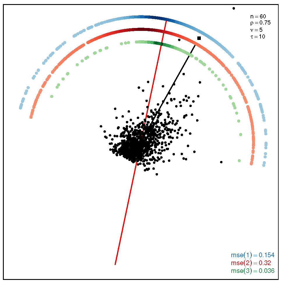
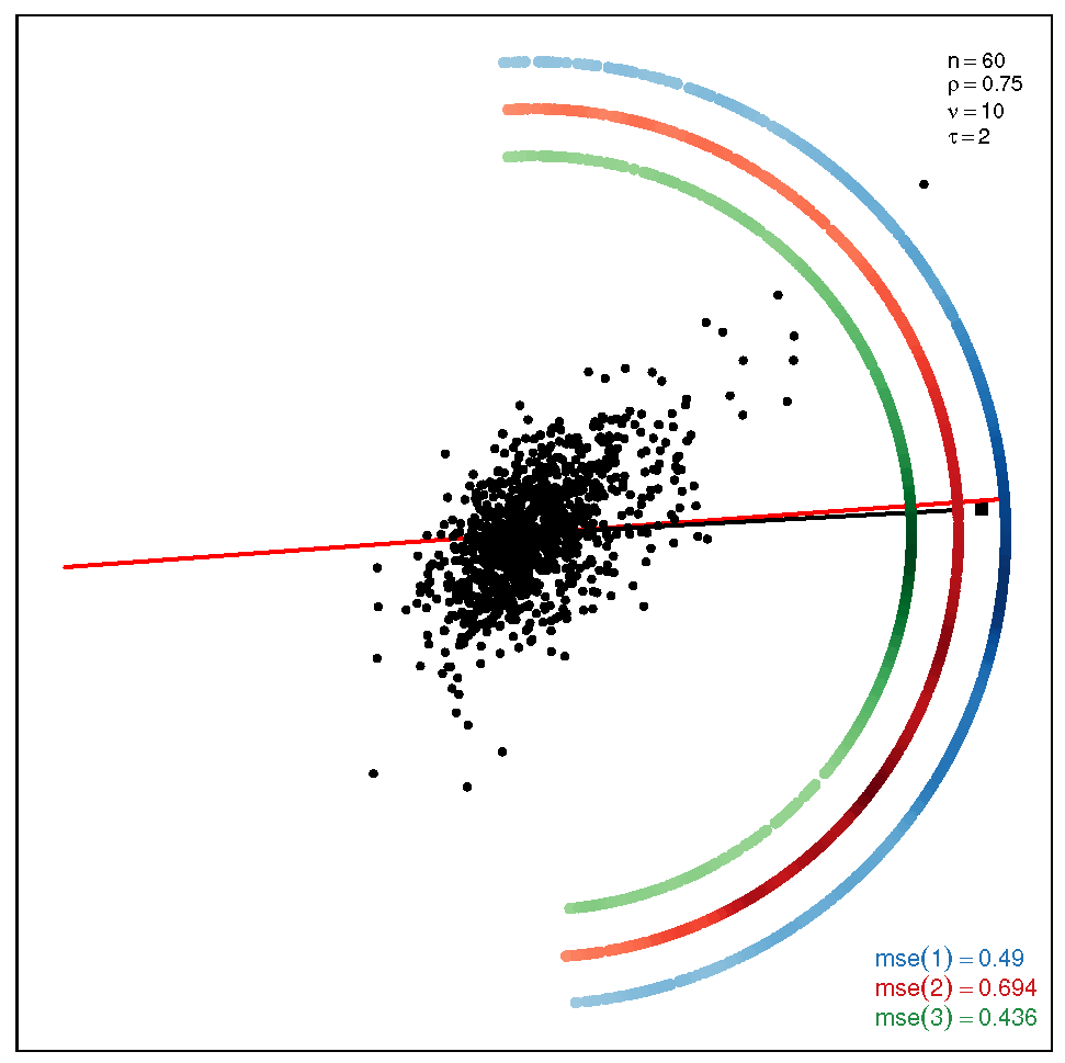
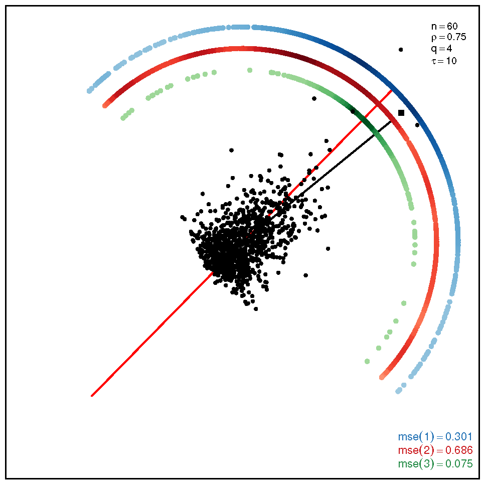
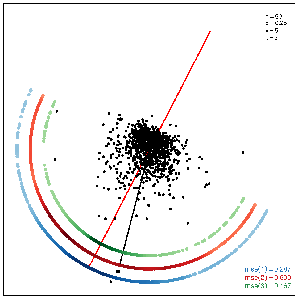
This section addresses the bidimensional case; the outputs of the simulations are summarized by means of plots of directions arranged in tables of figures that display the following information: the red and black lines represent the directions of the theoretical shape vectors $\mathit{\eta }$ and $\mathit{\alpha }$, respectively. On the other hand, the points in the coloured circular crowns correspond to the locations of the directions estimated by the proposed estimation methods, with the blue crown showing the estimations provided by M1, the red crown by M2 and the green crown by M3; their MSE values are displayed at the bottom right legend of each figure. Finally, the clouds of points for the observations obtained by the simulations are also depicted for completeness.

In order to assess the performance of the estimation methods for the bidimensional case, the simulation assays are carried out taking a sample size $n=60$ which may be a representative choice of the small data sets arising in real studies. The plots depicted in

Table 1. Plots with the theoretical and estimated directions under the bidimensional ST distribution when $\rho =0.25$.

	$\tau =2$	$\tau =5$	$\tau =10$
$\nu =5$
$\nu =10$

show the MSEs obtained for samples coming from a ST distribution when $\rho =0.25$. Overall, we can observe that methods M1 and M3 are more accurate than M2. The outputs show that the errors are quite similar for all the methods in the scenario closer to the normal model, provided by the pair $(\tau ,\nu )=(2,10)$; starting from this scenario, we can see that, as we inject asymmetry into the multivariate model, M1 outperforms methods M2 and M3 but its accuracy gets worse when we move to the heavy tail scenarios for $\nu =5$; in such a case, M3 provides the most accurate results ($MSE=0.495,0.167,0.080$). On the other hand, the results displayed by the plots in

Table 2. Plots with the theoretical and estimated directions under the bidimensional ST distribution when $\rho =0.75$.

	$\tau =2$	$\tau =5$	$\tau =10$
$\nu =5$
$\nu =10$

for the coefficient $\rho =0.75$ show that M3 is the most accurate method in all the situations, with its best performance ($MSE=0.036$) in the scenario which is furthest away from the normal distribution.

The results of the simulations under the SSL distribution are given by the plots displayed in

Table 3. Plots with the theoretical and estimated directions under the bidimensional SSL distribution when $\rho =0.25$.

	$\tau =2$	$\tau =5$	$\tau =10$
$q=4$
$q=10$

and

Table 4. Plots with the theoretical and estimated directions under the bidimensional SSL distribution when $\rho =0.75$.

	$\tau =2$	$\tau =5$	$\tau =10$
$q=4$
$q=10$

. In this case, the accuracy of the estimation methods presents similar patterns as those ones observed under the ST model, with the exceptions of the non-normality pair $(\tau ,q)=(10,10)$ at the bottom right corner, where M3 outperforms M1 and M2, and the pair $(\tau ,q)=(2,4)$, at the top right corner, where M2 and M3 are outperformed by M1. When the coefficient $\rho$ is equal to $0.75$ (see Table 4), we can observe once again that M3 gives more accurate results than M1 and M2.

We have deployed additional experiments for other sample sizes, not reported here for the sake of space. In order to illustrate their results, we provide a representative case when $n=200$ for the scenario with the highest asymmetry and tail weight under both multivariate models ST and SSL. The results are displayed by the plots appearing in the figures of

Table 5. Plots with the theoretical and estimated directions under the bidimensional ST (left) and SSL (right) distributions for the highest asymmetry and tail weight levels when $\rho =0.75$.

$(\tau ,\nu )=(10,5)$	$(\tau ,q)=(10,4)$

; they show the remarkably superiority of method M3.

4.2. Simulation Study for SMSN Distributions when $p>2$

We have carried out a wide range of experimental trials for dimensions greater than two. Here, we just provide the results obtained from a few simulation assays—for dimensions $p=4,8$ and sample sizes $n=60,120,240$—which summarize and illustrate our main findings (see

Table 6. Results under the ST distribution. For each non-normality pair $(\tau ,\nu )$, dimensions of the data frame $(p,n)$ and coefficient $\rho$, the cells contain the MSEs given by method 1 (first row), method 2 (second row) and method 3 (third row).

$(\mathit{p},\mathit{n})$	$(4,60)$		$(4,120)$		$(8,120)$		$(8,240)$
$\mathit{\rho }$	$\mathbf{0.25}$	$\mathbf{0.75}$	$\mathbf{0.25}$	$\mathbf{0.75}$	$\mathbf{0.25}$	$\mathbf{0.75}$	$\mathbf{0.25}$	$\mathbf{0.75}$
$(\mathit{\tau },\mathit{\nu })$
$(2,5)$	0.646	0.916	0.500	0.584	1.306	1.090	1.284	1.472
	0.772	0.975	0.677	0.675	1.383	1.155	1.521	1.632
	0.654	0.875	0.435	0.528	1.090	0.931	0.826	0.903
$(2,10)$	0.610	0.932	0.518	0.553	0.873	1.182	1.195	1.280
	0.760	1.075	0.865	0.665	1.029	1.260	1.525	1.580
	0.668	0.831	0.542	0.579	0.938	1.097	0.888	0.838
$(5,5)$	0.258	0.581	0.402	0.403	0.757	1.303	0.634	0.768
	0.443	0.801	0.794	0.629	0.956	1.413	0.971	1.048
	0.338	0.355	0.167	0.105	0.640	0.526	0.244	0.187
$(5,10)$	0.362	0.738	0.299	0.477	0.536	0.918	0.369	0.550
	0.622	1.048	0.769	0.953	0.733	1.157	0.854	1.107
	0.469	0.428	0.198	0.195	0.557	0.785	0.227	0.254
$(10,5)$	0.382	0.496	0.456	0.573	0.696	0.749	0.632	0.944
	0.618	0.725	0.894	0.977	0.938	0.899	0.987	1.263
	0.305	0.333	0.128	0.067	0.550	0.315	0.101	0.107
$(10,10)$	0.495	0.549	0.167	0.644	0.657	0.731	0.265	0.460
	0.776	0.888	0.620	1.165	1.006	0.950	0.837	0.966
	0.426	0.319	0.118	0.179	0.656	0.453	0.145	0.106

and

Table 7. Results under the SSL distribution. For each non-normality pair $(\tau ,q)$, dimensions of the data frame $(p,n)$ and coefficient $\rho$, the cells contain the MSEs given by method 1 (first row), method 2 (second row) and method 3 (third row).

$(\mathit{p},\mathit{n})$	$(4,60)$		$(4,120)$		$(8,120)$		$(8,240)$
$\mathit{\rho }$	$\mathbf{0.25}$	$\mathbf{0.75}$	$\mathbf{0.25}$	$\mathbf{0.75}$	$\mathbf{0.25}$	$\mathbf{0.75}$	$\mathbf{0.25}$	$\mathbf{0.75}$
$(\mathit{\tau },\mathit{q})$
$(2,4)$	0.817	0.854	0.963	1.104	1.406	1.553	0.893	1.528
	0.929	0.900	1.209	1.332	1.491	1.632	1.020	1.652
	0.732	0.796	0.735	0.748	1.144	1.039	0.741	0.933
$(2,10)$	0.739	0.776	0.678	0.843	1.306	1.410	1.039	1.249
	0.851	0.844	1.026	1.279	1.458	1.595	1.423	1.625
	0.852	0.803	0.698	0.604	1.273	1.246	0.956	0.988
$(5,4)$	0.347	0.667	0.225	0.567	1.243	1.510	1.078	1.356
	0.516	0.841	0.462	0.763	1.402	1.634	1.351	1.582
	0.455	0.439	0.232	0.254	0.767	0.676	0.347	0.328
$(5,10)$	0.413	0.650	0.125	0.289	1.057	1.284	0.598	0.738
	0.784	1.005	0.439	0.813	1.455	1.579	1.379	1.516
	0.655	0.648	0.162	0.200	0.804	0.889	0.392	0.293
$(10,4)$	0.383	0.720	0.392	0.463	1.209	1.439	1.104	1.275
	0.574	0.941	0.735	0.830	1.396	1.564	1.420	1.572
	0.401	0.332	0.162	0.103	0.565	0.574	0.260	0.160
$(10,10)$	0.222	0.588	0.163	0.207	0.905	1.202	0.550	0.902
	0.524	1.004	0.657	0.826	1.379	1.598	1.391	1.500
	0.430	0.452	0.318	0.131	0.537	0.775	0.224	0.280

). As could be expected, we observe that, as the dimension increases, the accuracy of all the estimation methods deteriorates, with M3 being the most resistant method to the curse of dimensionality.

Under the ST distribution, the results of Table 6 report the following findings: when $p=4$ and $\rho =0.25$, the estimations given by methods M1 and M3 show similar competitive accuracies provided that $n=60$, whereas the superiority of M3 can be observed for the sample size $n=120$, especially in the case of a heavier tail weight $\nu =5$. When we take $\rho =0.75$, the superiority of M3 becomes more remarkable, as M1 tends to get worse while M3 gains in accuracy, with the lowest MSE appearing when $n=120$ in the furthest scenario from the normal model $(\tau ,\nu )=(10,5)$. When we move to the higher dimension $p=8$, the errors increase to values greater than 1 in many cases, specifically in the scenarios closer to the normality; we can also see that, as the asymmetry and tail weight increase, the accuracy of M1 and M3 improves, with the latter giving acceptable errors ($MSE=0.101,0.107$) at the sample size $n=240$.

For the SSL distribution, the general patterns reported for the case of the ST model come up once again: all the estimation methods give similar accuracies in the scenarios close to normality, M1 and M3 have a good performance as the asymmetry increases, with a better behavior of M3 for the heavier tail weight; note that this pattern becomes more remarkable for the larger coefficient $\rho =0.75$. Nevertheless, in this case, we can observe the negative impact of the dimension on the performance of M1, and particularly M2, methods which in most cases yield very large MSEs. Unlike them, M3 gives very good estimations with the minimum errors ranging in the interval $(0.150,0.300)$.

Finally, we would like to stress that the curse of dimensionality has a smaller impact on the performance of method M3 than some other simulation experiments, not reported here for the sake of space, have shown. Here, we provide an illustrative example: when we consider a ST vector with dimension $p=15$ and parametric settings given by $\rho =0.25$ and $(\tau ,\nu )=(10,5)$, the values of the MSE for the sample size $n=200$ are $1.587$ (M1), $1.684$ (M2) and $0.615$ (M3).

5. Summary and Concluding Remarks

This paper has addressed the skewness-based PP problem when the underlying multivariate distribution of the input vector belongs to the family of SMSN distributions. We have presented skewness PP as an eigenvector problem based on either the third order cumulant matrix or well-known scatter matrices of the model; the connection between the resulting dominant eigenvectors and the shape vector that regulates the asymmetry of the multivariate model has been established, such a connection also sheds light on the interpretability of PP and the ICS method when approached from the parametric framework. The theoretical results point out three methods for estimating the skewness PP direction; the application to artificial data has allowed us to evaluate their performance and has also provided useful insights for comparing them.

This paper has also gone through the role played by the shape vector of the model to assess the multivariate asymmetry in a directional way. However, it is not clear to us how the tail weight and shape vector of the SMSN distribution act together to account for the multivariate non-normality. We conjecture that the issue should be addressed by examining the role of both parameters as indicators of non-normality in accordance to well-defined multivariate stochastic orderings along the lines of previous work [58,59,60]. To the best of the authors’ knowledge, the issue is still unexplored and may deserve future theoretical research to achieve a deeper understanding about their role as non-normality indicators in the SMSN family.

References

1. Kruskal, J.B. Toward a practical method which helps uncover the structure of a set of multivariate observations by finding the linear transformation which optimizes a new “index of condensation”. In Statistical Computation; Elsevier: Amsterdam, The Netherlands, 1969; pp. 427–440. [Google Scholar]
2. Friedman, J.H.; Tukey, J.W. A Projection Pursuit Algorithm for Exploratory Data Analysis. IEEE Trans. Comput. 1974, 23, 881–890. [Google Scholar] [CrossRef]
3. Huber, P.J. Projection Pursuit. Ann. Stat. 1985, 13, 435–475. [Google Scholar] [CrossRef]
4. Jones, M.C.; Sibson, R. What is Projection Pursuit? J. R. Stat. Society. Ser. A 1987, 150, 1–37. [Google Scholar] [CrossRef]
5. Friedman, J.H. Exploratory Projection Pursuit. J. Am. Stat. Assoc. 1987, 82, 249–266. [Google Scholar] [CrossRef]
6. Hall, P. On Polynomial-Based Projection Indices for Exploratory Projection Pursuit. Ann. Stat. 1989, 17, 589–605. [Google Scholar] [CrossRef]
7. Cook, D.; Buja, A.; Cabrera, J. Projection Pursuit Indexes Based on Orthonormal Function Expansions. J. Comput. Graph. Stat. 1993, 2, 225–250. [Google Scholar] [CrossRef]
8. Peña, D.; Prieto, F.J. Cluster Identification Using Projections. J. Am. Stat. Assoc. 2001, 96, 1433–1445. [Google Scholar] [CrossRef] [Green Version]
9. Rodriguez Martinez, E.; Goulermas, J.; Mu, T.; Ralph, J. Automatic Induction of Projection Pursuit Indices. Neural Netw. IEEE Trans. 2010, 21, 1281–1295. [Google Scholar] [CrossRef]
10. Hou, S.; Wentzell, P. Re-centered kurtosis as a projection pursuit index for multivariate data analysis. J. Chemom. 2014, 28, 370–384. [Google Scholar] [CrossRef]
11. Loperfido, N. Skewness-Based Projection Pursuit: A Computational Approach. Comput. Stat. Data Anal. 2018, 120, 42–57. [Google Scholar] [CrossRef]
12. Loperfido, N. Kurtosis-based projection pursuit for outlier detection in financial time series. Eur. J. Financ. 2020, 26, 142–164. [Google Scholar] [CrossRef]
13. Posse, C. Projection pursuit exploratory data analysis. Comput. Stat. Data Anal. 1995, 20, 669–687. [Google Scholar] [CrossRef]
14. De Lathauwer, L.; De Moor, B.; Vandewalle, J. On the best rank-1 and rank-(R1, R2, …, RN) approximation of higher-order tensor. SIAM J. Matrix Anal. Appl. 2000, 21, 1324–1342. [Google Scholar] [CrossRef]
15. Kofidis, E.; Regalia, P.A. On the Best Rank-1 Approximation of Higher-Order Supersymmetric Tensors. SIAM J. Matrix Anal. Appl. 2002, 23, 863–884. [Google Scholar] [CrossRef] [Green Version]
16. Loperfido, N. A new kurtosis matrix, with statistical applications. Linear Algebra Its Appl. 2017, 512, 1–17. [Google Scholar] [CrossRef]
17. Franceschini, C.; Loperfido, N. An Algorithm for Finding Projections with Extreme Kurtosis. In Studies in Theoretical and Applied Statistics; Perna, C., Pratesi, M., Ruiz-Gazen, A., Eds.; Springer: Berlin/Heidelberg, Germany, 2018; pp. 61–70. [Google Scholar]
18. Loperfido, N. Canonical transformations of skew-normal variates. TEST 2010, 19, 146–165. [Google Scholar] [CrossRef]
19. Arevalillo, J.M.; Navarro, H. A note on the direction maximizing skewness in multivariate skew-t vectors. Stat. Probab. Lett. 2015, 96, 328–332. [Google Scholar] [CrossRef]
20. Arevalillo, J.M.; Navarro, H. Skewness-Kurtosis Model-Based Projection Pursuit with Application to Summarizing Gene Expression Data. Mathematics 2021, 9, 954. [Google Scholar] [CrossRef]
21. Kim, H.M.; Kim, C. Moments of scale mixtures of skew-normal distributions and their quadratic forms. Commun. Stat. Theory Methods 2017, 46, 1117–1126. [Google Scholar] [CrossRef]
22. Arevalillo, J.M.; Navarro, H. Data projections by skewness maximization under scale mixtures of skew-normal vectors. Adv. Data Anal. Classif. 2020, 14, 435–461. [Google Scholar] [CrossRef]
23. Capitanio, A. On the canonical form of scale mixtures of skew-normal distributions. Statistica 2020, 80, 145–160. [Google Scholar]
24. Malkovich, J.F.; Afifi, A.A. On Tests for Multivariate Normality. J. Am. Stat. Assoc. 1973, 68, 176–179. [Google Scholar] [CrossRef]
25. Azzalini, A.; Capitanio, A. Statistical applications of the multivariate skew normal distribution. J. R. Stat. Soc. Ser. B 1999, 61, 579–602. [Google Scholar] [CrossRef]
26. Azzalini, A. The Skew-normal Distribution and Related Multivariate Families. Scand. J. Stat. 2005, 32, 159–188. [Google Scholar] [CrossRef]
27. Contreras-Reyes, J.E.; Arellano-Valle, R.B. Kullback–Leibler Divergence Measure for Multivariate Skew-Normal Distributions. Entropy 2012, 14, 1606–1626. [Google Scholar] [CrossRef] [Green Version]
28. Balakrishnan, N.; Scarpa, B. Multivariate measures of skewness for the skew-normal distribution. J. Multivar. Anal. 2012, 104, 73–87. [Google Scholar] [CrossRef]
29. Balakrishnan, N.; Capitanio, A.; Scarpa, B. A test for multivariate skew-normality based on its canonical form. J. Multivar. Anal. 2014, 128, 19–32. [Google Scholar] [CrossRef]
30. Azzalini, A.; Capitanio, A. The Skew-Normal and Related Families; IMS Monographs; Cambridge University Press: Cambridge, UK, 2014. [Google Scholar]
31. González-Farías, G.; Domínguez-Molina, A.; Gupta, A.K. Additive properties of skew normal random vectors. J. Stat. Plan. Inference 2004, 126, 521–534. [Google Scholar] [CrossRef]
32. González-Farías, G.; Domínguez-Molina, A.; Gupta, A.K. The closed skew-normal distribution. In Skew-Elliptical Distributions and Their Applications: A Journey Beyond Normality; Genton, M.G., Ed.; Chapman & Hall/CRC: Boca Raton, FL, USA, 2004; Chapter 2; pp. 25–42. [Google Scholar]
33. Loperfido, N. Generalized skew-normal distributions. In Skew-Elliptical Distributions and Their Applications: A Journey Beyond Normality; Genton, M.G., Ed.; Chapman & Hall/CRC: Boca Raton, FL, USA, 2004; Chapter 4; pp. 65–80. [Google Scholar]
34. Lachos, V.H.; Labra, F.V.; Bolfarine, H.; Ghosh, P. Multivariate measurement error models based on scale mixtures of the skew–normal distribution. Statistics 2010, 44, 541–556. [Google Scholar] [CrossRef]
35. Vilca, F.; Balakrishnan, N.; Zeller, C.B. Multivariate Skew-Normal Generalized Hyperbolic distribution and its properties. J. Multivar. Anal. 2014, 128, 73–85. [Google Scholar] [CrossRef]
36. Kahrari, F.; Rezaei, M.; Yousefzadeh, F.; Arellano-Valle, R. On the multivariate skew-normal-Cauchy distribution. Stat. Probab. Lett. 2016, 117, 80–88. [Google Scholar] [CrossRef]
37. Kahrari, F.; Arellano-Valle, R.; Rezaei, M.; Yousefzadeh, F. Scale mixtures of skew-normal-Cauchy distributions. Stat. Probab. Lett. 2017, 126, 1–6. [Google Scholar] [CrossRef]
38. Arellano-Valle, R.B.; Ferreira, C.S.; Genton, M.G. Scale and shape mixtures of multivariate skew-normal distributions. J. Multivar. Anal. 2018, 166, 98–110. [Google Scholar] [CrossRef] [Green Version]
39. Ogasawara, H. A non-recursive formula for various moments of the multivariate normal distribution with sectional truncation. J. Multivar. Anal. 2021, 183, 104729. [Google Scholar] [CrossRef]
40. Azzalini, A.; Dalla Valle, A. The multivariate skew-normal distribution. Biometrika 1996, 83, 715–726. [Google Scholar] [CrossRef]
41. Branco, M.D.; Dey, D.K. A General Class of Multivariate Skew-Elliptical Distributions. J. Multivar. Anal. 2001, 79, 99–113. [Google Scholar] [CrossRef] [Green Version]
42. Kim, H.M. A note on scale mixtures of skew normal distribution. Stat. Probab. Lett. 2008, 78, 1694–1701. [Google Scholar] [CrossRef]
43. Basso, R.M.; Lachos, V.H.; Cabral, C.R.B.; Ghosh, P. Robust mixture modeling based on scale mixtures of skew-normal distributions. Comput. Stat. Data Anal. 2010, 54, 2926–2941. [Google Scholar] [CrossRef]
44. Zeller, C.B.; Cabral, C.R.B.; Lachos, V.H. Robust mixture regression modeling based on scale mixtures of skew-normal distributions. TEST 2016, 25, 375–396. [Google Scholar] [CrossRef]
45. Lachos, V.H.; Garay, A.M.; Cabral, C.R.B. Moments of truncated scale mixtures of skew-normal distributions. Braz. J. Probab. Stat. 2020, 34, 478–494. [Google Scholar] [CrossRef]
46. Azzalini, A.; Capitanio, A. Distributions generated by perturbation of symmetry with emphasis on a multivariate skew t-distribution. J. R. Stat. Soc. Ser. B 2003, 65, 367–389. [Google Scholar] [CrossRef]
47. Wang, J.; Genton, M.G. The multivariate skew-slash distribution. J. Stat. Plan. Inference 2006, 136, 209–220. [Google Scholar] [CrossRef]
48. Loperfido, N. Skewness and the linear discriminant function. Stat. Probab. Lett. 2013, 83, 93–99. [Google Scholar] [CrossRef]
49. Kollo, T.; von Rosen, D. Advanced Multivariate Statistics with Matrices; Mathematics and Its Applications; Springer: Dordrecht, The Netherlands, 2005. [Google Scholar]
50. Christiansen, M.C.; Loperfido, N. Improved Approximation of the Sum of Random Vectors by the Skew Normal Distribution. J. Appl. Probab. 2014, 51, 466–482. [Google Scholar] [CrossRef]
51. Qi, L. Rank and eigenvalues of a supersymmetric tensor, the multivariate homogeneous polynomial and the algebraic hypersurface it defines. J. Symb. Comput. 2006, 41, 1309–1327. [Google Scholar] [CrossRef] [Green Version]
52. Cardoso, J.F. Source separation using higher order moments. In Proceedings of the International Conference on Acoustics, Speech, and Signal Processing, Glasgow, UK, 23–26 May 1989; pp. 2109–2112. [Google Scholar]
53. Tyler, D.E.; Critchley, F.; Dümbgen, L.; Oja, H. Invariant co-ordinate selection. J. R. Stat. Soc. Ser. B 2009, 71, 549–592. [Google Scholar] [CrossRef]
54. Kent, J.T. Discussion on the paper by Tyler, Critchley, Dumbgen & Oja: Invariant co-ordinate selection. J. R. Stat. Soc. Ser. B 2009, 71, 575–576. [Google Scholar]
55. Peña, D.; Prieto, F.J.; Viladomat, J. Eigenvectors of a kurtosis matrix as interesting directions to reveal cluster structure. J. Multivar. Anal. 2010, 101, 1995–2007. [Google Scholar] [CrossRef] [Green Version]
56. Alashwali, F.; Kent, J.T. The use of a common location measure in the invariant coordinate selection and projection pursuit. J. Multivar. Anal. 2016, 152, 145–161. [Google Scholar] [CrossRef] [Green Version]
57. Nordhausen, K.; Oja, H.; Tyler, D.E. Tools for Exploring Multivariate Data: The Package ICS. J. Stat. Softw. 2008, 28, 1–31. [Google Scholar] [CrossRef]
58. Wang, J. A family of kurtosis orderings for multivariate distributions. J. Multivar. Anal. 2009, 100, 509–517. [Google Scholar] [CrossRef] [Green Version]
59. Arevalillo, J.M.; Navarro, H. A study of the effect of kurtosis on discriminant analysis under elliptical populations. J. Multivar. Anal. 2012, 107, 53–63. [Google Scholar] [CrossRef] [Green Version]
60. Arevalillo, J.M.; Navarro, H. A stochastic ordering based on the canonical transformation of skew-normal vectors. TEST 2019, 28, 475–498. [Google Scholar] [CrossRef]