A Statistical Analysis of Observational Hubble Parameter Data to Discuss the Cosmology of Holographic Chaplygin Gas

Abstract

A scheme for the generalized Chaplygin gas equation of state is shown by using the holographic Ricci dark energy. Regression analysis and a chi-square test were performed. A second order polynomial regression has been established as the relation between the Hubble Parameter and redshift. It has established a set of parameters that can predict the Equation of State (EoS) parameter.

1. Introduction

It is well documented in the literature that our universe is going through a phase of late time acceleration [1,2,3,4,5,6,7,8,9]. In order to explain this late time acceleration, we require a driving force. An exotic matter that is considered to be responsible for this late time acceleration is referred to as Dark Energy (DE) [10,11,12]. DE is currently a mystery of modern cosmology. Its exact behavior is yet to be fully understood. For a detailed review of DE see. The cosmological constant is considered to be the simplest candidate of DE. In this context, it may be noted that DE is characterized by a negative Equation of State (EoS) parameter $w=p/\rho$, where p and $\rho$ denote the pressure and energy density of the universe, respectively. In order for the acceleration to exist, one requires w to be less than $-1/3$. The line $w=-1$ is considered to be the phantom boundary. If for some model $w>-1$ then it is called quintessence and if $w\le -1$ then it is called phantom. If the EoS w for a model gets a transition from quintessence to phantom then it is considered to be a quintom model for cosmological constant $w=-1$. Although the cosmological constant is supported by observations, models with a time varying EoS parameter have also been considered in a lot of the literature. Such kinds of DE models can be broadly categorized into: (i) Scalar field models, (ii) holographic models, and (iii) Chaplygin gas models. The present work intends to statistically explore a reconstruction scheme for generalized Chaplygin gas (GCG) through Holographic Ricci Dark Energy (HRDE) under the preview of regression and hypothesis testing. In this context, let us mention about some important works on GCG. Using the available cosmological data, authors of [13] put constraints on the free parameters of the new GCG model based on the statistical Markov chain Monte Carlo method. Reference [14] considered an interaction between cold dark matter and GCG and constrained the model parameter $\alpha$. Reference [15] demonstrated an interacting scenario between GCG and dark matter under the purview of bulk viscosity in $f(R,T)$ gravity framework. In view of these studies, we have decided to look into a reconstruction scheme of GCG under holographic setting and through the method of hypothesis testing.

Since the present work contemplates to investigate DE candidates, namely GCG and HRDE, we need to have a look at the relevant literature. CG is a modified matter categorized from the dynamical dark energy model. In general the equation of state representing CG is given by, $p=-B/\rho$, where p is the pressure and $\rho$ is the energy density of the fluid and B is a positive constant. Different extended versions of CG have been studied in the literature as a DE candidate to interpret the accelerated expansion of the universe. One interesting property of different versions of CG is that it can unify the early and later stages of the universe. A generalized version of CG as GCG was proposed in several references [16,17]. An exotic equation of generalized Chaplygin gas (GCG) has been deduced as $p=-B/{\rho }^{\alpha }$, where an additional parameter $\alpha$ is introduced. The model parameter $\alpha$ can take on values $0<\alpha \le 1$. In order to perceive more accurate result the equation of modified CG (MCG) has been introduced as $p=A\rho -B/{\rho }^{\alpha }$, where A and B are positive constants. A modification was proposed for considering A and B as a function of scale factor $a\left(t\right)$.

A model of DE, which is also known as modified holographic Ricci dark energy (HRDE), is a function of the Hubble parameter and the first derivative with respect to cosmic time t [18]. HRDE manifests quintom features. The main characteristic of HRDE is governed by a positive numerical parameter $\alpha$ in the model. This $\alpha$ plays an important role in determining the evolutionary behavior of the DE. When $\alpha <1/2$, the HRDE will exhibit a quintom like behavior i.e., its equation of state will evolve across the cosmological constant boundary $w=-1$ [19]. Observations show that the parameter $\alpha$ is indeed smaller than $1/2$, so the late time evolution of RDE will be really like a phantom energy.

In certain cases, the cosmic coincidence problem comes in the way of parameters of a quintessence model, so inevitably this model fails to adjust very precisely with certain observations. This problem demonstrates the reason behind the fact that the vacuum energy or scalar field dominate the universe for late time acceleration. This problem is addressed by quintessence models through the evolution of quintessence energy density, which does not depend on the initial condition. Nevertheless, a fine-tuning of potential parameters is required in order to make changes in the behavior of quintessence energy density at epoch of the equality of matter-radiation. This has finally resulted in domination of dark energy over dark matter leading to late time acceleration of the universe [20,21].

Phantom cosmology is characterized by a kind of future singularity called the ‘big rip’ [22]. In this context [23] modeled the augmentation of phantom dark energy onto a black hole. The former study showcased, due to strong negative pressure of phantom energy the black hole mass will gradually decrease and tend to zero near the big rip where it will finally disappear. Later studies [24] have shown the dominance of quantum effects near the big rip and as the consequence the mass of black hole is reduced to a finite value. Another study [19] has established that there is a possibility of an increase in the mass of a black hole due to accretion onto which [25].

In the present work we endeavor to generate a reconstruction scheme for generalized Chaplygin gas EoS with the aim of establishing the relation between the GCG and HRDE. The regression based method is adopted and the goodness-of-fit is tested to ${\chi }^2$. The rest of the paper is organized as follows: in Section 2 we have fitted the regression equation with redshift z as the predictor and Hubble parameter H as the predictand. In the next phase, i.e., in Section 3, we have considered the generalized Chaplygin gas under the purview of HRDE and accordingly carried out ${\chi }^2$ test for establishing goodness-of-fit of the prediction model for H. We have concluded in Section 4.

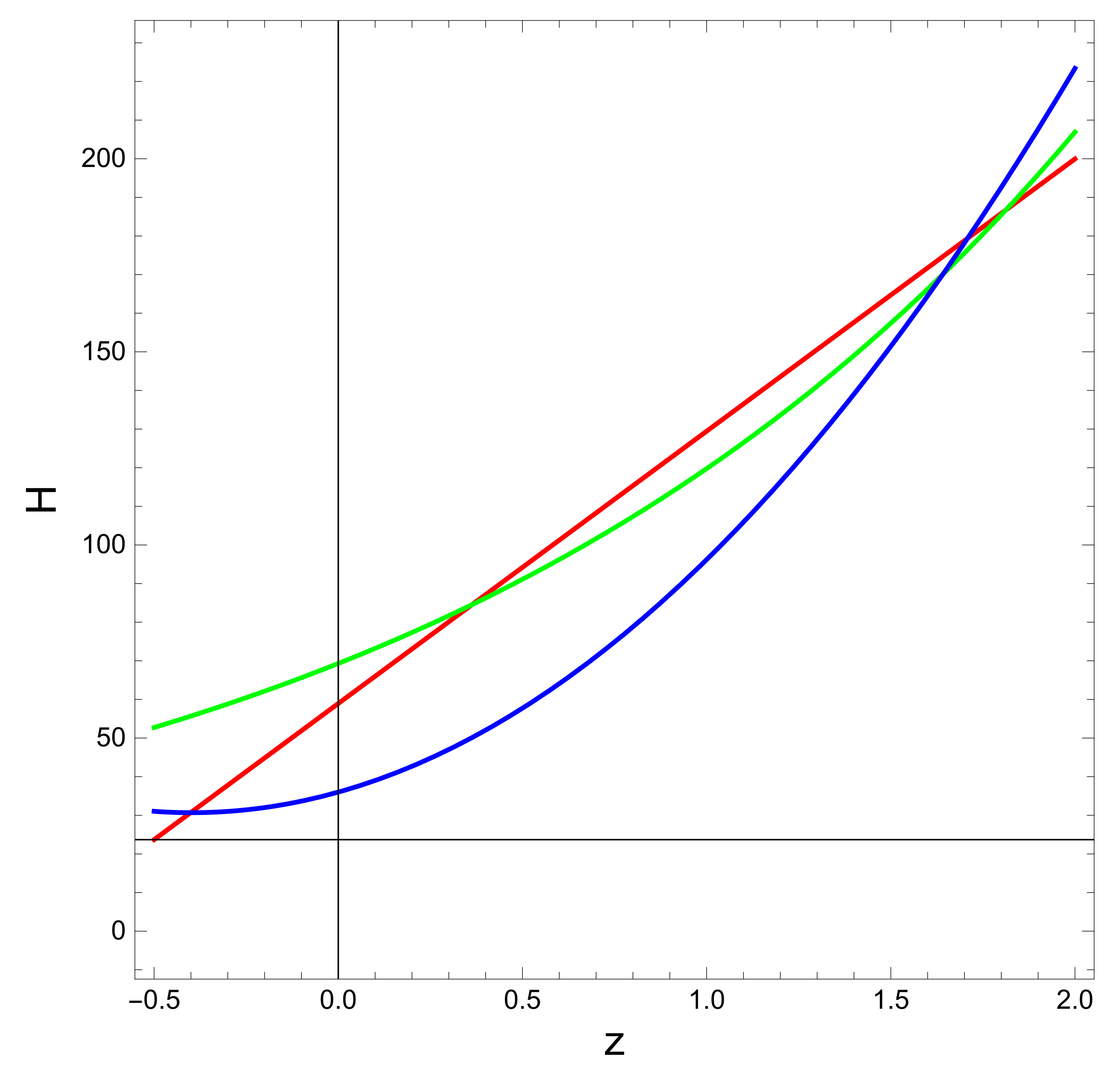
2. Fitting Regression Equation to the Observational Data

In this section we develop a regression equation with redshift z as a predictor and Hubble parameter H as the predictand. A regression equation basically describes the relationship between two variables and in the present study we consider linear as well as nonlinear regression equation. The regression constants and coefficients are determined by the method of least squares [26]. For sake of deriving a suitable functional relation between z and H, we need to find the best possible Regression relation between them. To evaluate the best fit we will calculate $R^2$, where $R^2=\frac{SSR}{SST}$. The term SST is an acronym for sum of squares total, which mathematically implies the sum of square deviations of the value of the dependent variables around their mean. SSR stands for the regression sum of squares and mathematically it implies the sum of square differences between the regression predictions and the sample mean of the predictand. Details of regression method are available in [26]. Among the regression relations, whichever gives the highest value of $R^2$ close to 1, will be considered as the best model. We have tried three models,

$$\begin{array}{c}\hfill H=b_0+b_{1}z\end{array}$$

(1)

$$\begin{array}{c}\hfill H=b_0{e}^{\left(b_{1}z\right)}\end{array}$$

(2)

$$\begin{array}{c}\hfill H=b_0+b_{1}z+b_2{z}^2\end{array}$$

(3)

In the above equations, H and z represent the Hubble parameter and redshift, respectively. Furthermore, $b_0$ represents regression constant and $b_1,b_2$ are the regression coefficients of the respective models. The three models of regression represented by Equations (1)–(3) are now fit to the data presented in

Table 1. Hubble parameter data [27].

z	H (z) (km/s/Mpc)
0.07	69
0.09	69
0.12	68.6
0.17	83
0.179	75
0.199	75
0.2	72.9
0.27	77
0.28	88.8
0.352	83
0.38	81.9
0.3802	83
0.4	95
0.4004	77
0.4247	87.1
0.4497	92.8
0.47	89
0.4783	80.9
0.48	97
0.52	90.8
0.593	104
0.61	97.8
0.68	92
0.781	105
0.875	125
0.88	90
0.9	117
1.037	154
1.3	168
1.363	160
1.43	177
1.53	140
1.75	202
1.965	186.5
2.34	223
2.36	227

and the corresponding $R^2$ is evaluated for each model. The outcomes are presented in

Table 2. The three regression models and the corresponding $R^2$.

Regression Model	${\mathit{R}}^{\mathbf{2}}$
$H=b_0+b_{1}z$	0.9394
$H=b_0{e}^{\left(b_{1}z\right)}$	0.9246
$H=b_0+b_{1}z+b_2{z}^2$	0.9404

.

Considering the highest value of $R^2$, the third model i.e., $H=b_0+b_{1}z+b_2{z}^2$ is considered to be the best model to establish the functional relationship between z and $H\left(z\right)$. In this context we would like to mention that the three regression equations considered here are linear, exponential, and polynomial types, respectively. These are three important forms of regression and in all the cases the regression coefficients and the regression constants have been determined through the method of least squares, where the sum squares of the errors is minimized by taking partial derivatives with respect to regression coefficients and constants and then equating to zero. These approaches have been adopted here, and accordingly, the regression coefficients and constants have been determined. All the models have been proved to be almost equally efficient through the high value of $R^2$. Four decimal places have been retained to understand the relative efficiency of the model. Although the three models have equal efficiency, the model represented by Equation (3) is found to be more accurate than Equations (1) and (2) and hence considered for subsequent study. We would like to point out that in Table 1 we have considered the Hubble parameter data available in [27], where there are some associated errors. In the present work, we intend to generate a regression-based methodology for correspondence between the generalized Chaplygin gas (GCG) and holographic Ricci dark energy (HRDE), which is why we have taken the values and discarded the ± part. This gives the midpoint of the acceptable range of H for the corresponding z and hence does not violate the acceptable range.

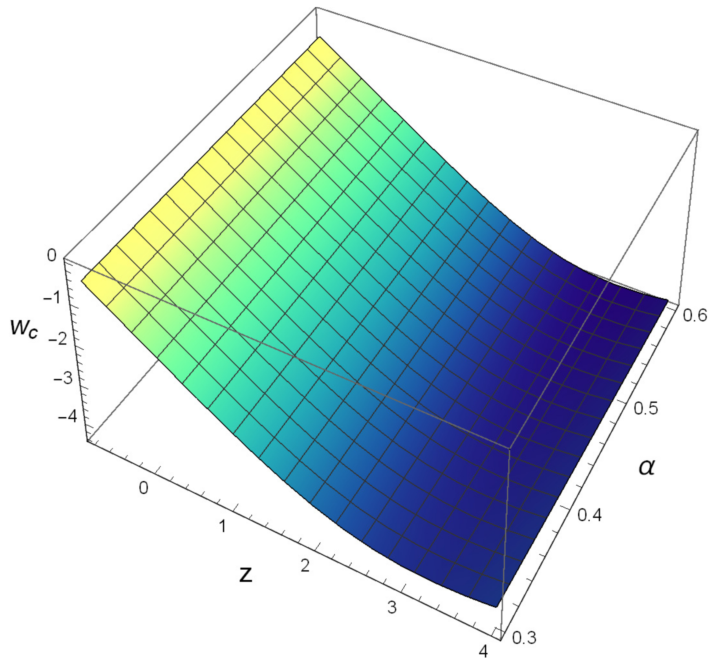
3. Generalized Chaplygin Gas (GCG) in Holographic Ricci Dark Energy (HRDE) Framework

In this section we consider a correspondence between GCG and HRDE. The HRDE is a specific form of more generalized Holographic dark energy Nojiri–Odinsov cut-off [28]. The density of HRDE is given by [18]

$${\rho }_{\mathit{\lambda }}=3c^2\left(\dot{H}+2H^2\right),0<c^2<1$$

(4)

and the GCG is represented by the equation of state [20]

$$p_c=-\left(\frac{B}{{\rho }_c^{\alpha }}\right)$$

(5)

that implies

$${\rho }_c={\left(-\frac{B}{p_c}\right)}^{\frac{1}{\alpha }}$$

(6)

where $p_c$ and ${\rho }_c$ represent the pressure and density respectively for GCG, $0<\alpha <1$ and H is the Hubble parameter. Constraints on B and $\alpha$ are already stated in the previous section. Hence the EoS parameter $w_c$ of GCG takes the form

$$w_c=-\frac{B}{{\rho }_c^{1+\alpha }}$$

(7)

As we are considering a correspondence between GCG and HRDE, we have ${\rho }_{\gamma }={\rho }_c$. From this consideration we have

$$p_c=-\frac{B}{{\left[3c^2(\dot{H}+2H^2)\right]}^{\alpha }}$$

(8)

Based on the equation of state parameter

$$w_c=\frac{p_c}{{\rho }_c}$$

(9)

we intend to express $w_c$ in terms of H(Hubble parameter) and its derivatives. The relations considered here are $3H^2=\rho$ and $\dot{a}=aH$. Subsequently we have

$$\ddot{a}=a\dot{H}+H\dot{a}$$

(10)

and when this is considered in

$$6\frac{\ddot{a}}{a}=-({\rho }_c+3p_c)$$

(11)

and

$$\ddot{a}=a\dot{H}+H\dot{a}$$

(12)

we obtain

$$w_c=-\left(1+\frac{2\dot{H}}{3H^2}\right)$$

(13)

where, $H^2$ is obtained from observational data presented in Table 1. For $\dot{H}$ we consider $\dot{H}=-\frac{1}{{(1+z)}^3}\frac{dH}{dz}$. The $\frac{dH}{dz}$ is computed from the best fit regression equation. If we consider the limiting case $z\to -1$ we get from Equation (3) that $w_c\to -1$. Thus, in the very late stage, the EoS parameter tends to be $-1$. However, the limiting case does not give us any possibility of exit from $-1$ boundary.

Using the first Friedmann equation we have $3H^2={\rho }_{\mathit{\lambda }}$, which leads to the solution for scale factor as

$$a\left(t\right)={\left(\frac{\left(-1+2c^2\right)(C_1+C_{2}t)}{c^2}\right)}^{\frac{c^2}{-1+2c^2}}$$

(14)

Equation (14) represents the scale factor reconstructed under the purview of HRDE. Now we consider the conservation equation for GCG:

$$\dot{{\rho }_c}+3H{\rho }_c\left(1-\frac{B}{{\rho }_c^{1+\alpha }}\right)=0$$

(15)

Solution for the differential Equation (15) gives us reconstructed GCG density as a function of the scale factor a as:

$${\rho }_{c,reconstructed}\left(a\right)={\left(1+a^{-3(1+\alpha )}{e}^{(1+\alpha )C_3}\right)}^{\frac{1}{1+\alpha }}$$

(16)

Using Equation (14) in (16) we get the HRDE reconstructed GCG as

$${\rho }_{c,reconstructed}={\left(1+e^{C_3(1+\alpha )}{\left({\left(\frac{\left(-1+2c^2\right)(C_2+C_{1}t)}{c^2}\right)}^{\frac{c^2}{-1+2c^2}}\right)}^{-3(1+\alpha )}\right)}^{\frac{1}{1+\alpha }}$$

(17)

Using Equation (14) in the equation $a=\frac{1}{1+z}$ we can get cosmic time t in terms of redshift z as

$$t=-\frac{C_2+\frac{c^2{(1+z)}^{2-\frac{1}{c^2}}}{1-2c^2}}{C_1}$$

(18)

Using Equation (18) in (16) we can rewrite the HRDE reconstructed GCG density in therm of z as

$${\rho }_{c,reconstructed}={\left(1+e^{C_3(1+\alpha )}{\left({\left({(1+z)}^{2-\frac{1}{c^2}}\right)}^{\frac{c^2}{-1+2c^2}}\right)}^{-3(1+\alpha )}\right)}^{\frac{1}{1+\alpha }}$$

(19)

The HRDE reconstructed GCG density is used in Equation (3) through $3H^2={\rho }_{c,reconstructed}$ and the $\dot{H}$ is obtained from the regression equation already obtained. This reconstructed EoS parameter is plotted in Figure 1 for a range of values of $\alpha$ and it is observed that for the current universe i.e., $z=0$, the reconstructed EoS parameter is close to $-1$ and the EoS is behaving like a phantom. Furthermore, at a later stage, an exit from $-1$ boundary is possible and this indicates termination of phantom-dominated phase of the universe. Also, we have observed that for higher values of $\alpha$, the EoS parameter has a higher slope and reaches the phantom boundary a bit earlier than the lower values.

4. Concluding Remarks and Future Developments

The study reported in the previous sections involves a rigorous statistical analysis of observational Hubble parameter data to understand the cosmology of Chaplygin gas reconstructed though holographic Ricci dark energy. As the first step we have attempted to derive a suitable functional relation between Hubble Parameter H and redshift z. In order to do the same we have tried three regression equations with H as the dependent variable and z as the independent variable. The three forms of regression involved in this study are linear, exponential, and second order polynomial, respectively. After deriving the regression coefficients and constants by the method of least squares, we have computed the coefficients of determination $R^2$ for all the three models. Although we get $R^2>0.9$ for all the three models, the second order polynomial is found to produce the maximum $R^2$. Hence the best fit functional relationship comes out to be $H=b_0+b_{1}z+b_2{z}^2$ where $b_0=36,b_1=26.6973,b_2=33.4992$. It may please be noted that $b_0$, $b_1$, and $b_2$ are determined by the method of least squares. Details of the method are elaborated in [26].

In the next phase of the study we shall consider the Hubble parameter value based on the established functional relationship mentioned above. In this phase we consider a correspondence between GCG and HRDE. From GCG, we obtain the form of EoS parameter $w_c$, which is equated to the reconstructed EoS parameter obtained by considering a correspondence between the density of HRDE and GCG. In this new form of EoS parameter we have the parameters $c,\alpha$ and constant B to be determined.

To further proceed we consider the Friedmann’s Equation $3H^2=\rho$ and this leads to a differential equation giving a general form of pressure as, $p=-3H^2-2\dot{H}$. As a natural consequence we get $w=-\left(1+\frac{2\dot{H}}{3H^2}\right)$. As H has been established as the function of z we can easily calculate $\dot{H}=aH\frac{dH}{dz}\frac{dz}{da}$, where we have the well known relation $a=1/(1+z)$.

We carried out the ${\chi }^2$ test to understand the goodness-of-fit of the EoS parameter via a holographically reconstructed GCG. Here, the form of EoS mentioned above is considered as the observed value and the EoS parameter obtained by the reconstruction scheme as the predicted value. By testing ${\chi }^2$ based on the null hypothesis is of goodness-of-fit, we have carried out the ${\chi }^2$ test for ten sets of values of parameters as reported in

Table 3. Results on the observed and predicted Equation of State (EoS). Parameters $c,\alpha ,\mathrm{and}B$ are for holographic Ricci Chaplygin gas. The $PCC$ stands for Pearson correlation coefficient between observed and predicted Equation of State (EoS) parameter. The tabular values with appropriate degrees of freedom are $22.465$ (at $5\%$), $18.509$ (at $10\%$) and $22.797$ (at $1\%$).

Cases	PCC	${\mathit{R}}^{\mathbf{2}}$	${\mathit{\chi }}_{\mathit{comp}}^{\mathbf{2}}$	Conclusion on ${\mathit{H}}_{\mathbf{0}}$
c = 0.45, $\alpha =0.4$, B = 106	0.531	0.282	22.933	Accepted at $10\%$ level
c = 0.45, $\alpha =0.8$, B = 108	0.528	0.278	68.399	Not accepted
c = 0.45, $\alpha =1.0$, B = 109	0.524	0.274	118.481	Not accepted
c = 0.50, $\alpha =0.4$, B = 106	0.531	0.282	17.146	Accepted at all levels
c = 0.50, $\alpha =0.8$, B = 108	0.528	0.278	46.843	Not accepted
c = 0.50, $\alpha =1.0$, B = 109	0.524	0.275	77.761	Not accepted
c = 0.75, $\alpha =0.4$, B = 107	0.531	0.282	54.615	Not accepted
c = 0.75, $\alpha =0.8$, B = 109	0.528	0.278	108.695	Not accepted
c = 0.75, $\alpha =1.0$, B = 1010	0.524	0.275	153.534	Not accepted

. It may be noted that for all the ten cases the Pearson correlation coefficient comes out to be greater than 0.5. Comparing the computed ${\chi }^2$ with tabular values at $5\%$, $10\%$, and $1\%$ levels of significance. It is observed that the reconstructed model fits best to the observational data for $c=0.5,\alpha =0.4$ and $B=106$. Hence we conclude that it is possible to create an EoS parameter for the GCG reconstructed through HRDE that can fit well to the observational data. At this juncture, it may be noted that for choice of $\alpha$, we have followed the study by Zhang [29], where it was shown that for $\alpha <\frac{1}{2}$, the HRDE has an equation of state parameter behaving like a quintom i.e., it transitions from quintessence to phantom. Following the study of [29], we have chosen $\alpha$ to be in the vicinity of $\frac{1}{2}$ and carried out the hypothesis testing accordingly.

In Figure 2 we have plotted the Hubble parameter H against redshift z for the best fit regression model $H=b_0+b_{1}z+b_2{z}^2$ with the values of the coefficients $b_1=26.6973$$b_2=33.4992$ and $b_0=36$. We have observed that the evolution of the predicted H is showing a decreasing pattern with z. In Figure 1 we have a pictorial representation of the reconstructed EoS parameter $w_c$ for a range of values of $\alpha$ with $B=106$ and $c=0.5$ as both values have been identified through ${\chi }^2$ test in Table 3. It has been observed in this figure that the reconstructed $w_c\approx -1$ at $z=0$ i.e., for the current universe. Hence we can conclude that the model through reconstruction of H through regression is consistent with observation. It is further observed that the reconstructed $w_c$ is staying below $-1$ and crossing the phantom boundary after the evolution passes $z=0$. Hence we can say that the reconstructed $w_c$ has the possibility of crossing the phantom boundary at a later stage of the universe. We propose further studies to examine whether we can have state finder trajectories derived through regression equations to check whether the aforementioned model can have a significant departure from $\mathsf{\Lambda }$CDM. In the context of the studies of [30,31,32] we should comment on the comparison of our model with $\mathsf{\Lambda }$CDM. From the expression of HRDE reconstructed GCG it is apparent that as $z\to -1$, the density becomes asymptotic. This behavior indicates that under this formulation, even without cosmological constant, we can reproduce $\mathsf{\Lambda }$CDM cosmology.

One important point to make for future work worth being mentioned here is that Markov chain Monte Carlo (MCMC) techniques are now widely used for cosmological parameter estimation [33]. The current study primarily focuses on hypothesis testing that involves the chi-square test. The regression parameters have been estimated through the least square method. The MCMC that involves the generation of chains to sample the posterior probability distribution obtained following a Bayesian approach can be effective in estimation of model parameters associated with HRDE reconstructed GCG model. An extension of this current approach is proposed as future study.

At this juncture let us make some remarks: given the recent discovery of gravitational waves [34,35,36]. Ni [34] demonstrated the determination of DE equation, and probing the inflationary physics using space gravitational wave detectors. Figure 1 shows agreement of the results presented in [34]. This figure shows that for the current universe, $w\le -0.9$; this is consistent with the results presented in [34] based on ASTROD-GW mission.

References

1. Amendola, L. Dark Energy: Theory and Observations; Reprint edition; Cambridge University Press: Cambridge, UK, 2015. [Google Scholar]
2. Riess, A.G.; Filippenko, A.V.; Challis, P.; Clocchiatti, A.; Diercks, A.; Garnavich, P.M.; Gilliland, R.L.; Hogan, C.J.; Jha, S.; Kirshner, R.P.; et al. Observational Evidence from Supernovae for an Accelerating Universe and a Cosmological Constant. Astron. J. 1998, 116, 1009. [Google Scholar] [CrossRef] [Green Version]
3. Perlmutter, S.; Aldering, G.; Goldhaber, G.; Knop, R.A.; Nugent, P.; Castro, P.G.; Deustua, S.; Fabbro, S.; Goobar, A.; Groom, D.E.; et al. Measurements of Ω and Λ from 42 High-Redshift Supernovae. Astrophys. J. 1999, 517, 565. [Google Scholar] [CrossRef]
4. Astier, P.; Guy, J.; Regnault, N.; Pain, R.; Aubourg, E.; Balam, D.; Basa, S.; Carlberg, R.G.; Fabbro, S.; Fouchez, D.; et al. The Supernova Legacy Survey: Measurement of ΩM, ΩΛ and w from the first year data set. Astron. Astrophys. 2006, 447, 31. [Google Scholar] [CrossRef] [Green Version]
5. Tegmark, M.; Strauss, M.; Blanton, M.; Abazajian, K.; Dodelson, S.; Sandvik, H.; Wang, X.; Weinberg, D.; Zehavi, I.; Bahcall, N.; et al. Cosmological parameters from SDSS and WMAP. Phys. Rev. D 2004, 69, 103501. [Google Scholar] [CrossRef] [Green Version]
6. Abazajian, K.; Adelman-McCarthy, J.K.; Agueros, M.A.; Allam, S.S.; Anderson, K.S.J.; Anderson, S.F.; Annis, J.; Bahcall, N.A.; Baldry, I.K.; Bastian, S.; et al. The Second Data Release of the Sloan Digital Sky Survey. Astron. J. 2004, 128, 502. [Google Scholar] [CrossRef] [Green Version]
7. Abazajian, K.; Adelman-McCarthy, J.K.; Agueros, M.A.; Allam, S.S.; Anderson, K.S.J.; Anderson, S.F.; Annis, J.; Bahcall, N.A.; Baldry, I.K.; Bastian, S.; et al. The third data release of the sloan digital sky survey. Astron. J. 2005, 129, 1755. [Google Scholar] [CrossRef]
8. Spergel, D.N.; Verde, L.; Peiris, H.V.; Komatsu, E.; Nolta, M.R.; Bennett, C.L.; Halpern, M.; Hinshaw, G.; Jarosik, N.; Kogut, A.; et al. First Year Wilkinson Microwave Anisotropy Probe (WMAP) Observations: Determination of Cosmological Parameters. Astrophys. J. Suppl. 2003, 148, 175. [Google Scholar] [CrossRef] [Green Version]
9. Spergel, D.N.; Bean, R.; Dore, O.; Nolta, M.R.; Bennett, C.L.; Dunkley, J.; Hinshaw, G.; Jarosik, N.; Komatsu, E.; Page, L.; et al. Three-Year Wilkinson Microwave Anisotropy Probe (WMAP) Observations: Implications for Cosmology. Astrophys. J. Suppl. 2007, 170, 377. [Google Scholar] [CrossRef] [Green Version]
10. Padmanabhan, T. Cosmological Constant—The Weight of the Vacuum. Phys. Rep. 2003, 380, 235. [Google Scholar] [CrossRef] [Green Version]
11. Peebles, P.J.E.; Ratra, B. The cosmological constant and dark energy. Rev. Mod. Phys. 2003, 75, 559. [Google Scholar] [CrossRef] [Green Version]
12. Copeland, E.J.; Sami, M.; Tsujikawa, S. Dynamics of dark energy. Int. J. Mod. Phys. D 2006, 15, 1753. [Google Scholar] [CrossRef] [Green Version]
13. Salahedin, F.; Pazhouhesh, R.; Malekjani, M. Cosmological constrains on new generalized Chaplygin gas model. Eur. Phys. J. Plus 2020, 135, 1. [Google Scholar] [CrossRef]
14. vom Marttens, R.F.; Casarini, L.; Zimdahl, W.; Hipólito-Ricaldi, W.S.; Mota, D.F. Does a generalized Chaplygin gas correctly describe the cosmological dark sector? Phys. Dark Univ. 2017, 15, 114. [Google Scholar] [CrossRef] [Green Version]
15. Baffou, E.H.; Houndjo, M.J.S.; Salako, I.G. Viscous generalized Chaplygin gas interacting with f (R, T) gravity. Int. J. Geom. Methods Mod. Phys. 2017, 14, 1750051. [Google Scholar] [CrossRef] [Green Version]
16. Carneiro, S.; Pigozzo, C. Observational tests of non-adiabatic Chaplygin gas. J. Cosmol. Astropart. Phys. 2014, 2014, 060. [Google Scholar] [CrossRef] [Green Version]
17. Di Valentino, E.; Mukherjee, A.; Sen, A.A. Dark Energy with Phantom Crossing and the H0 tension. Entropy 2021, 23, 404. [Google Scholar] [CrossRef]
18. Chimento, L.P.; Richarte, M.G. Dark radiation and dark matter coupled to holographic Ricci dark energy. Eur. Phys. J. C 2013, 73, 2352. [Google Scholar] [CrossRef]
19. Gao, C.; Chen, X.; Faraoni, V.; Shen, Y.G. Does the mass of a black hole decrease due to the accretion of phantom energy? Phys. Rev. Lett. 2008, 78, 024008. [Google Scholar] [CrossRef] [Green Version]
20. Bento, M.C.; Bertolami, O.; Sen, A.A. Generalized Chaplygin gas, accelerated expansion, and dark-energy-matter unification. Phys. Rev. D 2002, 66, 043507. [Google Scholar] [CrossRef] [Green Version]
21. Carroll, S.M. Quintessence and the rest of the world: Suppressing long-range interactions. Phys. Rev. Lett. 1998, 81, 3067. [Google Scholar] [CrossRef] [Green Version]
22. Jamil, M. Evolution of a Schwarzschild black hole in phantom-like Chaplygin gas cosmologies. Eur. Phys. J. C 2009, 62, 609–614. [Google Scholar] [CrossRef] [Green Version]
23. Babichev, E.; Dokuchaev, V.; Eroshenko, Y. Black hole mass decreasing due to phantom energy accretion. Phys. Rev. Lett. 2004, 93, 021102. [Google Scholar] [CrossRef] [PubMed] [Green Version]
24. Nojiri, S.I.; Odintsov, S.D.; Saridakis, E.N. Holographic inflation. Phys. Lett. B 2019, 797, 134829. [Google Scholar] [CrossRef]
25. Pourhassan, B. Unified universe history through phantom extended Chaplygin gas. Can. J. Phys. 2016, 94, 659–670. [Google Scholar] [CrossRef]
26. Wilks, D.S. Statistical Method in the Atomspheric Sciences; Elsevier Inc.: Burlington, MA, USA, 2006; ISBN 13: 978-0-12-751966-1. [Google Scholar]
27. Yu, H.; Ratra, B.; Wang, F.Y. Hubble Parameter and Baryon Acoustic Oscillation Measurement Constraints on the Hubble Constant, the Deviation from the Spatially Flat ΛCDM Model, the Deceleration—Acceleration Transition Redshift, and Spatial Curvature. Astrophys. J. 2018, 856, 3. [Google Scholar] [CrossRef] [Green Version]
28. Nojiri, S.; Odintsov, S.D. Unifying phantom inflation with late-time acceleration: Scalar phantom-non-phantom transition model and generalized holographic dark energy. Gen. Rel. Grav. 2006, 38, 1285. [Google Scholar] [CrossRef] [Green Version]
29. Zhang, X. Holographic Ricci dark energy: Current observational constraints, quintom feature, and the reconstruction of scalar-field dark energy. Phys. Rev. D 2009, 79, 103509. [Google Scholar] [CrossRef] [Green Version]
30. De Rham, C.; Gabadadze, G.; Tolley, A.J. Resummation of massive gravity. Phys. Rev. Lett. 2011, 106, 231101. [Google Scholar] [CrossRef] [Green Version]
31. Arraut, I.; Chelabi, K. Non-linear massive gravity as a gravitational σ-model. EPL (Europhys. Lett.) 2016, 115, 31001. [Google Scholar] [CrossRef] [Green Version]
32. De Rham, C.; Gabadadze, G. Generalization of the Fierz-Pauli action. Phys. Rev. D 2010, 82, 044020. [Google Scholar] [CrossRef] [Green Version]
33. Wu, Y.; MacFadyen, A. Constraining the outflow structure of the binary neutron star merger event GW170817GRB170817A with a Markov chain Monte Carlo analysis. Astrophys. J. 2018, 11, 869. [Google Scholar]
34. Ni, T.-U. Gavitational waves, dark energy and inflation. Mod. Phys. Lett. A 2010, 25, 922. [Google Scholar] [CrossRef]
35. Shibata, M.; Nakao, K.-I.; Nakamura, T.; Maeda, K.-I. Dynamical evolution of gravitational waves in asymptotically de Sitter spacetime. Phys. Rev. D 1994, 50, 708. [Google Scholar] [CrossRef] [Green Version]
36. Arraut, I. About the propagation of the Gravitational Waves in an asymptotically de-Sitter space: Comparing two points of view. Mod. Phys. Lett. A 2013, 28, 150019. [Google Scholar] [CrossRef] [Green Version]
Figure 1. Evolution of reconstructed w c using Equation (3), where H ˙ has been obtained from the regression equation and H 2 = 1 3 ρ c , r e c o n s t r u c t e d is obtained in Equation (19).
Symmetry 13 00701 g001
Figure 2. Evolution of the Hubble parameter with redshift z based on the regression equations. The red, green and blue lines correspond to the linear, exponential, and polynomial regression equations, respectively.
Symmetry 13 00701 g002