Two-Stage Hybrid Data Classifiers Based on SVM and kNN Algorithms

Abstract

The paper considers a solution to the problem of developing two-stage hybrid SVM-kNN classifiers with the aim to increase the data classification quality by refining the classification decisions near the class boundary defined by the SVM classifier. In the first stage, the SVM classifier with default parameters values is developed. Here, the training dataset is designed on the basis of the initial dataset. When developing the SVM classifier, a binary SVM algorithm or one-class SVM algorithm is used. Based on the results of the training of the SVM classifier, two variants of the training dataset are formed for the development of the kNN classifier: a variant that uses all objects from the original training dataset located inside the strip dividing the classes, and a variant that uses only those objects from the initial training dataset that are located inside the area containing all misclassified objects from the class dividing strip. In the second stage, the kNN classifier is developed using the new training dataset above-mentioned. The values of the parameters of the kNN classifier are determined during training to maximize the data classification quality. The data classification quality using the two-stage hybrid SVM-kNN classifier was assessed using various indicators on the test dataset. In the case of the improvement of the quality of classification near the class boundary defined by the SVM classifier using the kNN classifier, the two-stage hybrid SVM-kNN classifier is recommended for further use. The experimental results approve the feasibility of using two-stage hybrid SVM-kNN classifiers in the data classification problem. The experimental results obtained with the application of various datasets confirm the feasibility of using two-stage hybrid SVM-kNN classifiers in the data classification problem.

1. Introduction

Data classification problems arise and are solved in many areas of human activity [1,2,3,4,5,6,7]. Such problems include the problems of credit risk analysis [1], medical diagnostics [2], text categorization [4], the identification of facial images [7], etc.

Nowadays, dozens of algorithms and classification methods have been developed, among which linear and logistic regressions [8], Bayesian classifier [8,9], decision rules [10], decision trees [8,11], random forest algorithm (RF) [12], algorithms based on neural networks [13], k-nearest neighbors algorithm (kNN) [14,15,16], and the support vector machine algorithm (SVM) [17,18,19,20] should be highlighted.

During the development of any classifier, it is trained and tested. The dataset used in the development of the classifier is randomly split into training and test sets: the first set is used to train the classifier, and the second is used to test the classifier in order to assess its quality. The development of a classifier can also be performed using the principles of k-fold validation. To estimate the quality of the developed classifier, various indicators of classification quality can be used, for example, overall accuracy, balanced accuracy, $F_1$-score, sensitivity, specificity, recall, etc. [1,18,21,22,23]. A well-trained classifier can be applied to classify new objects.

As the analysis shows, nowadays, there are no universal algorithms and classification methods. Classifiers developed using different algorithms and methods based on the same dataset can have different values of classification quality indicators, and therefore give different classification results. This can be explained by the fact that different algorithms and methods implement different mathematical principles and use different distance measures, optimization algorithms, optimality criteria, initialization methods, etc.

Many classification problems are successfully solved using the SVM algorithm [1,2,3,4,5,6,7,17,18,19,20,24,25,26,27,28,29]. This algorithm implements “supervised learning” and belongs to the group of boundary algorithms and methods. When working with the basic SVM algorithm, it is possible to develop a binary SVM classifier. As such, by using a certain kernel function, it translates vectors describing the features of classified objects from the initial space into a new space of higher dimensionality, and finds a hyperplane separating objects of different classes in this space. The SVM algorithm builds two parallel hyperplanes on both sides of the separating hyperplane. These parallel hyperplanes define the boundaries of classes. The distance between the aforementioned parallel hyperplanes should be maximized with the aim of providing a higher quality of object classification.

The use of SVM classifiers is problematic when working with big datasets due to the high computational costs, since SVM classifier development involves solving a quadratic optimization problem [1,18,22]. Even for a medium-sized dataset, using a standard quadratic problem solver leads to a large quadratic programming problem, which significantly limits the range of problems that can be solved using the SVM classifier. Currently, there are methods such as Sequential Minimal Optimization (SMO) [30], chunking [31], simple SVM [32], and Pegasos [33], which iteratively calculate the demanded decision and have linear spatial complexity [20]. The cascading SVM classifier proposed in [24] allows one to soften the problem of high computing costs by iteratively training the classifier on subsets of the original dataset, followed by combining the found support vectors to form new training sets. Moreover, the cascading SVM classifier can be easily parallelized [25]. Currently, several parallel versions of SVM classifiers can be implemented using streams, Message Passing Interface (MPI), MapReduce, etc. In recent years, the Hadoop framework has been actively used to develop SVM classifiers [26].

The SVM algorithm is highly generalizable [1,17,34], but there are problems that make it difficult to apply. These issues are related to the choice of values for parameters such as kernel function type, kernel function parameters, and regularization parameter. The data classification quality essentially depends on the adequate choice of the values of these parameters [18,21,22].

The optimal parameter values of the SVM classifier, which provide a high quality classification, can be determined in the simplest case by looking through the grid, which, however, requires significant time expenditures. With a fixed type of SVM classifier kernel function, the search for optimal parameter values of the kernel function and the regularization parameter can be performed using evolutionary optimization algorithms: genetic algorithm [35,36], differential evolution algorithm [37,38], particle swarm optimization (PSO) algorithm [39,40,41], fish school algorithm [42,43,44], etc. A such, the choice of the best version of the SVM classifier can be performed based on the results of running the evolutionary optimization algorithm for various types of kernel function, which requires additional time expenditure. For example, we must apply the evolutionary optimization algorithm three times when working with polynomial, radial basis, and sigmoid kernel functions.

In [21,22,23], a modified PSO algorithm was proposed, which implemented a simultaneous search for the kernel function type, parameter values of the kernel function, and regularization parameter value during SVM classifier development. This algorithm significantly reduces the time spent on SVM classifier development, which is very important when working with complex multidimensional data of large volumes.

In the future, the parameter values of SVM classifier will be considered optimal if they provide the maximum data classification quality, assessed using one or another indicator, on the test set.

In most cases, SVM classifiers developed using evolutionary optimization algorithms provide high quality data classification at acceptable time costs [21,22,23]. However, as the results of experimental studies have shown, most of the misclassified objects fall inside the strip dividing the classes. Therefore, it is desirable to offer methods to increase the data classification quality by decreasing the number of errors within the strip dividing the classes. One of the modern approaches in solving the problem of increasing the data classification quality allows for the creation of ensembles (committees, hybrids) of various classifiers in order to increase the final (integral) data classification quality [45,46,47,48,49].

Ensembles of classifiers, in the case of their correct formation and adequate adjustment of the corresponding parameters, usually make fewer errors than each individual classifier in the ensemble.

SVM classifiers can be used successfully to create ensembles (committees, hybrids). Therefore, we can create an ensemble that consists only of SVM classifiers [22,45,48], or an ensemble that combines SVM classifiers with any other classifiers, fundamentally different from SVM classifiers in the mathematical apparatus applied in them [50,51].

In the simplest case, we can try to build a hybrid classifier, in which the SVM classifier will be the main one, and one more, the auxiliary one, designed to refine the classification within the band dividing the classes. Since SVM classifier development is associated with great time costs for finding the kernel function type, the parameter values of the kernel function and the regularization parameter value, which are optimal, of the new classifier put in the ensemble, must possess insignificant time costs for its development along with the requirement to guarantee a high data classification quality.

In particular, a kNN classifier based on the kNN algorithm can be used. The kNN classifier in some cases can provide an increase in the overall data classification quality with a slight increase in the time spent on developing a hybrid classifier as a whole. As such, it would be expedient to investigate the possibility of using a SVM classifier with default parameter values and a kNN classifier with custom parameter values, which, in general, should significantly reduce the time for developing a hybrid classifier.

The kNN classifier is the simplest metric classifier and assesses the similarity of a certain object with other k objects–its nearest neighbors, using some voting rules [2,14,15,16,50,51].

Currently, some approaches, which realize the joint use of SVM and kNN classifiers, are known. For example, in [50], the authors suggested the use of a local SVM classifier to classify objects that are erroneously classified by kNN classifier. A local SVM classifier uses information about the nearest neighbors of the erroneously classified objects. In [51], the authors suggested using information about the support vectors of the SVM classifier when developing a kNN classifier. Therefore, the kNN classifier precises the class belonging of objects within the strip separating the classes.

However, the above approaches are still far from perfect. Therefore, the development of local SVM classifiers leads to supplementary time costs for searching the optimal number of neighbors of the considered object and for the development of each local SVM classifier, and the use of information about the support vectors in the development of the kNN classifier requires verification of the objectiveness of their definition.

Papers [52,53] proposed and discussed a two-step SVM-kNN classification approach, which applies the joint sequential application of SVM and kNN classifiers. In the first step, the SVM classifier is developed on the basis of the initial dataset. Then, the region that contains all of the misclassified objects is determined. Misclassified objects of this region and properly classified objects that fall into this region form a new dataset. In the second step, the kNN classifier is developed on the basis of the reduced dataset, which is formed from the initial dataset, from which the objects of the new dataset are excluded. Then, the kNN classifier is applied to classify all objects of the new dataset. If the classification quality of objects belonging to the new dataset is improved, the two-step SVM-kNN classification approach can be used to classify new objects. The parameter values of the SVM classifier can be set by default or fixed a priori. The parameter values of the kNN classifier are determined experimentally. The limitations on the applicability of two-step SVM-kNN classification approach are as follows: due to the large width of the found region or excessive crowding of objects from the initial dataset within this region, the number of objects in the reduced dataset may be insufficient for kNN classifier development.

The level of class balance in the dataset used during the development of the classifiers has a significant influence on the data classification quality. It is known that probabilistic classifiers are feebly dependent on class balance. However, improbable classifiers, for example, SVM classifiers, are negatively affected by class imbalances [54,55].

When developing a binary SVM classifier, the hyperplane separating the classes is constructed in such a way that a comparable number of objects of both classes is inside the strip separating the classes. Obviously, a change in the class balance can influence this number, and, consequently, the position of the boundary between the classes.

If the level of class imbalance (the ratio of the number of objects of the majority class to the number of objects of the minority class) is 10:1 or more, we can obtain a high value of the classification accuracy indicator if the classification of minority class objects is incorrect.

Currently, the following approaches can be applied to solve the problem of class imbalance:

• weighting of classes, in which the classification correctness of objects of the minority class is most preferable;
• sampling (oversampling, undersampling, and their combinations);
• forecasting of the class belonging of objects of the minority class using one-class classification algorithms.

Nowadays, when working with unbalanced datasets, such one-class classification algorithms have been actively used such as the one-class SVM algorithm (one-class support vector machine) [56], isolation forest [57], minimum covariance determinant [58], and local outlier factor [59].

In recent years, more and more attention has been paid to the development of effective approaches to big data analysis using cloud technologies, extreme learning and deep learning tools, the Apache Spark framework, and so on. Particular attention has been paid to the scalability of the proposed algorithms. As such, many authors have proposed the use of cascade two-stage learning for processing unstructured and semi-structured data. In [60], the authors suggested a two-stage extreme learning machine with the aim to operate with high-dimensional data effectively. At first, they included extreme learning machine into the spectral regression algorithm to implement data dimensionality reduction and calculate the output weights. Then, they calculated the decision function of basic extreme learning machine using the low-dimensional data and the obtained output weights. This two-stage extreme learning machine has better scalability and provides higher generalizability at a high learning speed than the basic extreme learning machine. In [61], two-stage analytics framework, which combines the modern machine learning technique with Spark-based linear models, multilayer perceptron, and deep learning architecture named as long short-term memory has been suggested. This framework allows for the organization of big data analytics in a scalable and proficient way. A two-stage machine learning approach with the aim of predicting a workflow task execution time in the cloud was proposed in [62]. It is obvious that the use of well-thought-out cascade approaches to data processing can improve the efficiency and quality of decisions based on machine learning algorithms.

The main goal of the paper is as follows: in the context of developing hybrid classifiers using the SVM algorithm, we explored the possibility of creating various versions of two-stage SVM-kNN classifiers, in which, in the first stage, the one-class SVM classifier will be used along with the binary SVM classifier. Regarding the one-class SVM classifier, it should be noted that it can work in two versions: both as a one-class (in this case, the training set contains only objects of the majority class) and as a binary one (in this case, the training set contains objects of majority and minority classes).

In this research, it is planned to implement two versions of two-stage classifiers: the SVM-kNN classifier using the binary SVM algorithm and SVM-kNN classifier using the one-class SVM-algorithm. For each of the versions of the classifiers, we proposed implementing two variants of the formation of the training set for the kNN classifier: a variant using all objects from the initial training set located inside the strip dividing the classes, and a variant using only those objects from the initial training set, which is located within an area containing all of the misclassified objects from the strip dividing the classes. It should be noted that in both variants, correctly classified at the first stage objects that fell into the dividing strip or in the above-mentioned area could also be included in the training set for the kNN classifier, but in the second variant, the number of correctly classified objects could be less. In particular, we planned to investigate whether replacing the binary SVM classifier as part of a hybrid with a one-class SVM classifier acting as a binary one can improve the data classification quality as a whole.

The use of the one-class SVM-classifier as a one-class classifier in the proposed study was not intended, since when working with this classifier, it will be impossible to form a training set containing objects of different classes for kNN classifier development.

The proposed approach to the development of a two-stage hybrid SVM-kNN classifier makes it possible to abandon the time-consuming attempts to find the optimal values of the SVM classifier parameters (for example, using evolutionary optimization algorithms), which do not guarantee obtaining a classifier with high data classification quality.

Conceptually, the proposed two-stage hybrid SVM-kNN classifiers differ in that at the first stage, the SVM classifier is developed with default parameter values, and at the second stage, the kNN classifier for which the optimal value of the number of neighbors is searched for (with the selected voting rule) is developed. Therefore, the SVM classifier is trained on the basis of the initial training set, and the kNN classifier is trained on the basis of the reduced initial training set containing only information about the objects lying inside the strip dividing the classes. As a result, it is possible to minimize the time spent on developing the classifier. Thus, the classifier constructed in this way can allow, in some cases, an improvement in the data classification quality, since the auxiliary classifier, the principles of which differ significantly from the principles of the SVM classifier, is involved in the work.

The rest of this paper is structured as follows. Section 2 presents the main steps of SVM classifier development where aspects of the development of binary and one-class SVM classifiers are considered as well as the problem of class imbalance. Section 3 presents the main steps of kNN classifier development. Section 4 details aspects of the development of the proposed two-stage hybrid SVM-kNN classifier. Experimental results follow in Section 5. Section 6 discusses the obtained results. Finally, Section 7 describes the future work.

2. Support Vector Machine (SVM) Classifier Development

Let $U=\{<z_1,y_1>,\dots ,<z_s,y_s>\}$ be the dataset used for SVM classifier development. Tuples $<z_i,y_i>$ ($i=\overline{1,s}$) contain information about object $z_i$ and number $y_i\in \{-1;+1\}$, which represents the class label of object $z_i$ [16,17,20,21].

Let object $z_i$ ($i=\overline{1,s}$) be described by vector of features $(z_i^1,z_i^2,\dots ,z_i^q)$, where $z_i^h$ is the numerical value of the $h$-th feature for $i$-th object ($i=\overline{1,s}$, $h=\overline{1,q}$) [21,22]. The values of elements of the vector of features are preliminarily subjected to scaling in one way or another (for example, scaling, using standardization) with the aim of ensuring the possibility of high quality classifier development.

The dataset $U$ is randomly split into training and test sets in a certain proportion (for example, 80:20) with the aim of training and testing developed SVM classifiers, from which the best classifier is subsequently selected (i.e., the classifier that has the utmost data classification quality). Let the training and test sets contain $S$ and $s-S$ ($s>S$) tuples, respectively. The following kernel functions can be used for SVM classifier development:

• linear $\kappa (z_i,z_t)=z_i·z_t$;
• polynomial $\kappa (z_i,z_t)={(z_i·z_t+1)}^r$;
• radial basis $\kappa (z_i,z_t)=exp(-(z_i-z_t)·(z_i-z_t)/(2·{\sigma }^2))$; and
• sigmoid $\kappa (z_i,z_t)=th(k_2+k_1·z_i·z_t)$,

where $z_i·z_t$ is the scalar product for $z_i$ and $z_t$; $r\in {\rm N}$; $\sigma >0$; $th$ is the hyperbolic tangent; and $k_1>0$; $k_2<0$ [17,18,21,22].

The above considerations are common for both binary and one-class SVM classifiers.

2.1. Aspects of Binary Support Vector Machine (SVM) Classifier Development

Kernel function type, parameter values of kernel function, and regularization parameter value were determined during the development of the binary SVM classifier.

The problem of building the hyperplane separating classes, taking into account the Kuhn–Tucker theorem, is reduced to the quadratic programming problem with dual variables ${\lambda }_i$ ($i=\overline{1,S}$) [17,18,21,22].

When training the binary SVM classifier, the dual optimization problem is solved:

$$\{\begin{array}{c}\frac{1}{2}·{\displaystyle \sum _{i=1}^S{\displaystyle \sum _{t=1}^S{\lambda }_i·{\lambda }_t·y_i·y_t·\kappa (z_i,z_t)}}-{\displaystyle \sum _{i=1}^S{\lambda }_i}\to \underset{\lambda }{\min ,}\\ {\displaystyle \sum _{i=1}^S{\lambda }_i·y_i}=0,\\ 0\le {\lambda }_i\le C,i=\overline{1,S},\end{array}$$

(1)

where $z_i$ is $i$-th object; $y_i$ is the class label for $i$-th object; ${\lambda }_i$ is the dual variable; $i=\overline{1,S}$; $S$ ($S<s$) is the number of objects in training dataset; $\kappa (z_i,z_t)$ is the kernel function; and $C$ is the regularization parameter ($C>0$).

Support vectors are determined as a result of the development of the binary SVM classifier. Support vectors are positioned near the hyperplane separating the classes and carry all information about separation of the classes. Every support vector is a vector of features of object $z_i$, belonging to the training set, for which the value of the appropriate dual variable ${\lambda }_i$ is not equal to zero (${\lambda }_i\ne 0$) [17,18].

As a result, the decision rule that assigns the class of belonging with the label “−1” or “+1” to an arbitrary object is determined as [17,18,21,22]:

$$F(z)=sign\left({\displaystyle \sum _{i=1}^S{\lambda }_i}·y_i·\kappa \left(z_i,z\right)+b\right),$$

(2)

where $b=w·z_i-y_i$; $w={\displaystyle \sum _{i=1}^S{\lambda }_i·y_i·z_i}$.

The summation in Formula (2) is carried out only over the support vectors.

The main problem arising in the binary SVM classifier development is associated with the need to choose the kernel function type, the parameter values of the kernel function, and the regularization parameter value, at which the high data classification quality will be ensured.

This problem can be solved with the use of grid search algorithms or evolutionary optimization algorithms, for example, the PSO algorithm, genetic algorithm, differential evolution algorithm, fish school algorithm, etc. In particular, the modified PSO algorithm [21,22,23], which provides a simultaneous search for kernel function type, parameter values of kernel function, and regularization parameter value, can be used.

It should be noted that the use of the evolutionary optimization algorithm can significantly reduce the time spent on development of binary SVM classifier (compared to the time spent on development of binary SVM classifier using the grid search algorithms). However, even these time costs can turn out to be significant when working with complex multidimensional datasets of large volumes, which can be considered as big data.

Another approach to increasing the data classification quality can be proposed taking into account the fact that most of the objects misclassified by the binary SVM classifier are positioned near the hyperplane separating the classes. In this regard, one can try to apply auxiliary tools in the form of another classifier, which essentially differs from the SVM classifier in its mathematical principles, and can be applied to classify objects positioned near the hyperplane separating the classes. The kNN classifier can be used as such an auxiliary toolkit [14,15,16]. This classifier is notable for comparable or lower time costs in its development (in comparison with binary SVM classifier).

Taking into account the identified problems regarding the significant time spent working with complex multidimensional datasets of large volumes (big data) and the desire to minimize them, it is necessary to study the possibilities of effective hybridization of SVM and kNN classifiers when developing a two-stage SVM-kNN classifier.

In particular, it is advisable to answer the following question: is it possible at the first stage to use the SVM algorithm with the parameter values set by default (or simply fixed) during the SVM classifier development (that is, by refusing to fine-tune the parameters values of SVM classifier, which is significantly time-consuming), and at the second stage, when developing kNN classifier, to increase the data classification quality only by varying the parameters values of the kNN classifier (in the simplest case, to vary only the number of neighbors)? As such, the multiple random formation of training and test sets for their use for a hybrid two-stage SVM-kNN classifier development should remain in force.

2.2. Class Imbalance Problem

Machine learning algorithms assume that the development of classifiers will take place on the basis of balanced datasets, and the classification error cost is the same for all objects.

Training on the imbalanced datasets (imbalance problem) [55,63] can lead to a significant drop in the quality of the developed classifiers because these datasets do not provide the necessary data distribution in the training set. The class imbalance indicator is calculated as the ratio of the number of objects in classes. Negative effects that are common for training on imbalanced datasets appear stronger if this ratio is equal to 10:1 or is even larger.

The dataset imbalance in the binary classification means that more objects in the dataset belong to one class, called the “majority”, and less objects belong to another class, called the “minority”.

A classifier developed on the basis of the imbalanced dataset may have a high overall classification accuracy, but there will be errors on all objects of the minority class.

It is usually assumed that the goal of training is to maximize the proportion of correct decisions in relation to all decisions made, and the training data and the general body of data follow the same distribution. However, taking these assumptions into account when working with an imbalanced dataset leads to the developed classifier not being able to classify data better than a trivial classifier that absolutely ignores the minority class and assigns all objects to the majority class.

It should be noted that the cost of the misclassification of objects of the minority class is often much more high-priced than the misclassification of objects of the majority class because the objects of the minority class are infrequent, but the most important to observe.

2.3. Aspects of One-Class SVM Classifier Development

The goal of the one-class SVM algorithm [63,64,65,66,67] is to identify novelty, that is, it is assumed that it will allow detecting the infrequent objects or anomalies. Infrequent objects do not appeared often, and therefore, they are almost not present in the available dataset. The problem of detecting infrequent objects or anomalies can be interpreted as the problem of classifying the imbalanced dataset.

The aim of the one-class SVM algorithm is to distinguish the objects from the training set that belong to the majority class from the rest of objects, which can be considered as the infrequent objects or anomalies, belonging to the minority class.

Let the training dataset contain objects $z_i$ ($i=\overline{1,S}$), which belong to the majority class. It is necessary to decide for the objects of the test set whether they belong to the majority or minority class.

When training the one-class SVM classifier, a dual optimization problem is solved:

$$\{\begin{array}{c}\frac{1}{2}·{\displaystyle \sum _{i=1}^S{\displaystyle \sum _{t=1}^S{\lambda }_i·{\lambda }_{\tau }·\kappa (z_i,z_t)}}\to \underset{\lambda }{\min }\\ {\displaystyle \sum _{i=1}^S{\lambda }_i}=1,\\ 0\le {\lambda }_i\le \frac{1}{\nu ·S},i=\overline{1,S}.\end{array}$$

(3)

where $z_i$ is the $i$-th object; ${\lambda }_i$ is the dual variable; $i=\overline{1,S}$; $S$ ($S<s$) is the number of objects in training dataset; $\kappa (z_i,z_t)$ is the kernel function; and $\nu$ is the maximal ratio of objects in the training set that can be accepted as the infrequent objects or anomalies.

When developing the one-class SVM classifier, the regularization parameter value is calculated as $C=\frac{1}{v·S}$.

As a result, the decision rule is determined, which assigns a membership class with the label “−1” or “+1” to an arbitrary object [56]:

$$F(z)=sign\left({\displaystyle \sum _{i=1}^S{\lambda }_i}·\kappa (z_i,z)-\rho \right)$$

(4)

where $\rho$ is the algorithm parameter.

The properties of the problem are such that the condition ${\lambda }_i\ne 0$ in fact means that the object $z_i$ is on the boundary of the strip separating the classes, therefore, for any object $z_t$ so that ${\lambda }_t\ne 0$, the equality is true: $\rho ={\displaystyle \sum _{i=1}^S{\lambda }_i}·\kappa (z_i,z_t)$.

It should be noted that the one-class SVM classifier can work in two roles during training: as one-class (ooSVM–one-class SVM as one-class classifier), and as binary (obSVM–one-class SVM as binary classifier). In the first case, only objects of the majority class are included in the training set, and in the second case, objects of two classes are included in the training set (we did take their class labels into account).

3. kNN Classifier Development

Let $U=\{<z_1,y_1>,\dots ,<z_s,y_s>\}$ be a dataset used in the development of the kNN classifier.

The dataset $U$ is randomly split into training and test sets in a certain proportion in order to train and test the developed kNN classifiers, from which the best classifier is subsequently selected (i.e., a classifier that provides the highest possible classification quality).

Let the training and test sets contain $S$ and $s-S$ ($s>S$) tuples, respectively.

For each kNN classifier, the value of the number of neighbors k is determined at which the classification error is minimal [14,15,16].

The class of belonging $y_i\in Y$ of an object $z_i\in Z$ is determined by the class of belonging of most of the objects among the $k$ nearest neighbors of the object $z_i\in Z$.

Implementation of the kNN algorithm to determine the membership class of an arbitrary object for a fixed number of $k$ nearest neighbors usually involves the following sequence of steps.

1. Calculate the distance $d(z,z_i)$ from object $z$ to each of objects $z_i$, the class of which is known. Order the calculated distances in ascending order of their values.

2. Select $k$ objects $z_i$ ($k$ nearest neighbors), which are closest to object $z$.

3. Reveal the class belonging of each of the $k$ nearest neighbors of object $z$. Class that is more common for k nearest neighbors is assigned as membership class of object $z$.

To estimate the distance between objects in the kNN algorithm, various distance metrics can be used such as Euclidean, Manhattan, cosine, etc.

The Euclidean distance metric is most often used [14,15,16]:

$$d(z_i,z)={({\displaystyle \sum _{l=1}^q{(z_i^l-z^l)}^2})}^{1/2}$$

(5)

where $z_i^l,z^l$ are the values of $l$-th feature of objects $z_i,z$ correspondently and $q$ is the number of features.

When implementing the kNN algorithm, various voting rules can be used, for example, simple unweighted voting and weighted voting [14,15,16].

When using simple unweighted voting, the distance from object $z$ to each nearest neighbor $z_i$ ($i=\overline{1,k}$) does not matter: all $k$ nearest neighbors $z_i$ ($i=\overline{1,k}$) have equal rights in defining the object class of $z$.

Each of the k nearest neighbors $z_i$ ($i=\overline{1,k}$) of object $z$ votes for its assignment to its class $y_{z_i,z}$. As a result of the implementation of the kNN algorithm, object $z$ will be assigned to the class that gets the most votes using the votes majority rule:

$$\alpha =\arg \underset{y\in Y}{\max }{\displaystyle \sum _{i=1}^k|y_{z_i,z}=y|},$$

(6)

When using weighted voting, the distance from object $z$ to each nearest neighbor $z_i$ ($i=\overline{1,k}$) must be taken into consideration: the smaller the distance, the more major the contribution to the assessment of the object’s belonging to a certain class is made by the vote of neighbor $z_i$ ($i=\overline{1,k}$).

The assessment of the total contribution of votes of neighboring objects for the belonging of an object $z$ to a class $y\in Y$ in weighted voting can be calculated as [36]:

$$\alpha ={\displaystyle \sum _{i=1}^k\frac{1}{d^2(z_i,z)}·r_i},$$

(7)

where $r_i=0$ if $y_{z_i,z}\ne y$ and $r_i=1$ if $y_{z_i,z}=y$.

The class with the highest score (4) is assigned to the object $z$ in question.

4. Two-Stage Hybrid Classifier

The results of the experimental studies show that no classifier can be recognized as indisputably the best in relation to other classifiers, since it does not allow ensuring high quality classification for arbitrary datasets in light of the tools’ peculiarities and their limited capabilities.

The binary SVM classifier allows for satisfactory classification quality on most complex multidimensional datasets [21,22,23,24,25,26,27,28,29,30,31,32,33]. However, there are certain problems when it is applied to large datasets (big data) as well as to poorly balanced datasets.

The analysis of the position of objects misclassified by the binary SVM classifier showed that most of them fell inside the strip separating the classes. Moreover, the eSVM classifier allowed for some objects to fall inside the strip and on the wrong side of the hyperplane separating the classes [34]. This hyperplane defines the decision boundary.

The strip separating the classes is specified by the inequality $-1<w·z+b<1$, where $w={\displaystyle \sum _{i=1}^S{\lambda }_i·y_i·z_i}$; $b=w·z_i-y_i$.

All objects can be divided into three types.

• The object is classified correctly and is located far from the strip separating the classes. Such an object can be called the peripheral.
• The object is classified correctly and lies exactly on the boundary of the strip separating the classes. Such an object can be called the support vector.
• The object either lies within the strip separating the classes but is classified correctly, or falls on the class boundary, or generally belongs to a foreign class. In all these cases, such an object can be called the support intruder.

The classification decision for objects that fall inside the strip separating the classes can be refined using the two-stage hybrid classifier, which implements the sequential (cascade) use of SVM and kNN classifiers.

Since we planned to consider two versions of two-stage hybrid classifiers that implement the use of SVM classifiers based on binary SVM algorithm (bSVM) and one-class SVM algorithm used in the role of binary (obSVM), the general abbreviation will be used in the description of the steps of developing a hybrid classifier–SVM with the subsequent clarification of the characteristics of the development of SVM classifiers for each of two versions.

Here, we assumed that the objects of the minority class had the class label “−1”, and the objects of the majority class had the class label “+1” (it does not matter whether the class imbalance may be quite insignificant).

The proposed two-stage hybrid classifier can be implemented by the following sequence of steps.

Stage 1. SVM classifier development.

1.1. The SVM classifier development with an assessment of the applied quality indicator on the considered dataset is fulfilled on the basis of randomly formed training and test sets. Kernel function type, kernel parameter values, and regularization parameter value are used by default (or selected and fixed). Then, the hyperplane that divides objects into two classes with labels “−1” and “+1” is defined. Assessment of the data classification quality is fulfilled on a test set, for example, using indicators such as the accuracy indicator ($Accur$), the balanced accuracy indicator ($BA$), and the $F_1$-score indicator.

When developing bSVM and obSVM classifiers, the dataset is randomly split into training and test sets in a ratio of 80:20 without imposing any additional restrictions on the inclusion of objects in these sets: each set may contain objects of both classes (i.e., objects with a class label “−1”, and objects with a class label “+1”).

It should be noted that the use of the one-class SVM algorithm used in the role of a one-class SVM (ooSVM) algorithm was not considered in the proposed hybrid SVM-kNN classifier, since in this case, it is impossible to ensure the presence of objects of different classes within the strip separating the classes, and, therefore, it is impossible to implement the second stage, which implies the development of the kNN classifier.

1.2. Formation of the training set for kNN classifier development with the implementation of two variants.

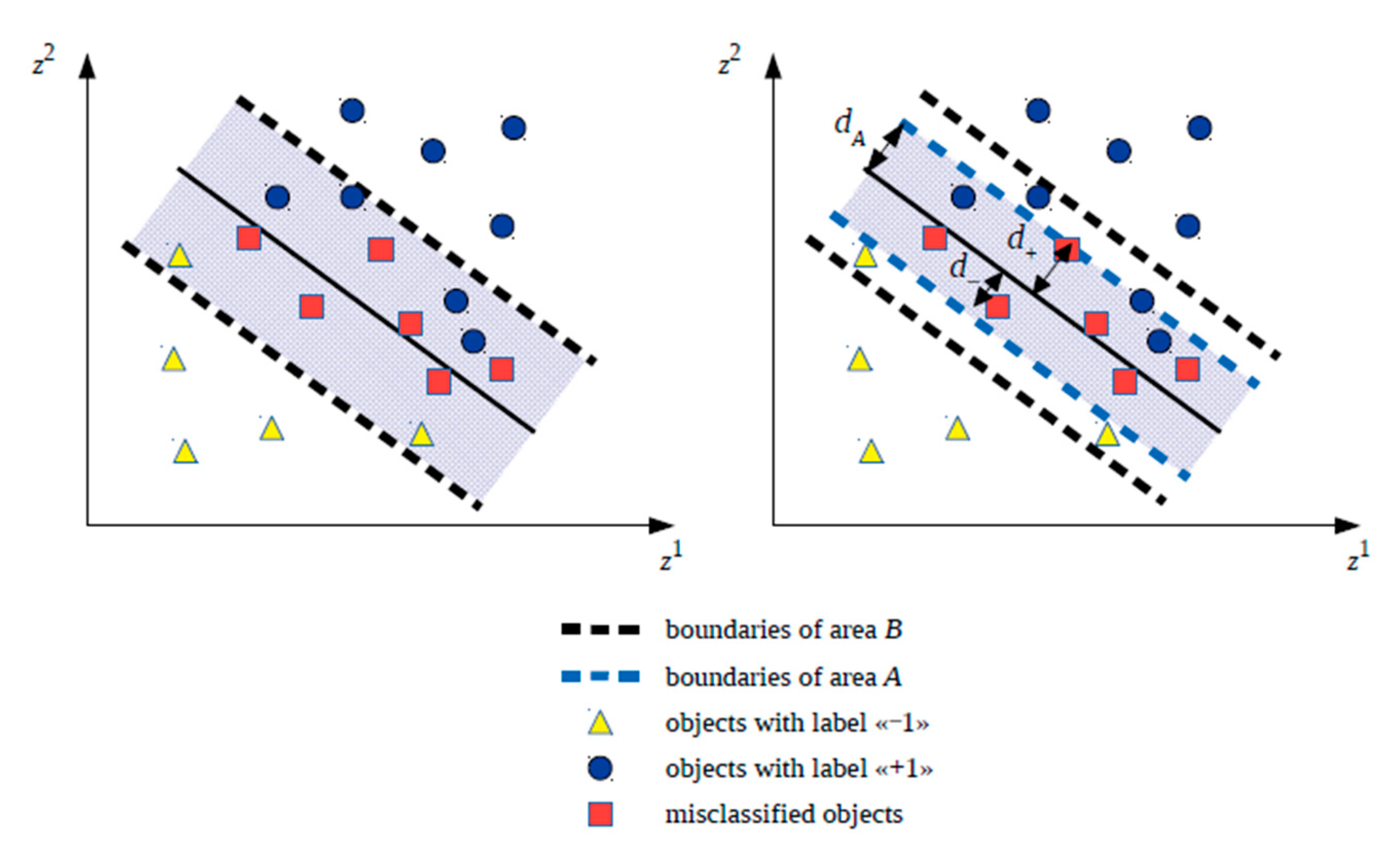
Variant 1. The training set for kNN classifier development includes all objects of the training set used at step 1.1 during SVM classifier development inside the strip separating the classes: $-1<w·z+b<1$. Let the area containing such objects be called $B$ (Boundary). In the future, symbol $B$ will be assigned to the corresponding hybrid classifier variant.

Variant 2. The training set for the kNN classifier development includes only those objects of the training set used at step 1.1 during training of the SVM classifier that fall into the area described by inequality $-{\rho }_A\le w·z+b\le {\rho }_A$, where ${\rho }_A$ is the number that satisfies inequality: $0<{\rho }_A<1$ and is defined as ${\rho }_A=\max ({\rho }_{-},{\rho }_{+})$, where ${\rho }_{-}$ is the maximum distance from the hyperplane separating the classes to the misclassified object of the class with the label “−1” belonging to the training set and located inside the strip separating classes; and ${\rho }_{+}$ is the maximum distance from the hyperplane separating the classes to the misclassified object of the class with the label “+1”, belonging to the training set and located inside the strip separating the classes. Let the area containing such objects be called $A$ (Area). In the future, symbol $A$ will be assigned to the corresponding hybrid classifier variant.

It should be noted that area $A$ with such a definition will be symmetric with respect to the hyperplane separating the classes, although it is possible to consider an asymmetric version for area $A$ in the future. While forming a training set for kNN classifier development based on objects from area $A$, it is assumed that in the future, thee SVM classifier will continue to correctly classify objects outside the area, and inside this area it will still sometimes make mistakes.

Let the area selected at step 1.2 be called $AorB$. It is assumed that the SVM classifier always makes mistakes within area $AorB$, otherwise kNN classifier development is not required. Figure A1 (Appendix A) shows examples of areas $A$ and $B$ in two-dimensional space.

Stage 2. kNN classifier development.

kNN classifier development is fulfilled on the basis on the training set formed at step 1.2 using one of two variants of the area $AorB$ (that is, area $A$ or $B$), for various values of the number k of nearest neighbors, various metrics for evaluating the distance between the objects (for example, in accordance with Formula (5)), and various voting rules (for example, in accordance with Formulas (6) or (7)). The best kNN classifier is selected so that it provides the highest quality of classification of all objects in the test set as a whole using the two-stage hybrid SVM-kNN classifier. Therefore, the parameter values of the best kNN classifier are fixed, in particular, the number of neighbors, metric for assessing the distance between objects, and voting rule are recorded.

The proposed two-stage hybrid SVM-kNN classifier implements cascade learning: first, on the basis of the training set, composed randomly from the considered dataset, the SVM classifier is trained, and then on the basis of the training set reduced in the above way, the kNN classifier is trained.

In the proposed two-stage hybrid SVM-kNN classifier, it is assumed that due to the development of the SVM classifier at the first stage, it is possible to change the balance of classes, working at the second stage in the development of the kNN classifier only with objects that fall into the reduced training dataset and inside the dividing strip (in area $A$ or $B$). Therefore, peripheral (uninformative) objects are excluded from the training dataset. These objects, in fact, do not affect the final decision (in particular, they are not support vectors and are not included in classification rules (2) or (4)).

It is reasonable to compare the results of the two-stage hybrid SVM-kNN classifier development with the results of the development of SVM and kNN classifiers that work with the default parameters values. As such, it will be possible to assess the expediency of using the two-stage hybrid SVM-kNN classifier to determine the class belonging of new objects, identifying or not identifying an increase in the values of the classification quality indicators of objects from the test set.

In the case of a positive decision on the expediency of using the developed two-stage hybrid SVM-kNN classifier, the classification of new objects can be performed as follows:

• apply the developed SVM classifier (with fixed parameters values) to separate new objects into two classes;
• select from the new objects those that fall into area $AorB$ built at step 1.2 at stage 1, and refine the classification decision for these objects using the developed kNN classifier.

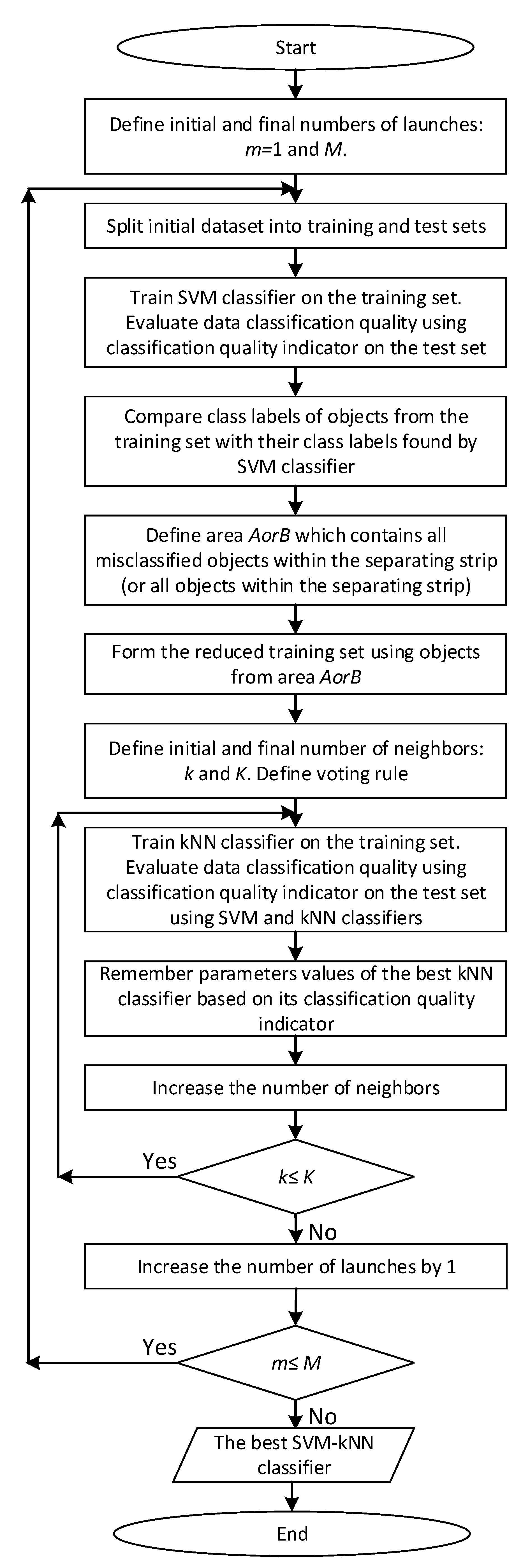
Figure 1 shows the enlarged block diagram of the two-stage hybrid SVM-kNN classifier development.

Two-stage hybrid SVM-kNN classifier development is implemented for various values of the number k of nearest neighbors. It is reasonable to use odd values of the number k when using votes majority rule (6) with the aim to avoid circumstances when the same number of neighbors voted for the various classes (in the case of binary classification).

During kNN classifier development, we worked with not only the entire training set, but with the reduced training set containing only the data about objects that fell into area $AorB$ (in the area $A$ or $B$), depending on which variant of the choice of the area turned out to be the best when developing the kNN classifier). The use of an auxiliary toolkit named as the kNN classifier, whose working principles are different from the working principles of SVM classifier, allows for an increase in the overall data classification quality in some cases.

The limitations on the applicability of the proposed two-stage hybrid SVM-kNN classifier are related to the fact that, due to the small width of area $AorB$ or excessive sparseness within area $AorB$, the size of the reduced training set (namely, the number of objects) may be insufficient for kNN classifier development.

5. Experimental Studies

The feasibility of using the proposed the two-stage hybrid versions of SVM-kNN classifiers was confirmed during experiments on real datasets taken from the UCI Machine Learning Repository and other sources applied to test the proposed classifiers.

The binary classification was implemented in all datasets that were used in experiments. Moreover, all datasets differed from each other by significantly different indicators of class imbalance. During the experiments, in particular, 20 datasets were considered (Australian, Banknote Authentication, Biodeg, Breast-Cancer-Wisconsin, Diabetic Retionopathy, German, Haberman, Heart, Ionosphere, Liver, Musk (Version 1), Musk (Version 2), Parkinsons, Phoneme, Pima Indians Diabetes, Spam, Sports Articles, Vertebral, LSVT Voice, WDBC), for three of which it was possible to obtain confirmation of the effectiveness of two-stage hybrid versions of SVM-kNN classifiers. The considered datasets are described in

Table A1. Datasets and their descriptions.

Dataset	Total Number of Objects s	Numberof Features q	Number of Objects in the Class with the Label “0”	Number of Objects in the Class with the Label “1”	Source
Australian	689	14	382	307	https://archive.ics.uci.edu/ml/datasets/statlog+(australian+credit+approval) (accessed on 10 December 2020)
Banknote Authentication	1371	4	761	610	https://archive.ics.uci.edu/ml/datasets/banknote+authentication (accessed on 10 December 2020)
Biodeg	1055	41	699	356	https://archive.ics.uci.edu/ml/datasets/SAR+biodegradation (accessed on 10 December 2020)
Breast-Cancer-Wisconsin	699	9	458	241	https://archive.ics.uci.edu/ml/datasets/breast+cancer+wisconsin+(diagnostic) (accessed on 10 December 2020)
Diabetic + Retinopathy	1150	19	84	41	https://archive.ics.uci.edu/ml/datasets/Diabetic+Retinopathy+Debrecen+Data+Set (accessed on 10 December 2020)
German	1000	24	700	300	http://archive.ics.uci.edu/ml/machine-learning-databases/statlog/german (accessed on 10 December 2020)
Haberman	305	3	224	81	https://archive.ics.uci.edu/ml/datasets/haberman%27s+survival (accessed on 10 December 2020)
Heart	270	13	150	120	http://archive.ics.uci.edu/ml/machine-learning-databases/statlog/heart (accessed on 10 December 2020)
Ionosphere	351	34	225	126	https://archive.ics.uci.edu/ml/machine-learning-databases/ionosphere (accessed on 10 December 2020)
Liver	345	6	200	145	http://archive.ics.uci.edu/ml/machine-learning-databases/liver-disorders (accessed on 10 December 2020)
LSVT Voice	125	310	84	41	http://archive.ics.uci.edu/ml/datasets/LSVT+Voice+Rehabilitation (accessed on 10 December 2020)
Musk (Version 1)	475	166	268	207	https://archive.ics.uci.edu/ml/datasets/Musk+(Version+1) (accessed on 10 December 2020)
Musk (Version 2)	6598	168	5580	1017	https://archive.ics.uci.edu/ml/datasets/Musk+(Version+2) (accessed on 10 December 2020)
Parkinsons	194	22	146	48	http://archive.ics.uci.edu/ml/datasets/Parkinsons (accessed on 10 December 2020)
Phoneme	5403	5	3817	1586	https://github.com/jbrownlee/Datasets/blob/master/phoneme.csv (accessed on 10 December 2020)
Pima Indians Diabetes	768	8	500	268	http://archive.ics.uci.edu/ml/datasets/Pima+Indians+Diabetes (accessed on 10 December 2020)
Spam	4601	57	2788	1813	https://archive.ics.uci.edu/ml/machine-learning-databases/spambase (accessed on 10 December 2020)
Sports Articles	1000	59	635	365	https://archive.ics.uci.edu/ml/datasets/Sports+articles+for+objectivity+analysis (accessed on 10 December 2020)
Vertebral	310	6	210	100	http://archive.ics.uci.edu/ml/datasets/Vertebral+Column (accessed on 10 December 2020)
WDBC	699	10	458	241	https://archive.ics.uci.edu/ml/datasets/Breast+Cancer+Wisconsin+(Diagnostic) (accessed on 10 December 2020)

(Appendix A). Objects of the majority class are marked with class label “0”, and objects of minority class are marked with class label “1” (for some datasets, class labels had to be renamed for consistency).

Software implementation was done in Python 3.8 using the Scikit-learn machine learning library, which provides tools for developing binary SVM, one-class SVM, and kNN classifiers. Jupyter Notebooks were applied to write the program code.

When developing SVM classifiers, implementations of binary and one-class SVM algorithms with default parameters values were used (

Table 1. Parameter values used by default in the SVM algorithms and kNN algorithm.

Name of Algorithm	Regulari-Zation Parameter C in the Binary SVM	$\mathit{n}\mathit{u}$ in the One-Class SVM	Type of Kernel Functionin Both SVMs	Value of Parameter of Kernel Function in Both SVMs	Distance Metric in kNN	Number of Neighbors in kNN	Weights for Neighbors in kNN	Algorithm Used to Compute the Nearest Neighbors in kNN	Leaf Size for Balltree or KDTree in kNN
Binary SVM	1	-	rbf	$1/(q·var(Z))$	-	-	-	-	-
One-class SVM		0.5	rbf	$1/(q·var(Z))$	-	-	-	-	-
kNN	-	-	-	-	euclidean	5	uniform	auto	30

). When developing the kNN classifiers, implementation of the kNN algorithm with the default parameter values (Table 1) was used as well as the implementation of the kNN algorithm in which the number of neighbors was chosen from the range [5,46] with the step equal to 2 (with voting by a majority of votes and weighted voting).

Table 1 uses the following notations:

• $nu$ is the lower boundary of the portion of support vectors and the upper boundary on the portion of training errors ($nu\in (0,1]$);
• $var(Z)$ is the training dataset variance calculated as: $var(Z)=mean({(Z-mean(Z))}^2)$; $mean(Z)=sum(Z)/S$;
• $S$ is the number of objects in the training set;
• $q$ is the number of features;
• rbf is the radial basis kernel function; and
• auto means that the most appropriate algorithm from BallTree, KDTree, Brute-force search is used.

The portion of the test set was equal to 20% of the considered dataset.

During the experiments, the following versions of the classifiers were developed.

• kNN classifier with default parameter values, named as kNN-default.
• kNN classifier, which implements the search for the best number of neighbors with the rest default parameter values, named as kNN.
• Binary SVM classifier with default parameter values, named as bSVM-default.
• One-class SVM-classifier, working in the role of a binary, with default parameter values, named as obSVM-default.
• A hybrid of the binary SVM classifier with default parameter values and kNN classifier, which implements the search for the best number of neighbors with the rest default parameter values, and takes into account the boundaries of the strip separating the classes, named as bSVM-B-kNN.
• A hybrid of the one-class SVM classifier, working as a binary, with default parameter values, and kNN classifier, which implements the search for the best number of neighbors with the rest default parameter values, and takes into account the boundaries of the strip separating the classes, named as obSVM-B-kNN.
• A hybrid of a binary SVM classifier with default parameter values and a kNN classifier that realizes the search for the best number of neighbors with the default parameter values, and takes into account the selected symmetric areas within the boundaries defining the band separating the classes, named as bSVM-A-kNN.
• A hybrid of a one-class SVM classifier, working as a binary, with the default parameter values, and a kNN classifier, which realizes the search for the best number of neighbors with the rest default parameter values, and takes into account the selected symmetric area within the boundaries, defining the strip separating the classes, named as obSVM-A-kNN.

Before the training procedure, the values of the elements of the feature vectors of objects were scaled: standardization (Standard) and MinMax scaling techniques were used in order to select the best one based on the results of training. In the overwhelming majority of cases, the best learning outcomes (in terms of the classification quality) were obtained using standardization.

The quality of the classifiers was assessed on the test set using classification quality indicators such as Balanced Accuracy (BA), Accuracy (Acc), and $F_1$-score ($F_1$). For each fixed number of neighbors, 500 random partitions of the dataset were performed into test and training sets in a ratio of 80:20, followed by training, testing, and choosing the best hybrid classifier (including choosing the best number of neighbors in the kNN classifier) to sense this or that indicator of the quality of the classification.

The calculation of indicators $BA$, $Acc$, and $F_1$ in the case of binary classification was carried out in accordance with formulas:

$$BA=\frac{1}{2}·\left(Sensitivity+Specificity\right)=\frac{1}{2}·\left(\frac{TP}{TP+FN}+\frac{TN}{TN+FP}\right),$$

(8)

$$Acc=\frac{TP+TN}{TP+FN+TN+FP},$$

(9)

$$F_1=2·\frac{Precision·Recall}{Precision+Recall}=\frac{2·TP}{2·TP+FN+FP},$$

(10)

where $TP$ is the number of true positive outcomes; $TN$ is the number of true negative outcomes; $FP$ is the number of false positive outcomes; $FN$ is the number of false negative outcomes; $Sensitivity =Recall=\frac{TP}{TP+FN}$; $Specificity =\frac{TN}{TN+FP}$; and $Precision=\frac{TP}{TP+FP}$.

The balanced accuracy indicator $BA$ differs from the accuracy indicator $Acc$ in that the proportion of objects in each of the classes is taken into account when calculating it. Hence, indicator $BA$ gives the most reliable assessment of the classification quality of unbalanced datasets.

5.1. Hybrid Classifier Development Using kNN Classifier Based on the Votes Majority Rule

First, the experiments for the case when the votes majority rule according to Formula (6) is used in the development of the kNN classifier were carried out.

During the experiments, it was possible to prove the effectiveness of the proposed two-stage hybrid classifiers using three datasets such as Haberman, Heart, and Pima Indians Diabetes. The efficiency of the proposed two-stage hybrid classifiers for four more datasets such as Breast-Cancer-Wisconsin, Parkinsons, LSVT Voice, and WDBC turned out to be the same as when using the kNN classifier, for which the search for the optimal number of neighbors was carried out.

Table 2. Values of balanced accuracy indicator (when votes majority rule (6) is used in the kNN classifier).

Dataset/Scaling Method	kNN/Number of Neighbors	kNN-default	SVM-default	obSVM-default	bSVM-A-kNN/Number of Neighbors	bSVM-B-kNN/Number of Neighbors	obSVM-A-kNN/Number of Neighbors	obSVM-B-kNN/Number of Neighbors
Haberman/Standard	0.829/25	0.763	0.775	0.784	0.780/17	0.771/17	0.839/23	0.829/33
Haberman/MinMax	0.776/13	0.761	0.731	0.784	0.798/15	0.798/15	0.745/11	0.789/11
Heart/Standard	0.984/35	0.963	0.963	0.766	0.832/25	0.867/23	0.907/35	0.955/43
Heart/MinMax	0.982/29	0.96	0.972	0.762	0.809/31	0.816/35	0.905/5	0.903/25
Pima Indians Diabetes/Standard	0.810/7	0.805	0.828	0.722	0.711/41	0.730/35	0.795/41	0.813/17
Pima Indians Diabetes/MinMax	0.814/21	0.801	0.839	0.738	0.718/5	0.732/7	0.777/33	0.786/13

,

Table 3. Values of accuracy indicator (when votes majority rule (6) is used in the kNN classifier).

Dataset/Scaling Method	kNN/Number of Neighbors	kNN-default	SVM-default	obSVM-default	bSVM-A-kNN/Number of Neighbors	bSVM-B-kNN/Number of Neighbors	obSVM-A-kNN/Number of Neighbors	obSVM-B-kNN/Number of Neighbors
Haberman/Standard	0.918/21	0.869	0.918	0.754	0.918/23	0.918/23	0.934/23	0.918/17
Haberman/MinMax	0.902/13	0.869	0.902	0.738	0.905/37	0.905/39	0.902/37	0.902/23
Heart/Standard	0.981/11	0.963	0.963	0.759	0.852/25	0.870/17	0.926/31	0.963/27
Heart/MinMax	0.981/29	0.963	0.963	0.759	0.815/13	0.833/19	0.907/5	0.907/15
Pima Indians Diabetes/Standard	0.864/17	0.831	0.857	0.708	0.799/19	0.818/41	0.864/41	0.870/17
Pima Indians Diabetes/MinMax	0.857/21	0.851	0.864	0.721	0.799/17	0.792/5	0.844/19	0.851/33

and

Table 4. Values of $F_1$-score indicator (when votes majority rule (6) is used in the kNN classifier).

Dataset/Scaling Method	kNN/Number of Neighbors	kNN-default	SVM-default	obSVM-default	bSVM-A-kNN/Number of Neighbors	bSVM-B-kNN/Number of Neighbors	obSVM-A-kNN/Number of Neighbors	obSVM-B-kNN/Number of Neighbors
Haberman/Standard	0.700/33	0.636	0.666	0.667	0.700/11	0.700/11	0.727/11	0.667/23
Haberman/MinMax	0.667/13	0.600	0.588	0.642	0.700/15	0.700/15	0.640/11	0.667/11
Heart/Standard	0.980/11	0.963	0.962	0.780	0.800/25	0.851/23	0.895/31	0.952/43
Heart/MinMax	0.982/29	0.958	0.962	0.788	0.773/31	0.792/17	0.894/7	0.894/25
Pima Indians Diabetes/Standard	0.755/7	0.752	0.763	0.680	0.605/25	0.636/25	0.727/41	0.738/17
Pima Indians Diabetes/MinMax	0.750/23	0.742	0.804	0.667	0.612/5	0.653/7	0.702/11	0.719/13

show the classification quality indicator values (Balanced Accuracy (BA), Accuracy (Acc), $F_1$-score ($F_1$)) and the number of neighbors for which the best (i.e., maximum) classification quality indicator value was reached, for three datasets (Haberman, Heart, Pima Indians Diabetes), on which the successful application of two-stage hybrid versions of SVM-kNN classifiers (when at least one of the three indicators is clearly improved or the obtained decision is among the top three out of eight classifiers above-mentioned) is observed. The class was assigned to the object $z$ in accordance with the votes majority rule (6).

In Table 2, Table 3 and Table 4, indicator values that occupy the first place are highlighted in bold, indicator values that occupy second place are highlighted in bold italics, and indicator values that occupy the third place are simply italicized (when ranking in descending order of indicators values).

As can be seen from Table 2, Table 3 and Table 4, all four versions of the two-stage hybrid SVM-kNN classifiers (bSVM-A-kNN, bSVM-B-kNN, obSVM-A-kNN, obSVM-B-kNN) took the lead on different datasets (or are included in the top three) when analyzing certain classification quality indicators, in connection with which it is possible to talk about their effectiveness and expediency of use (especially in the case of further fine tuning of SVM classifier parameter values).

For another four datasets (Breast-Cancer-Wisconsin, Parkinsons, LSVT Voice, and WDBC), it turned out that the kNN, kNN-default, SVM-default classifiers and two-stage hybrid SVM-kNN classifiers provided the same values of the classification quality indicators ($BA$, $Acc$, $F_1$) equal to 1 on the test set. Therefore, the class was assigned to object $z$ in accordance with the votes majority rule (6). The main difference between two-stage hybrid SVM-kNN classifiers and kNN classifiers is, possibly, in a various number of neighbors, at which the best (i.e., maximum) value of the classification quality indicator was reached. Thus, the composition of the training and test sets, with the use of which the best (i.e., maximum) value of the classification quality indicator was achieved, can be obtained in different ways (with various composition of training and test sets and various numbers of neighbors in kNN classifier), while, generally speaking, the time to obtain the desired high-quality classifier can be minimized by developing the kNN classifier, which is part of the two-stage hybrid SVM-kNN classifier, due to the use of the training set of lower cardinality than in the case when only kNN or SVM classifiers are developed.

Table 5. Number of neighbors at which the maximum classification quality indicators values were achieved on the Breast-Cancer-Wisconsin dataset (when votes majority rule (6) is used in the kNN classifier).

Classification Quality Indicator	kNN: Standard/MinMax	bSVM-A-kNN: Standard/MinMax	bSVM-B-kNN: Standard/MinMax	obSVM-A-kNN: Standard/MinMax	obSVM-B-kNN: Standard/MinMax
$BA$	5/5	-	-	7/5	5/5
$Acc$	5/5	-	-	7/5	5/5
$F_1$	5/5	-	-	7/5	5/5

,

Table 6. Number of neighbors at which the maximum classification quality indicators values were achieved on the Parkinsons dataset (when votes majority rule (6) is used in the kNN classifier).

Classification Quality Indicator	kNN: Standard/MinMax	bSVM-A-kNN: Standard/MinMax	bSVM-B-kNN: Standard/MinMax	obSVM-A-kNN: Standard/MinMax	obSVM-B-kNN: Standard/MinMax
$BA$	5/5	-	9/-	5/5	9/9
$Acc$	5/5	-	9/-	5/5	9/9
$F_1$	5/5	-	9/-	5/5	9/9

,

Table 7. Number of neighbors at which the maximum classification quality indicators values were achieved on the LSVT Voice dataset (when votes majority rule (6) is used in the kNN classifier).

Classification Quality Indicator	kNN: Standard/MinMax	bSVM-A-kNN: Standard/MinMax	bSVM-B-kNN: Standard/MinMax	obSVM-A-kNN: Standard/MinMax	obSVM-B-kNN: Standard/MinMax
$BA$	5/5	17/5	9/5	-	-
$Acc$	5/5	17/5	9/5	-	-
$F_1$	5/5	17/5	9/5	-	-

and

Table 8. Number of neighbors at which the maximum classification quality indicators values were achieved on the WDBC dataset (when votes majority rule (6) is used in the kNN classifier).

Classification Quality Indicator	kNN: Standard/MinMax	bSVM-A-kNN: Standard/MinMax	bSVM-B-kNN: Standard/MinMax	obSVM-A-kNN: Standard/MinMax	obSVM-B-kNN: Standard/MinMax
$BA$	5/5	-	-	5/5	5/5
$Acc$	5/5	-	-	5/5	5/5
$F_1$	5/5	-	-	5/5	5/5

show the number of neighbors for the Standard and MinMax scaling methods, at which the best (i.e., maximum) values of classification quality indicators were achieved in the kNN, bSVM-A-kNN, bSVM-B-kNN, obSVM-A-kNN, and obSVM-B-kNN classifiers for different classification quality indicators on the Breast-Cancer-Wisconsin, Parkinsons, LSVT Voice, and WDBC datasets. Dashes (“-”) in the cells of Table 5, Table 6, Table 7 and Table 8 mean that for the classifier named in the column heading, the maximum value of the quality indicator named in the row headings (in the leftmost cell of the row) was not observed.

Appendix B provides

Table A2. Values of the balanced accuracy indicator (when votes majority rule (6) is used in the kNN classifier).

Dataset/Scaling Method	kNN/Number of Neighbors	kNN-default	SVM-default	obSVM-default	bSVM-A-kNN/Number of Neighbors	bSVM-B-kNN/Number of Neighbors	obSVM-A-kNN/Number of Neighbors	obSVM-B-kNN/Number of Neighbors
Australian/Standard	0.942/27	0.935	0.941	0.689	0.721/5	0.749/5	0.841/23	0.848/41
Australian/MinMax	0.945/45	0.931	0.950	0.647	0.687/15	0.730/15	0.831/45	0.837/35
German/Standard	0.754/5	0.754	0.763	0.684	0.705/5	0.706/5	0.674/7	0.669/5
German/MinMax	0.730/5	0.730	0.755	0.659	0.693/7	0.693/9	0.673/7	0.673/7
Ionosphere/Standard	0.944/5	0.944	1	0.937	0.656/19	0.792/5	0.889/5	0.900/19
Ionosphere/MinMax	0.944/5	0.944/5	1	0.895	0.678/11	0.727/5	0.875/17	0.881/17

,

Table A3. Values of the accuracy indicator (when votes majority rule (6) is used in the kNN classifier).

Dataset/Scaling Method	kNN/Number of Neighbors	kNN-default	SVM-default	obSVM-default	bSVM-A-kNN/Number of Neighbors	bSVM-B-kNN/Number of Neighbors	obSVM-A-kNN/Number of Neighbors	obSVM-B-kNN/Number of Neighbors
Australian/Standard	0.949/27	0.935	0.942	0.689	0.721/5	0.749/5	0.877/23	0.848/41
Australian/MinMax	0.945/45	0.931	0.950	0.647	0.687/15	0.730/15	0.831/45	0.837/35
German/Standard	0.825/27	0.815/5	0.850	0.655	0.825/41	0.825/27	0.825/41	0.825/41
German/MinMax	0.820/19	0.820	0.865	0.640	0.823/19	0.822/19	0.825/23	0.810/15
Ionosphere/Standard	0.972/5	0.972	1	0.930	0.803/13	0.859/5	0.930/5	0.944/19
Ionosphere/MinMax	0.972/5	0.972	1	0.887	0.859/19	0.859/11	0.930/11	0.930/7

and

Table A4. Values of the $F_1$-score indicator (when votes majority rule (6) is used in the kNN classifier).

Dataset/Scaling Method	kNN/Number of Neighbors	kNN-default	SVM-default	obSVM-default	bSVM-A-kNN/Number of Neighbors	bSVM-B-kNN/Number of Neighbors	obSVM-A-kNN/Number of Neighbors	obSVM-B-kNN/Number of Neighbors
Australian/Standard	0.937/27	0.933	0.934	0.694	0.628/5	0.674/5	0.817/31	0.824/41
Australian/MinMax	0.940/9	0.925	0.945	0.667	0.578/15	0.653/15	0.800/45	0.814/35
German/Standard	0.593/5	0.620/5	0.680	0.592	0.595/5	0.595/5	0.523/7	0.521/5
German/MinMax	0.590/5	0.618	0.667	0.556	0.564/7	0.566/9	0.526/7	0.526/7
Ionosphere/Standard	0.941/5	0.941	1	0.902	0.485/9	0.737/5	0.875/5	0.889/19
Ionosphere/MinMax	0.941/5	0.941	1	0.868	0.522/11	0.625/5	0.857/17	0.865/17

, which show the classification quality indicator values (and number of neighbors) for which the best (i.e., maximum) classification quality indicator value was reached for three datasets (Australian, German, and Ionosphere) on which the successful application of two-stage hybrid versions of SVM-kNN classifiers was not obtained. Therefore, the class was assigned to the object $z$ in accordance with the votes majority rule (6).

The success of applying the proposed two-stage hybrid versions of SVM-kNN classifiers to some datasets and the failure of their application to others can be explained by the peculiarities of forming area $AorB$ or grouping objects of the training set within area $AorB$.

5.2. Hybrid Classifier Development Using kNN Classifier Based on the Rule of Weighted Voting

Similar experiments for the case when the rule of weighted voting according to Equation (7) used in the development of the kNN classifier were carried out.

During the experiments, it was possible to prove the effectiveness of the proposed two-stage hybrid classifiers using three datasets such as Haberman, Heart, and Pima Indians Diabetes. The efficiency of the proposed two-stage hybrid classifiers for four more datasets such as Breast-Cancer-Wisconsin, Parkinsons, LSVT Voice, and WDBC turned out to be the same as when using the kNN classifier, for which the search for the optimal number of neighbors was carried out.

Table 9. Values of balanced accuracy indicator (when rule of weighted voting (7) is used in the kNN classifier).

Dataset/Scaling Method	kNN/Number of Neighbors	kNN-default	SVM-default	obSVM-default	bSVM-A-kNN/Number of Neighbors	bSVM-B-kNN/Number of Neighbors	obSVM-A-kNN/Number of Neighbors	obSVM-B-kNN/Number of Neighbors
Haberman/Standard	0.918/21	0.869	0.918	0.754	0.918/23	0.918/23	0.934/23	0.918/17
Haberman/MinMax	0.902/13	0.869	0.902	0.738	0.905/37	0.905/39	0.902/37	0.902/23
Heart/Standard	0.981/11	0.963	0.963	0.759	0.852/25	0.870/17	0.926/31	0.963/27
Heart/MinMax	0.981/29	0.963	0.963	0.759	0.815/13	0.833/19	0.907/5	0.907/15
Pima Indians Diabetes/Standard	0.864/17	0.831	0.857	0.708	0.799/19	0.818/41	0.864/41	0.870/17
Pima Indians Diabetes/MinMax	0.857/21	0.851	0.864	0.721	0.799/17	0.792/5	0.844/19	0.851/33

,

Table 10. Values of accuracy indicator (when rule of weighted voting (7) is used in the kNN classifier).

Dataset/Scaling Method	kNN/Number of Neighbors	kNN-default	SVM-default	obSVM-default	bSVM-A-kNN/Number of Neighbors	bSVM-B-kNN/Number of Neighbors	obSVM-A-kNN/Number of Neighbors	obSVM-B-kNN/Number of Neighbors
Haberman/Standard	0.918/23	0.869	0.918	0.754	0.934/29	0.918/23	0.918/23	0.918/45
Haberman/MinMax	0.902/25	0.869	0.902	0.738	0.902/23	0.902/25	0.902/25	0.885/19
Heart/Standard	0.981/43	0.963	0.963	0.759	0.870/27	0.887/19	0.963/43	0.963/15
Heart/MinMax	0.981/39	0.963	0.963	0.759	0.852/5	0.870/25	0.907/7	0.926/21
Pima Indians Diabetes/Standard	0.870/11	0.831	0.857	0.708	0.805/17	0.825/29	0.851/41	0.857/41
Pima Indians Diabetes/MinMax	0.864/19	0.851	0.864	0.721	0.799/15	0.799/15	0.851/23	0.857/43

and

Table 11. Values of $F_1$-score indicator (when rule of weighted voting (7) is used in the kNN classifier).

Dataset/Scaling Method	kNN/Number of Neighbors	kNN-default	SVM-default	obSVM-default	bSVM-A-kNN/Number of Neighbors	bSVM-B-kNN/Number of Neighbors	obSVM-A-kNN/Number of Neighbors	obSVM-B-kNN/Number of Neighbors
Haberman/Standard	0.737/29	0.636	0.666	0.667	0.778/29	0.737/29	0.696/17	0.640/7
Haberman/MinMax	0.667/19	0.600	0.588	0.642	0.667/13	0.667/13	0.609/13	0.571/9
Heart/Standard	0.979/13	0.963	0.962	0.780	0.800/33	0.840/19	0.952/43	0.952/45
Heart/MinMax	0.978/39	0.958	0.962	0.788	0.778/5	0.780/37	0.894/43	0.894/7
Pima Indians Diabetes/Standard	0.783/11	0.752	0.763	0.680	0.625/29	0.651/37	0.721/35	0.721/43
Pima Indians Diabetes/MinMax	0.774/19	0.742	0.804	0.667	0.629/11	0.653/5	0.698/27	0.711/43

show the classification quality indicator values (BA, Acc, $F_1$) and number of neighbors for which the best (i.e., maximum) classification quality indicator value was reached for three datasets (Haberman, Pima Indians Diabetes, Heart), on which the successful application of two-stage hybrid versions of SVM-kNN classifiers (when at least one of the three indicators is clearly improved or the obtained decision is in the top three out of eight classifiers above-mentioned) is observed. Therefore, the class was assigned to the object $z$ in accordance with the rule of weighted voting (7).

In Table 9, Table 10 and Table 11, the indicator values that occupy the first place are highlighted in bold; indicator values that occupy the second place are highlighted in bold italics; and indicator values that occupy the third place are simply italicized (when ranking in descending order of indicators values).

As can be seen from Table 9, Table 10 and Table 11, all four versions of the two-stage hybrid SVM-kNN classifiers (bSVM-A-kNN, bSVM-B-kNN, obSVM-A-kNN, obSVM-B-kNN) took the lead on different datasets (or are included in the top three) when analyzing certain classification quality indicators, in connection with which it is possible to talk about their effectiveness and expediency of use (especially in the case of more fine tuning of the values of SVM classifier parameters).

For another four datasets (Breast-Cancer-Wisconsin, Parkinsons, LSVT Voice, and WDBC), it turned out that the kNN, kNN-default, SVM-default classifiers, and two-stage hybrid SVM-kNN classifiers gave the same values of the classification quality indicators ($BA$, $Acc$, $F_1$), equal to 1 on the test set. The class was assigned to object $z$ in accordance with the rule of weighted voting (7). The main difference between the two-stage hybrid SVM-kNN classifiers and kNN classifiers (the same as when using the votes majority rule (6)) is, possibly, in a various number of neighbors at which the best (i.e., maximum) value of the classification quality indicator was achieved. The composition of the training and test sets, with the use of which the best (i.e., maximum) value of the classification quality indicator was achieved, can be obtained in different ways (with various compositions of training and test sets and various numbers of neighbors in the kNN classifier), while, generally speaking, the time required to obtain the desired high-quality classifier can be minimized by developing the kNN classifier, which is part of the two-stage hybrid SVM-kNN classifier, due to the use of the training set of lower cardinality than in the case when only kNN or SVM classifiers are developed.

Table 12. Number of neighbors at which the maximum values of classification quality indicators were achieved on the Breast-Cancer-Wisconsin dataset (when rule of weighted voting (7) is used in the kNN classifier).

Classification Quality Indicator	kNN: Standard/MinMax	bSVM-A-kNN: Standard/MinMax	bSVM-B-kNN: Standard/MinMax	obSVM-A-kNN: Standard/MinMax	obSVM-B-kNN: Standard/MinMax
$BA$	5/5	-	-	5/5	5/5
$Acc$	5/5	-	-	5/5	5/5
$F_1$	5/5	-	-	5/5	5/5

,

Table 13. Number of neighbors at which the maximum values of classification quality indicators were achieved on the Parkinsons dataset (when rule of weighted voting (7) is used in the kNN classifier).

Classification Quality Indicator	kNN: Standard/MinMax	bSVM-A-kNN: Standard/MinMax	bSVM-B-kNN: Standard/MinMax	obSVM-A-kNN: Standard/MinMax	obSVM-B-kNN: Standard/MinMax
$BA$	5/5	21/9	9/9	7/5	5/5
$Acc$	5/5	21/9	9/9	7/5	5/5
$F_1$	5/5	21/9	9/9	7/5	5/5

,

Table 14. Number of neighbors at which the maximum values of classification quality indicators were achieved on the LSVT Voice dataset (when rule of weighted voting (7) is used in kNN classifier).

Classification Quality Indicator	kNN: Standard/MinMax	bSVM-A-kNN: Standard/MinMax	bSVM-B-kNN: Standard/MinMax	obSVM-A-kNN: Standard/MinMax	obSVM-B-kNN: Standard/MinMax
$BA$	5/5	21/-	9/9	-	-/11
$Acc$	5/5	21/-	9/9	-	-/11
$F_1$	5/5	21/-	9/9	-	-/11

and

Table 15. Number of neighbors at which the maximum values of classification quality indicators were achieved on the WDBC dataset (when rule of weighted voting (7) is used in the kNN classifier).

Classification Quality Indicator	kNN: Standard/MinMax	bSVM-A-kNN: Standard/MinMax	bSVM-B-kNN: Standard/MinMax	obSVM-A-kNN: Standard/MinMax	obSVM-B-kNN: Standard/MinMax
$BA$	5/5	-	-	7/5	7/5
$Acc$	5/5	-	-	7/5	7/5
$F_1$	5/5	-	-	7/5	7/5

show the number of neighbors for the Standard and MinMax scaling methods, at which the best (i.e., maximum) values of classification quality indicators were achieved in the kNN, bSVM-A-kNN, bSVM-B-kNN, obSVM-A-kNN, obSVM-B-kNN classifiers for different classification quality indicators on the Breast-Cancer-Wisconsin, Parkinsons, LSVT Voice, and WDBC datasets. Dashes (“-”) in the cells of Table 12, Table 13, Table 14 and Table 15 mean that for the classifier named in the column heading, the maximum value of the quality indicator named in the row headings (in the leftmost cell of the row) was not observed.

It should be noted that one of the kNN classifiers, named in Table 2, Table 3, Table 4, Table 5, Table 6, Table 7, Table 8, Table 9, Table 10, Table 11, Table 12, Table 13, Table 14 and Table 15 as kNN, implements the search for the best number of neighbors. However, this does not always allow this classifier to become the winner among the considered classifiers in terms of $BA$, $Acc$, and $F_1$. kNN-default, SVM-default, obSVM-default classifiers work with the default parameters values.

Appendix B provides

Table A5. Values of the balanced accuracy indicator (when rule of weighted voting (7) is used in the kNN classifier).

Dataset/Scaling Method	kNN/Number of Neighbors	kNN-default	SVM-default	obSVM-default	bSVM-A-kNN/Number of Neighbors	bSVM-B-kNN/Number of Neighbors	obSVM-A-kNN/Number of Neighbors	obSVM-B-kNN/Number of Neighbors
Australian/Standard	0.940/23	0.935	0.941	0.689	0.708/23	0.738/41	0.850/15	0.835/25
Australian/MinMax	0.945/23	0.935	0.950	0.647	0.687/39	0.730/39	0.826/43	0.833/23
German/Standard	0.754/5	0.754	0.763	0.684	0.687/5	0.685/17	0.661/15	0.672/9
German/MinMax	0.742/5	0.729	0.753	0.668	0.692/13	0.700/13	0.692/9	0.682/21
Ionosphere/Standard	0.944/5	0.944	1	0.937	0.694/17	0.740/15	0.875/15	0.900/11
Ionosphere/MinMax	0.944/5	0.944	1	0.895	0.676/5	0.740/21	0.880/5	0.881/17

,

Table A6. Values of the accuracy indicator (when rule of weighted voting (7) is used in the kNN classifier).

Dataset/Scaling Method	kNN/Number of Neighbors	kNN-default	SVM-default	obSVM-default	bSVM-A-kNN/Number of Neighbors	BSVM-B-kNN/Number of Neighbors	obSVM-A-kNN/Number of Neighbors	obSVM-B-kNN/Number of Neighbors
Australian/Standard	0.940/23	0.935	0.942	0.689	0.783/33	0.783/33	0.870/13	0.835/25
Australian/MinMax	0.945/23	0.935	0.950	0.647	0.687/39	0.730/39	0.826/43	0.833/23
German/Standard	0.840/39	0.810	0.850	0.655	0.820/17	0.835/17	0.820/17	0.825/25
German/MinMax	0.840/13	0.820	0.865	0.640	0.825/13	0.825/13	0.825/13	0.815/5
Ionosphere/Standard	0.972/5	0.972	1	0.930	0.845/17	0.859/9	0.930/7	0.944/11
Ionosphere/MinMax	0.972/5	0.972	1	0.887	0.845/5	0.859/11	0.930/7	0.930/13

and

Table A7. Values of the $F_1$-score indicator (when rule of weighted voting (7) is used in the kNN classifier).

Dataset/Scaling Method	kNN/Number of Neighbors	kNN-default	SVM-default	obSVM-default	bSVM-A-kNN/Number of Neighbors	bSVM-B-kNN/Number of Neighbors	obSVM-A-kNN/Number of Neighbors	obSVM-B-kNN/Number of Neighbors
Australian/Standard	0.934/23	0.933/5	0.934	0.694	0.607/5	0.660/41	0.824/15	0.810/19
Australian/MinMax	0.940/17	0.932	0.945	0.667	0.578/39	0.653/39	0.793/37	0.804/23
German/Standard	0.620/5	0.620	0.680	0.592	0.544/11	0.544/11	0.495/9	0.518/9
German/MinMax	0.635/9	0.618	0.667	0.556	0.565/5	0.565/5	0.559/9	0.532/21
Ionosphere/Standard	0.980/5	0.980	1	0.902	0.560/17	0.649/15	0.857/15	0.889/11
Ionosphere/MinMax	0.942/5	0.942	1	0.868	0.526/9	0.649/21	0.864/5	0.865/17

, which show the classification quality indicator values (and number of neighbors for which the best (i.e., maximum) classification quality indicator value was reached, for three datasets (Australian, German, and Ionosphere) on which successful application of two-stage hybrid versions of SVM-kNN classifiers was not obtained. Thus, the class was assigned to the object $z$ in accordance with the rule of weighted voting (7).

It should be additionally noted, according to the results of the data analysis in Table 2, Table 3, Table 4, Table 5, Table 6, Table 7, Table 8, Table 9, Table 10, Table 11, Table 12, Table 13, Table 14 and Table 15, that in some cases, the use of the rule of weighted voting (7) in kNN classifier development can improve the classification quality.

5.3. Analysis of Class Imbalance in Initial and Reduced Training Sets

Table 16. Statistics for the number and ratio of objects of different classes in training sets with the best values of the balanced accuracy indicator.

Dataset	Name of Classifier	Success of Hybrid Application (Whether It Took 1st Place among 7 Classifiers, with the Exclusion of kNN from the List of 8 Classifiers)	Ratio of Number of Objects Labeled “0” and “1” in the Initial Training Set	Ratio of Number of Objects Labeled “0” and “1” in the AorB Area Separating the Classes in SVM Classifier
Australian	obSVM-A-kNN	−	295/256 = 1.152	271/224 = 1.210
	bSVM-A-kNN	−	299/252 = 1.187	272/220 = 1.236
	obSVM-B-kNN	−	313/238 = 1.315	288/215 = 1.340
	bSVM-B-kNN	−	306/245 = 1.249	279/220 = 1.268
Breast-Cancer-Wisconsin	obSVM-A-kNN	+	363/196 = 1.852	294/191 = 1.539
	bSVM-A-kNN	−	369/190 = 1.942	298/188 = 1.585
	obSVM-B-kNN	+	363/196 = 1.852	303/192 = 1.578
	bSVM-B-kNN	−	365/194 = 1.881	280/193 = 1.451
German	obSVM-A-kNN	−	558/242 = 2.306	509/226 = 2.252
	bSVM-A-kNN	−	568/232 = 2.448	528/219 = 2.411
	obSVM-B-kNN	−	560/240 = 2.333	513/220 = 2.332
	bSVM-B-kNN	−	557/243 = 2.292	513/223 = 2.300
Haberman	obSVM-A-kNN	+	170/74 = 2.297	140/65 = 2.154
	bSVM-A-kNN	−	173/71 = 2.437	144/62 = 2.323
	obSVM-B-kNN	−	170/74 = 2.297	140/65 = 2.154
	bSVM-B-kNN	−	172/72 = 2.389	133/66 = 2.015
Heart	obSVM-A-kNN	−	115/101 = 1.139	77/74 = 1.041
	bSVM-A-kNN	−	118/98 = 1.204	86/73 = 1.178
	obSVM-B-kNN	−	118/98 = 1.204	80/75 = 1.067
	bSVM-B-kNN	−	122/94 = 1.298	90/70 = 1.286
Ionosphere	obSVM-A-kNN	−	181/99 = 1.828	158/93 = 1.699
	bSVM-A-kNN	−	186/94 = 1.979	166/86 = 1.930
	obSVM-B-kNN	−	174/106 = 1.642	155/99 = 1.566
	bSVM-B-kNN	−	175/105 = 1.667	157/99 = 1.586
LSVT Voice	obSVM-A-kNN	−	65/35 = 1.857	39/24 = 1.625
	bSVM-A-kNN	+	69/31 = 2.256	45/21 = 2.143
	obSVM-B-kNN	−	65/35 = 1.857	41/22 = 1.864
	bSVM-B-kNN	+	68/32 = 2.125	41/21 = 1.952
Parkinsons	obSVM-A-kNN	+	111/44 = 2.523	77/33 = 2.333
	bSVM-A-kNN	−	110/45 = 2.444	83/30 = 2.767
	obSVM-B-kNN	+	111/44 = 2.523	83/30 = 2.767
	bSVM-B-kNN	+	111/44 = 2.523	82/31 = 2.645
Pima Indians Diabetes	obSVM-A-kNN	−	390.224 = 1.741	360/213 = 1.690
	bSVM-A-kNN	−	395/219 = 1.804	367/208 = 1.764
	obSVM-B-kNN	+	383/231 = 1.658	356/217 = 1.641
	bSVM-B-kNN	−	401/213 = 1.883	369/202 = 1.827
WDBC	obSVM-A-kNN	+	374/185 = 2.022	316/181 = 1.746
	bSVM-A-kNN	−	366/192 = 1.896	302/192 = 1.573
	obSVM-B-kNN	+	365/194 = 1.881	306/191 = 1.602
	bSVM-B-kNN	−	360/199 = 1.809	297/195 = 1.523

,

Table 17. Statistics for the number and ratio of objects of different classes in training sets with the best values of accuracy indicator.

Dataset	Name of Classifier	Success of Hybrid Application (Whether It Took 1st Place among 7 Classifiers, with the Exclusion of kNN from the List of 8 Classifiers)	Ratio of Number of Objects Labeled “0” and “1” in the Initial Training Set	Ratio of Number of Objects Labeled “0” and “1” in the AorB Area Separating the Classes in SVM Classifier
Australian	obSVM-A-kNN	−	295/256 = 1.152	271/224 = 1.210
	bSVM-A-kNN	−	299/252 = 1.187	272/220 = 1.236
	obSVM-B-kNN	−	301/250 = 1.204	280/227 = 1.233
	bSVM-B-kNN	−	298/253 = 1.178	276/217 = 1.272
Breast-Cancer-Wisconsin	obSVM-A-kNN	+	363/196 = 1.862	294/191 = 1.539
	bSVM-A-kNN	−	361/198 = 1.823	294/195 = 1.508
	obSVM-B-kNN	+	363/196 = 1.852	303/192 = 1.578
	bSVM-B-kNN	−	352/207 = 1.700	294/201 = 1.463
German	obSVM-A-kNN	−	542/258 = 2.101	494/238 = 2.076
	bSVM-A-kNN	−	542/258 = 2.101	498/240 = 2.075
	obSVM-B-kNN	−	542/258 = 2.101	494/238 = 2.076
	bSVM-B-kNN	−	543/257 = 2.113	500/234 = 2.137
Haberman	obSVM-A-kNN	+	170/74 = 2.642	140/65 = 2.153
	bSVM-A-kNN	−	170/74 = 2.642	140/65 = 2.153
	obSVM-B-kNN	−	172/72 = 2.389	134/61 = 2.519
	bSVM-B-kNN	−	172/72 = 2.389	133/66 = 2.015
Heart	obSVM-A-kNN	+	117/99 = 1.181	78/74 = 1.054
	bSVM-A-kNN	−	118/98 = 1.204	86/73 = 1.178
	obSVM-B-kNN	+	116/100 = 1.160	80/76 = 1.053
	bSVM-B-kNN	−	116/100 = 1.160	79/78 = 1.013
Ionosphere	obSVM-A-kNN	−	176/104 = 1.692	156/100 = 1.560
	bSVM-A-kNN	−	172/108 = 1.593	156/105 = 1.486
	obSVM-B-kNN	−	174/106 = 1.642	155/99 = 1.566
	bSVM-B-kNN	−	172/108 = 1.593	154/103 = 1.495
LSVT Voice	obSVM-A-kNN	−	65/35 = 1.857	39/24 = 1.625
	bSVM-A-kNN	+	69/31 = 2.226	45/21 = 2.143
	obSVM-B-kNN	−	65/35 = 1.857	41/22 = 1.864
	bSVM-B-kNN	+	68/32 = 2.125	41/21 = 1.952
Parkinsons	obSVM-A-kNN	+	111/44 = 2.523	77/33 = 2.333
	bSVM-A-kNN	−	114/41 = 2.780	79/30 = 2.633
	obSVM-B-kNN	+	111/44 = 2.523	83/30 = 2.767
	bSVM-B-kNN	+	111/44 = 2.523	82/31 = 2.645
Pima Indians Diabetes	obSVM-A-kNN	−	390/224 = 1.741	360/213 = 1.690
	bSVM-A-kNN	−	392/222 = 1.766	363/212 = 1.712
	obSVM-B-kNN	−	383/231 = 1.658	356/217 = 1.641
	bSVM-B-kNN	−	383/231 = 1.658	356/217 = 1.641
WDBC	obSVM-A-kNN	+	374/185 = 2.022	316/181 = 1.746
	bSVM-A-kNN	−	355/204 = 1.740	286/198 = 1.444
	obSVM-B-kNN	+	365/194 = 1.881	306/191 = 1.602
	bSVM-B-kNN	−	352/207 = 1.700	290/199 = 1.457

and

Table 18. Statistics for the number and ratio of objects of different classes in training sets with the best values of $F_1$-score indicator.

Dataset	Name of Classifier	Success of Hybrid Application (Whether It Took 1st Place among 7 Classifiers, with the Exclusion of kNN from the List of 8 Classifiers)	Ratio of Number of Objects Labeled “0” and “1” in the Initial Training Set	Ratio of Number of Objects Labeled “0” and “1” in the AorB Area Separating the Classes in SVM Classifier
Australian	obSVM-A-kNN	−	313/238 = 1.315	288/215 = 1.340
	bSVM-A-kNN	−	299/252 = 1.187	272/220 = 1.236
	obSVM-B-kNN	−	313/238 = 1.315	288/215 = 1.340
	bSVM-B-kNN	−	306/245 = 1.249	279/220 = 1.268
Breast-Cancer-Wisconsin	obSVM-A-kNN	+	363/196 = 1.852	294/191 = 1.539
	bSVM-A-kNN	−	369/190 = 1.942	298/188 = 1.585
	obSVM-B-kNN	+	363/196 = 1.852	303/192 = 1.578
	bSVM-B-kNN	−	365/194 = 1.881	280/193 = 1.451
German	obSVM-A-kNN	−	558/242 = 2.306	509/226 = 2.252
	bSVM-A-kNN	−	568/232 = 2.448	528/219 = 2.411
	obSVM-B-kNN	−	560/240 = 2.333	513/220 = 2.332
	bSVM-B-kNN	−	557/243 = 2.292	513/223 = 2.300
Haberman	obSVM-A-kNN	+	176/68 = 2.588	136/56 = 2.429
	bSVM-A-kNN	−	176/68 = 2.588	140/56 = 2.500
	obSVM-B-kNN	−	177/67 = 2.642	141/57 = 2.474
	bSVM-B-kNN	−	172/72 = 2.389	133/66 = 2.015
Heart	obSVM-A-kNN	−	117/99 = 1.182	78/74 = 1.054
	bSVM-A-kNN	−	118/98 = 1.204	86/73 = 1.178
	obSVM-B-kNN	−	118/98 = 1.204	80/75 = 1.067
	bSVM-B-kNN	−	122/94 = 1.298	90/70 = 1.286
Ionosphere	obSVM-A-kNN	−	181/99 = 1.828	158/93 = 1.699
	bSVM-A-kNN	−	176/104 = 1.692	155/98 = 1.582
	obSVM-B-kNN	−	174/106 = 1.642	155/99 = 1.566
	bSVM-B-kNN	−	175/105 = 1.667	157/99 = 1.586
LSVT Voice	obSVM-A-kNN	−	70/30 = 2.333	46/20 = 2.300
	bSVM-A-kNN	+	69/31 = 2.256	45/21 = 2.143
	obSVM-B-kNN	−	65/35 = 1.857	41/22 = 1.864
	bSVM-B-kNN	+	68/32 = 2.125	41/21 = 1.952
Parkinsons	obSVM-A-kNN	+	111/44 = 2.523	77/33 = 2.333
	bSVM-A-kNN	−	114/41 = 2.780	79/30 = 2.633
	obSVM-B-kNN	+	111/44 = 2.523	83/30 = 2.767
	bSVM-B-kNN	+	111/44 = 2.523	82/31 = 2.645
Pima Indians Diabetes	obSVM-A-kNN	−	390.224 = 1.741	360/213 = 1.690
	bSVM-A-kNN	−	399/215 = 1.856	370/207 = 1.787
	obSVM-B-kNN	−	400/214 = 1.869	368/197 = 1.868
	bSVM-B-kNN	−	401/213 = 1.883	369/202 = 1.827
WDBC	obSVM-A-kNN	+	374/185 = 2.022	316/181 = 1.746
	bSVM-A-kNN	−	366/192 = 1.896	302/192 = 1.573
	obSVM-B-kNN	+	365/194 = 1.881	306/191 = 1.602
	bSVM-B-kNN	−	360/199 = 1.809	297/195 = 1.523

show the number of objects of different classes and the ratio for the number of objects labeled by “0” and “1” in the training sets (initial and reduced for kNN classifier development) for some datasets from Table A1 (Appendix A) when using the Standard scaling method and the rule majority of votes (6) with the best values of the classification quality indicators ($BA$, $Acc$, and $F_1$).

When calculating the $BA$, $Acc$, and $F_1$ indicators (Table 16, Table 17 and Table 18) on the Australian, German, and Ionosphere datasets, it was not possible to improve the quality of the classification using the proposed two-stage hybrid classifiers.

When calculating the $BA$ and $F_1$ indicators (Table 16 and Table 18) on the Haberman, Heart, and Pima Indians Diabetes datasets, it was possible to increase the classification quality using the proposed two-stage hybrid classifiers for the first set, and no advantage was obtained for the second and third sets. Therefore, using the Breast-Cancer-Wisconsin, Parkinsons, LSVT Voice, and WDBC datasets, we managed to ensure the highest possible classification quality, which was also obtained using the kNN-default and bSVM-default classifiers.

When calculating the $Acc$ indicator (Table 17) on the Haberman, Heart, and Pima Indians Diabetes datasets, it was possible to increase the classification quality using the proposed two-stage hybrid classifiers for the first dataset to obtain the same value of $Acc$ indicator for the second dataset, and no advantage was obtained for the third dataset. Thus, using the Breast-Cancer-Wisconsin, Parkinsons, LSVT Voice, and WDBC datasets, we managed to ensure the highest possible classification quality, which was also obtained using the kNN-default and bSVM-default classifiers.

Analysis of the data in Table 16, Table 17 and Table 18 allows us to conclude that in some cases, a decrease in the value of the class imbalance indicator in the $AorB$ area allows for an increase in the data classification quality as a whole.

6. Discussion

The presented two-stage hybrid SVM-kNN classifiers could in some cases increase the data classification quality, because applying the kNN classifier to objects near the separating hyperplane found by the SVM classifier allowed for a reduction in the reduce th number of misclassified objects. Therefore, it is promising to use all considered versions of the classifiers: bSVM-kNN, obSVM-kNN with consideration of their variants both inside the selected symmetric areas within the boundaries defining the band separating the classes (bSVM-A-kNN, obSVM-A-kNN), and just within the boundaries that form the class-separating strip (bSVM-B-kNN, obSVM-B-kNN), since it is problematic to predict in advance how the data are organized including near the boundary that separates the classes.

The proposed two-stage hybrid classifier should learn quickly, because at the first stage, the development of the SVM classifier with default parameters values is implemented, and at the second stage, the kNN classifier with varying value of only one parameter is named as the number of neighbors and, possibly, with the choice of the voting rule ((6) or (7)) is developed. As such, training of the kNN classifier is performed on a reduced set containing only objects from described $AorB$ area.

The proposed two-stage hybrid SVM-kNN classifiers were tested using a personal computer with the following characteristics: processor: Intel (R) Core (TM) i3-8145U CPU @ 2.10 GHz, 2304 MHz, 2 cores; RAM: 4 GB; 64-bit operating system. All calculations were performed under Windows 10.

In the course of the experiments, the average development time of bSVM, obSVM, kNN as well as RF was estimated with the default parameter values based on the results of 500 program launches with various variants of splitting the considered dataset into training and test sets. Development time was calculated as the sum of training time and testing time. For the bSVM, obSVM, and kNN classifiers, the values of these parameters are shown in Table 1, and for RF, the following default values of the main parameters were used: number of trees is 100; function to measure the quality of split is Gini index; minimum number of samples required to split an internal node is 2; maximum depth of the tree is defined according to the rule: nodes are expanded until all leaves are pure or until all leaves contain less than the minimum number of samples required to split an internal node; maximum number of features to consider when looking for the best split is equal to the square root of the number of features; minimum number of samples required to be at a leaf node is 1; nd minimum weighted fraction of the sum total of weights (of all the input samples) required to be at a leaf node is 0.

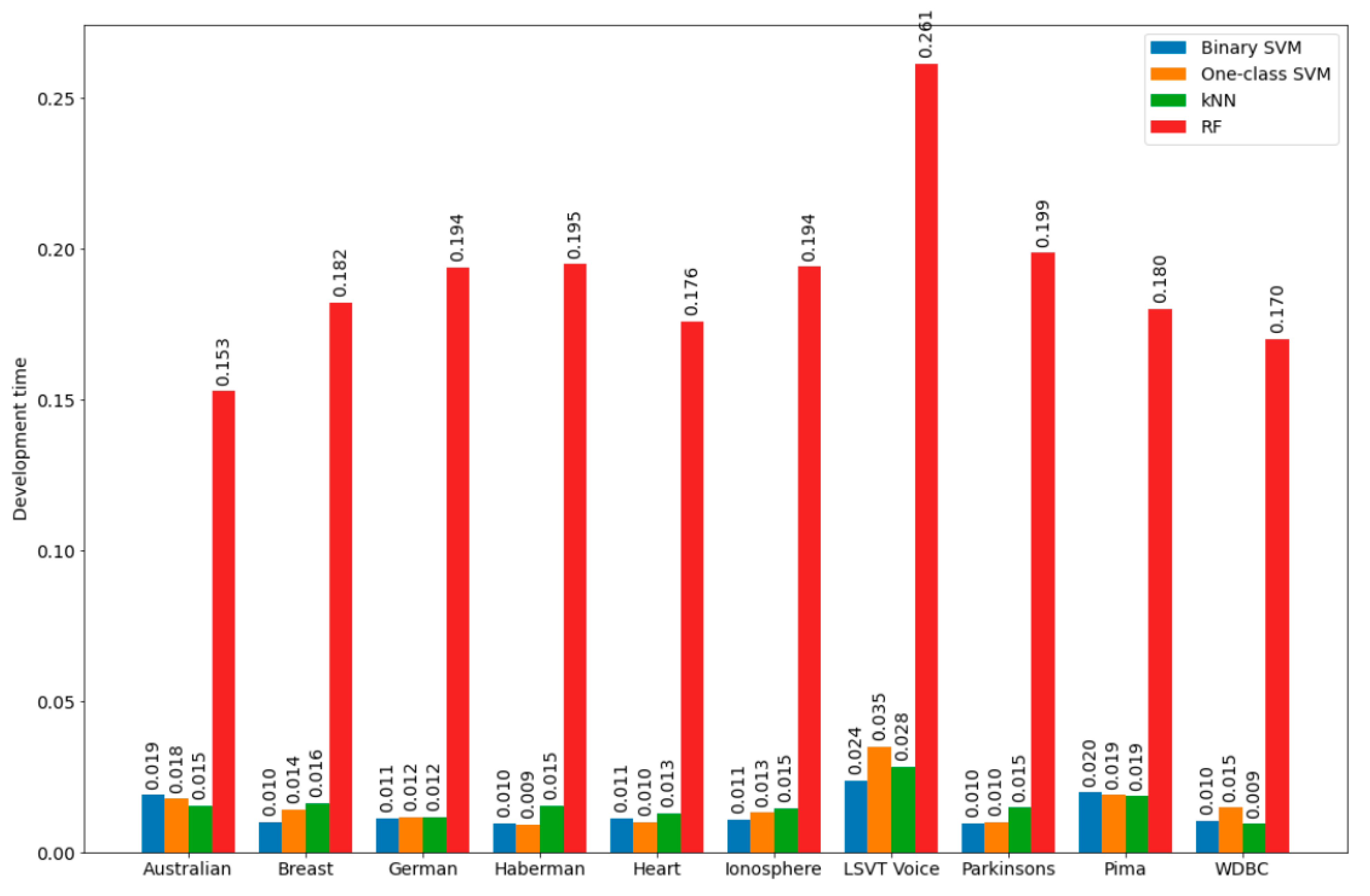
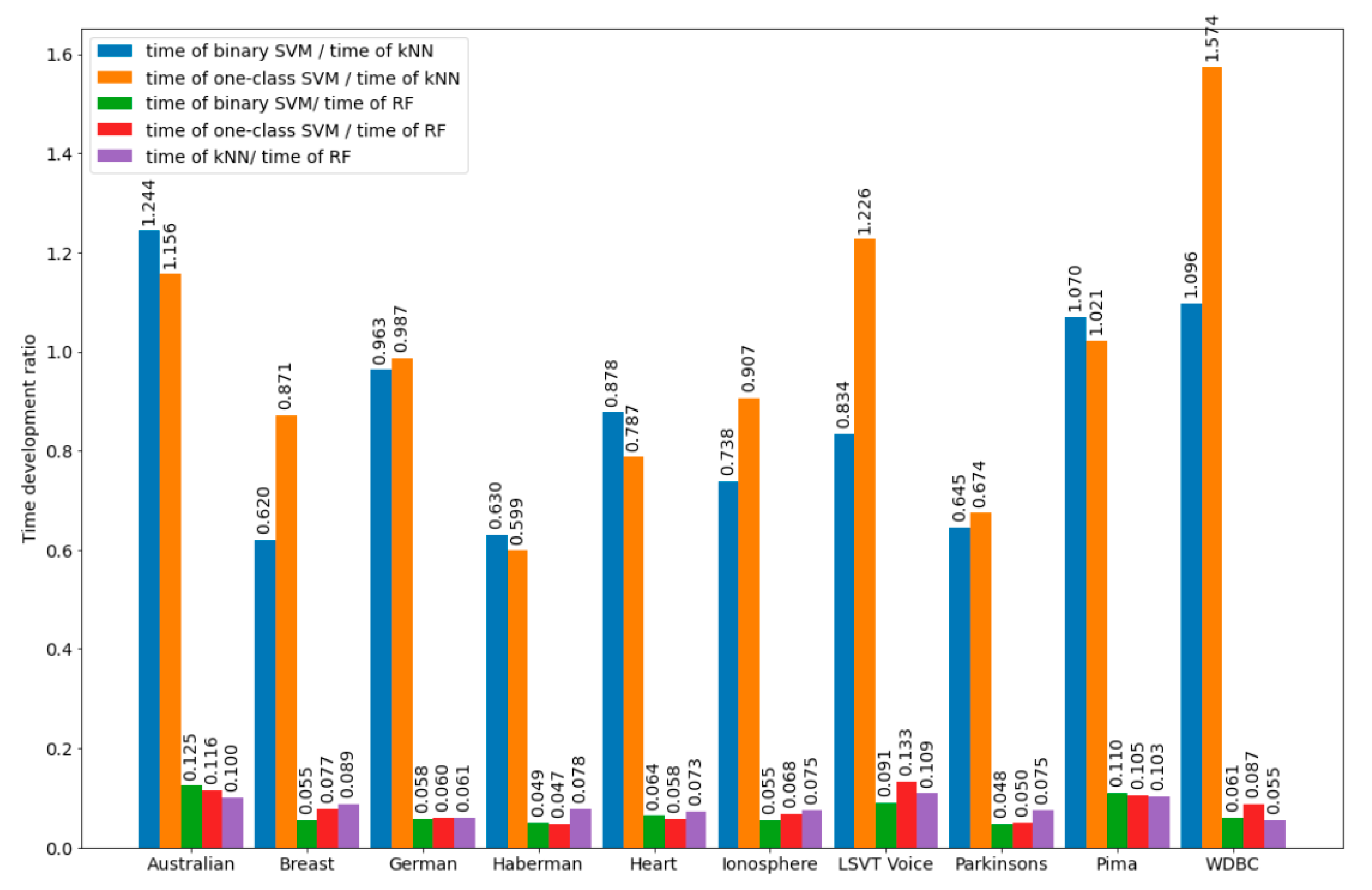
As the results of the experiments have shown, the development time of the kNN classifier was of the same order as the development time of bSVM and obSVM, while the development time of the RF classifier had a higher order. This is why the kNN classifier was chosen as the auxiliary classifier. Figure 2 and Figure 3 show graphical illustrations for the development time of the bSVM, obSVM, kNN, and RF classifiers as well as for the development time ratios for the datasets, the calculated information for which is detailed in Section 5. It can be assumed that approximately the same ratios for the time development will also be in the search for the optimal number of neighbors in the development of the kNN classifier, which is part of the hybrid. Therefore, training of the kNN classifier will be performed on a reduced training set, which should positively affect the development time of the kNN classifier (in the sense of its minimization). It should be noted that the formation time of the reduced training set used in the kNN classifier development was not big and consisted of the time of one pass through the initial training set and the time spent on sorting the objects of the initial training set based on the results of comparing the object class labels in it and the class labels assigned to the same objects by the developed classifier.

The RF classifier can be recommended for use as an auxiliary classifier in a hybrid only if it has significant computing powers (although this classifier, in some cases, allows one to obtain higher classification quality when used both as part of a hybrid and for individual use).

Table 19. Comparative analysis of the classifiers based on accuracy indicator (with Standard scaling).

Classifier/Voting Rule	Haberman/Standard	Heart/Standard	Pima Indians Diabetes/Standard
obSVM-A-kNN/(6)	0.934	-	-
obSVM-B-kNN/(6)	-	0.963	0.870
bSVM-A-kNN/(7)	0.934	-	-
obSVM-A-kNN/(7)	-	0.963	-
obSVM-B-kNN/(7)	-	0.963	-
obSVM-B-kNN/(7)	-	-	0.857
SVM-default	0.918	0.963	0.857
SVM+PSO/-	0.923	0.981	0.857

shows the values of the accuracy indicator assessments obtained for the best two-stage hybrid SVM-kNN classifiers for three datasets (Haberman, Heart, and Pima Indians Diabetes), for which, taking into account various indicators of classification quality, it was possible to prove the effectiveness of the proposed two-stage hybrid SVM-kNN classifiers in comparison with the SVM and kNN classifiers, with parameter values set by default. Table 19 also provides the values of the accuracy indicator parameters values for the binary SVM classifier with default parameter values and the binary SVM classifier built using the modified PSO algorithm [21,22]. The value of the accuracy indicator was estimated using a test dataset. A dash “-” in a table cell means that the classifier specified in the row header was not the best for the dataset specified in the column header. A dash “-” in the last line of the first column means that the voting rule was not applied. The maximum values in the columns are in bold. Analysis of the data in Table 19 allows us to draw the following conclusions. For the Haberman and Pima Indians Diabetes datasets, the proposed two-stage hybrid SVM-kNN classifiers were the best (in the sense of maximizing the value of the accuracy indicator); for the Heart set, the best value of the accuracy indicator was obtained using thee binary SVM classifier built using the modified PSO algorithm. Therefore, we managed to slightly increase the value of the accuracy indicator for the binary SVM classifier built using the modified PSO algorithm compared to the binary SVM classifier with the default parameter values, but we did not manage to exceed the results obtained using the obSVM-A-kNN classifier.

It should be noted that one should pay attention to the time spent on obtaining the best classifiers: How much time is spent on obtaining them? Is it worth spending a lot of time on developing a classifier, or can you obtain a classifier of acceptable quality in less time?

For example, for the Pima Indians Diabetes dataset, the development time for the SVM classifier with default parameter values when the 500 program launches were implemented was approximately 10 s, and the obSVM-B-kNN development time for 500 program launches was approximately 220 s. The development time for the binary SVM classifier using the modified PSO algorithm was approximately 950 s, provided that 500 generations were realized for a population of 60 particles. Each particle determines the parameter values of a certain classifier, during the construction of which one of three types of kernel function (from the list of radial basic, polynomial, and sigmoid kernel functions) is specified, and the parameter values of the kernel function and the regularization parameter value are selected. As we can see, time spent in the latter case turned out to be significantly higher, but at the same time, we could not get the classifier with the highest value of the accuracy indicator. Obviously, when working with large datasets, time spent on developing the binary SVM classifier using the modified PSO algorithm will be even greater, and we will not have a guarantee that we will be able to obtain the desired effective solution.

When using the modified PSO algorithm, it was possible to slightly improve the quality of SVM classifiers for some indicators for three datasets (Australian, German, and Ionosphere); the information on the development of two-stage hybrid SVM-kNN classifiers is given in Table A2, Table A3, Table A4, Table A5, Table A6 and Table A7. However, the question arises again regarding the expediency of significant time expenditures to obtain the desired solution.

Obviously, a reasonable approach would be to implement the development process for two-stage hybrid versions of SVM-kNN classifiers with the choice of the best classifier from all available at the current launch of the program.

The impossibility of obtaining an effective solution using aa two-stage hybrid of the SVM-kNN classifier for some datasets may be due to the fact that it was not possible to provide the necessary rebalancing of classes within the strip separating them. In addition, it can be caused by the specifics of grouping objects within the strip separating the classes.

It should be noted that the development process of two-stage hybrid SVM-kNN classifiers can be parallelized, which can be very important when working with big data.

7. Conclusions

In general, the obtained results allow us to speak about the prospects of using two-stage hybrid SVM-kNN classifiers with the aim to increase the data classification quality.

In the course of further research, it is planned to investigate the possibility of using, as an additional toolkit, classifiers such as kNN classifiers that implement various weighted options to account for the nearest neighbors and perform a quick search for the nearest neighbors, classifiers based on the Parzen window algorithm, RF classifiers, etc. In addition, it is of considerable interest to analyze the influence of the choice of symmetric and asymmetric areas within the boundaries defining the hyperplane dividing the classes when forming the training and test subsets for the kNN classifier on the overall quality of the classifier.

The proposed two-stage hybrid SVM-kNN classifier is fundamentally different from the hybrid SVM-kNN classifier proposed in [52,53] by the method of forming a training set for the developing kNN classifier: in [52,53], objects were used that lie outside the area, which, moreover, can be formed taking into account the principles of symmetry and asymmetry with respect to the hyperplane dividing the classes, and the proposed study used objects lying inside the area formed based on the principles of symmetry with respect to the hyperplane dividing the classes. Similar principles (as in [52,53]) for the formation of a training set were considered in [68,69]. Therefore, we plan to research the opportunity of using two versions of one-class SVM-algorithm—ooSVM and obSVM—for the development of the concept of the hybrid SVM-kNN classifier proposed in [52,53]. Therefore, the main problem in all two-stage hybrid SVM-kNN classifiers is the problem of applicability of the kNN classifier at the second stage, due to the possible small number of objects in the reduced training set formed using the results from the SVM classifier development.