Abstract
To improve fire prediction accuracy over existing methods, a double weighted naive Bayes with compensation coefficient (DWCNB) method is proposed for fire prediction purposes. The fire characteristic attributes and attribute values are all weighted to weaken the assumption that the naive Bayes attributes are independent and equally important. A compensation coefficient was used to compensate for the prior probability, and a five-level orthogonal testing method was employed to properly design the coefficient. The proposed model was trained with data collected from the National Institute of Standards and Technology (NIST) fire database. Simulation comparisons show that the average prediction accuracy of the proposed method is 98.13%, which is 5.08% and 2.52% higher than the methods of naive Bayes (NB) and double weighted naive Bayes (DWNB), respectively. The experimental results show that the average accuracies of the DWCNB method for test fire and interference sources were 97.76% and 98.24%. Prediction accuracies were 5.06% and 3.74% higher than those of the NB and DWNB methods.
1. Introduction
Urban fires are notable threats to the safety of human lives and property. According to the National Fire Protection Association (NFPA) research report, in 2018, US fire departments responded to an estimated 1,318,500 fires that together caused 3655 civilian deaths and estimated losses of $25.6 billion [1]. With fast population growth and the large-scale use of electrical appliances, potential fire threats are increasing. Efficiently collecting environmental data and correctly predicting potential fire accidents are particularly important to preventing deaths and damage from fire accidents [2].
Environmental parameters can change suddenly before the actual occurrence of an accidental fire. Such parameters include the temperature, humidity, carbon monoxide concentration, carbon dioxide concentration, and smoke concentration. Collecting such parameters and predicting fires is an effective way to stop fire accidents.
A home fire alarm system was developed in [3] based on the temperature detection method. The ambient temperature was detected and the alarm was triggered when the temperature was above 40 °C. In the work by Jiang et al. [4], a compound fire alarm system for detecting smoke particles and carbon monoxide was designed on the basis of the photoacoustic spectrometry principle. The CO concentration and extinction coefficient of smoke particles were measured, and a compound value was developed as the alarm criterion. Implementation of these methods is usually simple. However, the prediction accuracy is largely dependent on the threshold value. In a complex environment, false or missed alarms could occur if the threshold is not properly designed.
Image recognition is another method that has been studied for fire prediction [5,6,7]. After some basic processes, including image acquisition, image processing, and feature extraction, fire accidents could be identified by properly designed classifiers, and thus early fire warnings could be provided. However, this method is sensitive to environmental disturbances, such as fog and strong light. Additionally, for environments with few stand-out features, feature extraction and observation are usually difficult. To increase fire prediction’s accuracy and stability, intelligent artificial-based algorithms are being studied. The design and development of a fuzzy logic-based multi-sensor fire detection system was discussed in [8]. A multi-sensor approach was employed whereby the outputs of three sensors, sensing three different fire signature parameters (smoke, flame, and temperature), contributed to the fire alert decision; this was a more reliable fire detection system, devoid of false alarms.
Neural network algorithms [9,10,11] have also been used in early fire warnings. They have strong anti-interference, high fault tolerance, and high system reliability. However, a neural network usually requires a large number of parameters, such as initial values of network topology, different weights, and thresholds. Proper design and collection of such parameters is difficult. Additionally, implementing a neural network requires a large number of calculations, and usually results in very high hardware costs.
The naive Bayes (NB) algorithm is a classification method based on probability theory. The working principle is simple and easy to implement, with moderate costs. With reasonable improvements, the prediction results could be accurate and stable, and they have been widely used in applications such as spam email classification [12], text emotion analysis [13], and fire prediction [14]. The ability to deal with uncertain evidence can be used in fire warning prediction. The NB algorithm is based on the assumption that naive Bayesian attributes are independent and equally important, which is usually unsatisfied in reality and needs to be improved. In [15], a term weighting scheme was proposed in which the weight of each term was dependent on its semantic similarity to the text category. This method improved the algorithm’s performance by counting the word frequency in the text and determining the weighting coefficient. Jiang et al. [16] applied the depth feature weighting method to improve the naive Bayes algorithm. To increase accuracy and efficiency, they proposed incorporating the learned weights into both the formula of classification and its conditional probability estimates. These improvements were useful to obtain better solutions for text categorization compared to the normal NB method. However, the method takes the frequency of the characteristic attribute as the basis to determine the weight. The inter-class attribute distribution relationship is not considered. A similar depth feature weighting method was discussed in [17] to improve the algorithm. The correlation-based feature selection (CFS) method was employed to determine the weighting coefficients. The weighting coefficients corresponding to selected and unselected characteristic attributes were set as 2 and 1, respectively. This design is able avoid the influence of the frequency distribution of characteristic attributes, but still the correlation between decision categories and samples is not considered.
In [18], two improved NB algorithms were proposed to improve the imbalance problem of positive and negative classification accuracy. The influences of the characteristic attributes’ frequency and the attributes’ values were considered in the two improvements. However, in the weighting decision process, the weights were directly chosen as constants of 0.00001 and 0.99999, instead of calculating the weights based on the sample. Reflection of the characteristic attributes is insufficient in the decision-making process.
To solve these problems, a double weighted naive Bayes with the compensation coefficient (DWCNB) method is proposed for fire prediction purposes. The main contributions of this study can be summarized as follows: (1) The double weighted naive Bayes with compensation coefficient method is proposed for fire prediction. (2) The characteristic attributes of fire and the attribute values are both weighted to weaken the naive Bayes’ attribute assumptions of independence and equal importance. (3) A compensation coefficient is used to compensate for the prior probability, and a five-level orthogonal testing method was employed to properly design the compensation coefficient based on the samples. The attributes of temperature, smoke concentration, and carbon monoxide concentration were integrated. Based on the improved classification model, three decisions are provided, including open flame (OF), smoldering fire (SF), and no fire (NF). The sample library is described with a three-dimensional vector group {r s t}, where r represents the sample number, s is the number of the characteristic vectors, and each characteristic vector has t values. To consider the relationships among characteristic attributes, the weight of the characteristic attribute is determined by sample fluctuations and the content. By considering the connection among the characteristic attributes, the weight value is determined by the frequency of the characteristic attribute value. At the same time, the prior probability compensation is employed to reduce the importance of weighting, and thus weaken the assumption that naive Bayesian attributes are independent and equally important, to improve prediction accuracy. This paper is organized as follows. The principle of the naive Bayesian classifier is discussed in Section 2. The proposed model and the improvements of the naive Bayesian algorithm are demonstrated in Section 3. In Section 4, the platform implementation and the simulation comparisons between different methods are discussed. Experimental verifications and conclusions are given in Section 5 and Section 6, respectively.
2. Naive Bayesian Classifier
The naive Bayesian method was developed based on Bayesian decision theory. The prior probability and conditional probability parameters are obtained from prior knowledge, and then the posterior probability distribution is calculated with the Bayesian formula, and the probability of certain category belongings can be predicted by comparing the probabilities. The basic model is [19]
where represents probability. Here, we assume each fire dataset has n characteristic attributes and m decision categories . Since takes the same value for each decision category, according to the conditional independence assumption, the naive Bayesian classification model [19] can be obtained as
where is the prior probability of the decision category , and is the conditional probability that the characteristic attribute is and the decision category is . For a certain dataset to be classified as , the prior probability is obtained from the dataset. The product of the conditional probability of each characteristic attribute is calculated under each decision category . Then, the priori probability and the conditional probability are multiplied to obtain the posterior probability . The class with the largest posterior probability is then taken as the class to which the object belongs.
3. Practical Enhancements in the Naive Bayesian Algorithm to Augment Fire Prediction Accuracy
3.1. Laplace Smoothing
When implementing the naive Bayesian algorithm, it is necessary to calculate the product of multiple probabilities . to obtain the classification probability. If one of the probabilities is 0, which means the total value of the characteristic attribute is 0, then the test data can never be classified. This phenomenon is usually observed when the number of samples in a training set is too small to satisfy the large numbers law [20].
To solve this problem, Laplace smoothing can be used by initializing the value of each characteristic to be 1. When the training samples are large enough, the frequency of each characteristic attribute is increased by 1 and the effect of the final classification value is negligible. In this case, the zero probability problem can be effectively solved. After Laplacian smoothing, the conditional probability that a characteristic attribute with value , is calculated as
where is the frequency of the decision category , and is the frequency that the characteristic attribute takes the value of and belongs to the decision category , and is the number of all the values of the characteristic attribute .
3.2. Logarithmic Operation
The probabilities need to be multiplied together to get . The underflow problem could be induced if the probabilities are too small. To avoid this, the logarithmic operation can be employed to turn multiplication into addition. The same monotonicity and the extremum of the two calculations ensure the final classification result is not affected. The logarithmic operation of (2) gives the following naive Bayesian classification model:
It can be seen from (4) that the classification calculation has been turned from multiplication into addition, and the underflow problem can be avoided.
3.3. Double Weighting of Characteristic Attribute
The naive Bayesian classification model is based on the assumption that the attribute values are independent from each other under the conditions of each classification feature. Each characteristic attribute has the same decision-making importance as the others in its corresponding category. However, in practice, these assumptions are difficult to satisfy [21]. Weighting different characteristic attributes with proper weighted coefficients is one of the ways to weaken this assumption. In this paper, a double weighted naive Bayes with the compensation coefficient (DWCNB) method is proposed. Weighting both characteristic attributes and characteristic attribute values weakens the assumption that the naive Bayesian attributes are independent and equally important. The improved classification model is
where is the weight coefficient of the characteristic attribute under the decision category ; is the weight coefficient of the characteristic attribute with the value of under the decision category . The calculation formula of the characteristic attribute weighting coefficient is
where is the variance of the characteristic attribute under the decision category , and is the sum of the variances of all characteristic attributes under the decision category. , is the variance contribution rate of the characteristic attribute to the decision category , and is the average value of the characteristic attribute under the decision category , representing the influence of the characteristic attribute’s content on the decision category.
The calculation formula of the characteristic attribute value weighting coefficient is
where is the frequency of the decision category , and is the frequency of the characteristic attribute with the value of under the decision category .
3.4. Prior Probability Compensation
It can be seen from the naive Bayesian classification model (2) that the classification result is determined by both the prior probability and the conditional probability . The weighting of the characteristic attributes and the characteristic attribute values in (5) only applies to the conditional probability, which could lead to an unbalanced decision-making effect on the classification result. This unbalanced decision-making effect could be magnified after the logarithm operation, resulting in incorrect classification results. To improve accuracy, it is proposed that the different decision categories, , are compensated by introducing a prior probability compensation coefficient to balance the decision-making effect of the prior probability part and the conditional probability part. The classification model after prior probability compensation can be written as
After compensation, the influence caused by the uneven distribution of sample data categories can be reduced. The value of can be designed from proper experimental testing; this will be discussed later.
4. Fire Prediction Model
4.1. Development of the Classification Model
Three variables were chosen as the characteristic attributes in the classification model: temperature, smoke concentration, and carbon monoxide concentration. Three decision categories were defined: open flame (OF), smoldering fire (SF), and no fire (NF). To verify the model, the dataset from the National Institute of Standards and Technology Report (Fire Research Division) [22] was selected, including 12 tests and 4972 fire datasets. The 12 selected tests involved four different materials: wood, cotton rope, polyurethane plastic, and ethanol. In each test, the status of OF, SF, and NF were included. Part of the dataset after normalization is shown in Table 1. We selected 15 instances for the table. For each instance, there are three data points and a corresponding fire category. The three data points represent the values of temperature, smoke concentration, and carbon monoxide concentration.

Table 1.
Partial fire data.
The prediction model was implemented with Python, and the specific calculation steps are shown in Figure 1.
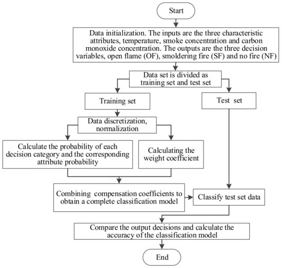
Figure 1.
Training and testing flowchart of the model.
In Figure 1, details of the numerical implementation and calculation procedures are described by the following five methodological steps:
- (1)
- Divide the dataset into two groups: the training set and the test set. Data preprocessing is applied, including data discretization and normalization.
- (2)
- Based on the samples from the training set, calculate the probability of the decision category , and the conditional probability of the characteristic attribute with the value of under the decision category .
- (3)
- Calculate the characteristic attribute weighting coefficient and the characteristic attribute value weighting coefficient according to (6) and (7), respectively.
- (4)
- Determine the prior probability compensation coefficient. The decision category model is developed based on the weighting of characteristic attributes, and a complete weighted naive Bayes classifier is obtained.
- (5)
- For data point Y to be classified, apply the developed naive Bayes classifier to classify the data.
4.2. Determination of the Compensation Coefficient
In this paper, we propose compensating for the different decision categories by introducing a prior probability compensation coefficient . An orthogonal test method was developed to properly design . The accuracy rate A is defined as an evaluation index, which is expressed as
where denotes the total number of data points that can be correctly identified as open flames, smoldering fire, or no fire; and is the total number of data points in the test set. Assume that there are three factors for in the first orthogonal test: , , and . According to the empirical level, each factor has four values, 1.5, 2.5, 3.5, and 4.5, which can be used in 3-factor and 4-level orthogonal tests. The orthogonal table was selected as L16(43) to construct the preliminary determination test for . The test results are shown in Table 2.
Table 2.
L16(43) orthogonal test results.
It can be seen from Table 2 that the classification accuracy is largely affected by , and the influence from is relatively small. The optimal level of is 1, so the initial value of was set as 1.5. The optimal level of is 2 and the initial value of was 2.5. The optimal level of is 3 and the initial value of was 3.5.
Based on the results of L16(43), the second orthogonal test was conducted to determine the final value of . Three factors, , , and , were chosen. Each factor was divided into five levels, for 3-factor and 5-level orthogonal tests. The orthogonal table was selected as L25 (53). The factor level and the test results are shown in Table 3 and Table 4.
Table 3.
Factor levels.
Table 4.
L25(53) orthogonal test results.
It can be seen from Table 4 that the classification accuracy of the classification model is still largely dependent on . The influence from is still small. The optimal levels of , , and are 1, 4, and 2, respectively. Therefore, it can be determined that the values are = 1.1, = 2.7, = 3.3.
4.3. Classification Model Performance Analysis
For a two-class classification problem, with negative (class 0) and positive (class 1) classes, the confusion matrix shown in Table 5 is needed to analyze the model’s performance. By using the definitions in Table 5, the proposed classification model was evaluated with three indexes: the precision , the recall , and the F-measure . Precision is a metric that quantifies the number of correct positive predictions made. Precision, therefore, calculates the accuracy for the minority class. It is calculated as the ratio of correctly predicted positive examples divided by the total number of positive examples that were predicted. Recall is a metric that quantifies the number of correct positive predictions made out of all positive predictions that could have been made. Unlike precision, which only comments on the correct positive predictions out of all positive predictions, recall provides an indication of missed positive predictions.
Table 5.
The confusion matrix.
There are three categories in our model: open flame (OF), smoldering fire (SF), and no fire (NF). To conduct the evaluation, OF, SF, and the total fire status (TF, summation of OF and SF) were evaluated, with the three indexes calculated with the following formulae:
We calculated the three indexes of three different models: the naive Bayesian algorithm (NB), the double-weighted naive Bayesian algorithm (DWNB), and the proposed DWCNB algorithm. We followed the procedure introduced in [19] to develop the NB classifier. Weighted naive Bayes methods have been discussed in [16,17], and have been successfully used in text classification. The DWNB method was developed by using a similar idea for fire prediction purposes. The fire characteristic attributes and attribute values are both weighted.
In the proposed DWCNB method, the compensation coefficient was calculated according to the procedures demonstrated in Section 3.2. A total of 2984 data samples in the NIST database were selected as the training set, and 1988 data samples were used as the test set. The frequency of each category was counted, and the calculation of each index was performed. The test results are shown in Figure 2. It can be seen from Figure 2 that, with the improvement of double weighting and the coefficient compensation, the indexes of the three states, OF, SF and TF, of the DWCNB can achieve high values of around 96%. The recall rate of SF was up to 97.35%, which was much higher than the SF of NB and DWNB. Since the characteristic attribute weights and the corresponding influences on category decision results were considered, compared with NB, the three indexes of TF increased by 5.89%, 4.59%, and 5.25%. Compared with DWNB, the increased rates of TF were 2.2%, 2.8%, and 2.25%. The improvements came from the consideration of the decision-making effect of each characteristic attribute, corresponding to different decision categories. The relationship between characteristic attributes is considered. By introducing the weights, the influence of different values of each characteristic attribute on the classification performance under each decision category is described. Additionally, the decision-making effects of the prior and conditional probabilities can be balanced via the proposed compensation coefficients. It can also be seen from Figure 2 that, for the TF state, the recall rates of the three methods are larger than the precision rates. In practice, we hope that the false negative results can be reduced. We would rather report false positives than false negatives (missed alarms) in a strong interference environment, and these simulation results are consistent with practical demands.
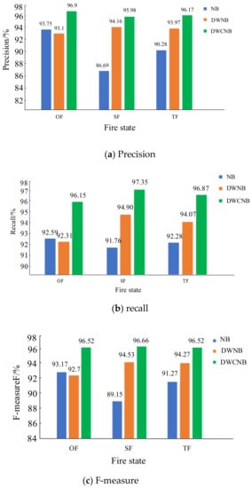
Figure 2.
Model simulation results before and after improvement.
By using the definition in (9), the prediction accuracies of the three methods were compared. A total of 3480 data points were randomly selected from the NIST database for verification. Comparison results are shown in Table 6. It can be seen from Table 6 that the prediction accuracy demonstrated small changes for different test sets. Compared with NB, after introducing double weighting, the average accuracy increase of DWNB was 2.56%. The proposed DWCNB had the highest accuracy, which was 5.08% and 2.52% higher than NB and DWNB.
Table 6.
Simulation results of the model.
5. Experimental Verification
The hardware design was based on the STM32L151 chip (Figure 3a). The proposed DWCNB algorithm was implanted into the embedded system, and a combustion chamber (Figure 3b) was employed for the experimental verification. As shown in Figure 3a, the characteristic signals, including temperature, smoke concentration, and carbon monoxide concentration, were collected with the corresponding temperature sensor DHT11, the smoke sensor MQ-2, and the carbon monoxide sensor MQ-7. The sampling frequency was 166.67 kHz. After pre-processing, the characteristic signals were measured and three indicator lights of red, yellow, and green were used to indicate different prediction results, corresponding to open flame, smoldering fire, and no fire states. A buzzer was used for the open flame and smoldering fire states. The complexity of the proposed algorithm’s implementation and hardware design was relatively simple compared with intelligent artificial-based platforms. However, we needed to run the five-level orthogonal test to determine the coefficients, and it required some work to set up the whole platform.
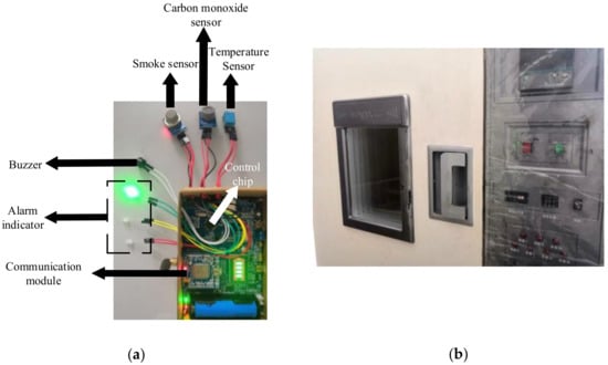
Figure 3.
Experimental setup.
Different materials, including wood, cotton rope, polyurethane plastic, and ethanol, were selected as the combustion materials. The fire states were set as wood smoldering fire, cotton rope smoldering fire, polyurethane plastic open flame, and ethanol open flame. A total of 1500 datasets were collected for each test fire, and the accuracy was calculated based on (9). The experimental results are shown in Table 7. It can be seen from Table 7 that for different test fires, the accuracies of DWNB were higher than those of NB. There were small accuracy differences between the different test fires. The proposed DWCNB method demonstrated the highest accuracies. The average accuracy was 5.06% and 3.74% higher than the accuracies of NB and DWNB methods, respectively.
Table 7.
Accuracy of the test fires.
Experimental verification of interference sources was also conducted. Cigarette lighters, dust, and cigarette smoke were taken as the interference sources of the no-fire state. A total of 1500 datasets were collected for each interference source, and the prediction accuracy is shown in Table 8. It can be seen from the table that the DWCNB method has a relatively higher anti-interference ability compared with NB and DWNB. The average accuracy was 98.24–5.11% and 2.95% higher than NB and DWNB, respectively. Additionally, the prediction accuracy of DWCNB against dust interference was the largest (99.47%). Accuracies against cigarette smoke interference were the lowest for all three methods, which means interference from the cigarette smoke was most severe among the three sources.
Table 8.
Accuracy against the interference source.
The hardware platform was developed based on the STM32L151 chip with three external sensors: the temperature sensor, the smoke sensor, and the carbon monoxide sensor. Implementation and installation of the device was simple. With the embedded DWCNB algorithm, it was able to provide a simple and accurate solution for early fire prediction.
6. Conclusions
An improved naive Bayes algorithm for fire prediction was developed in this study. Verification showed that the average prediction accuracies of the proposed method were 5.06% and 3.74% higher than those of NB and DWNB methods, respectively. The average accuracy against the interferences of DWCNB was 98.24%, which was 5.11% and 2.95% higher than those of NB and DWNB, respectively. In our study, different materials, including wood, cotton rope, polyurethane plastic, and ethanol, were selected as the combustion materials. In the future, different materials could be used to further verify the method. Additionally, it would be interesting to explore other strategies to determine the compensation coefficient used in the prior probability calculations.
Author Contributions
Conceptualization, L.S.; methodology, H.Z.; software, Y.Y.; validation, Y.C. and W.C.; formal analysis, Y.Y.; investigation, L.S.; resources, H.Z.; data curation, H.Z.; writing—original draft preparation, L.S.; writing—review and editing, Y.Y.; visualization, H.Z.; supervision, L.S. All authors have read and agreed to the published version of the manuscript.
Funding
This research was funded by National Natural Science Foundation of China (51507113), the Zhejiang Public Welfare Technology Research Plan (LGC20E070001), the project of Zhejiang Provincial Department of Education (Y201737046) and the Major Scientific and Technological Innovation and Key Industrial Projects in Wenzhou city (ZG2019017).
Conflicts of Interest
The authors declare no conflict of interest.
Nomenclature
| Probability | |
| Characteristic attribute | |
| Categories | |
| Number of all the values of the characteristic attribute | |
| Variance of the characteristic attribute under the decision category | |
| Average value of the characteristic attribute under the decision category | |
| Prior probability compensation coefficient | |
| Total number of data that can be correctly identified for open flame, smoldering fire and no fire | |
| Total number of data in the test set | |
| True Positive | |
| False Positive | |
| True Negative | |
| False Negative | |
| Double weighted naive Bayes with compensation coefficient | |
| Double weighted naive Bayesian algorithm | |
| Naive Bayes | |
| Basic naive Bayesian model | |
| Naive Bayesian classification model | |
| Characteristic attribute weighting coefficient | |
| Weight coefficient of the characteristic attribute value under the decision category | |
| Accuracy rate | |
| Accuracy rate of model | |
| Recall rate | |
| F-measure |
References
- National Fire Protection Association. Fires in the U.S. Available online: http://www.nfpa.org/research/reports-and-statistics/fires-in-the-us (accessed on 27 November 2019).
- Ayala, P.; Cantizano, A.; Sánchez-Úbeda, E.F.; Gutiérrez-Montes, C. The Use of Fractional Factorial Design for Atrium Fires Prediction. Fire Technol. 2017, 53, 893–916. [Google Scholar] [CrossRef]
- Mahzan, N.N.; Enzai, N.I.M.; Zin, N.M.; Noh, K.S.S.K.M. Design of an Arduino-based home fire alarm system with GSM module. J. Phys. Conf. Ser. 2018, 1019, 12079. [Google Scholar] [CrossRef]
- Jiang, Y.L.; Li, G.; Wang, J.J. Photoacoustic compound fire alarm system for detecting particles and carbon monoxide in smoke. Fire Technol. 2016, 52, 1255–1269. [Google Scholar] [CrossRef]
- Wang, S.; He, Y.; Zou, J.; Duan, B.; Wang, J. A Flame Detection Synthesis Algorithm. Fire Technol. 2014, 50, 959–975. [Google Scholar] [CrossRef]
- Chunyu, Y.; Jun, F.; Jinjun, W.; Yongming, Z. Video fire smoke detection using motion and color features. Fire Technol. 2010, 46, 651–663. [Google Scholar] [CrossRef]
- Xu, G.; Zhang, Q.; Zhang, Y.; Lin, G.; Wang, J.; Wang, Z. Video smoke detection based on deep saliency network. Fire Saf. J. 2019, 105, 277–285. [Google Scholar] [CrossRef]
- Sowah, R.A.; Ofoli, A.R.; Krakani, S.N.; Fiawoo, S.Y. Hardware Design and Web-Based Communication Modules of a Real-Time Multisensor Fire Detection and Notification System Using Fuzzy Logic. IEEE Trans. Ind. Appl. 2017, 53, 559–566. [Google Scholar] [CrossRef]
- Luo, Y.; Zhao, L.; Liu, P.; Huang, D. Fire smoke detection algorithm based on motion characteristic and convolutional neural networks. Multimed. Tools Appl. 2018, 77, 15075–15092. [Google Scholar] [CrossRef]
- Mao, W.; Wang, W.; Dou, Z.; Li, Y. Fire Recognition Based On Multi-Channel Convolutional Neural Network. Fire Technol. 2018, 54, 531–554. [Google Scholar] [CrossRef]
- Wu, D.; Wu, H.; Zhao, J. An intelligent fire detection approach through cameras based on computer vision methods. Process Saf. Environ. Prot. 2019, 127, 245–256. [Google Scholar] [CrossRef]
- Ebadati, O.M.E.; Ahmadzadeh, F. Classification Spam Email with Elimination of Unsuitable Features with Hybrid of GA-Naïve Bayes. J. Inf. Knowl. Manag. 2019, 18. [Google Scholar] [CrossRef]
- Tago, K.; Takagi, K.; Kasuya, S.; Jin, Q. Analyzing influence of emotional tweets on user relationships using Naïve Bayes and dependency parsing. World Wide Web 2019, 22, 1–16. [Google Scholar] [CrossRef]
- Kern, A.N.; Addison, P.; Oommen, T.; Salazar, S.E.; Coffman, R.A. Machine learning based predictive modeling of debris flow probability following wildfire in the intermountain western United States. Math. Geosci. 2017, 49, 717–735. [Google Scholar] [CrossRef]
- Luo, Q.; Chen, E.; Xiong, H. A semantic term weighting scheme for text categorization. Expert Syst. Appl. 2011, 38, 12708–12716. [Google Scholar] [CrossRef]
- Jiang, Q.; Wang, W.; Han, X.; Zhang, S.; Wang, X.; Wang, C. Deep feature weighting in Naïve Bayes for Chinese text classification. In Proceedings of the 2016 4th IEEE International Conference on Cloud Computing and Intelligence Systems, CCIS, Beijing, China, 17–19 August 2016; pp. 160–164. [Google Scholar]
- Jiang, L.; Li, C.; Wang, S.; Zhang, L. Deep feature weighting for Naïve Bayes and its application to text classification. Eng. Appl. Artif. Intell. 2016, 52, 26–39. [Google Scholar] [CrossRef]
- Kang, H.; Yoo, S.J.; Han, D. Senti-lexicon and improved Naïve Bayes algorithms for sentiment analysis of restaurant reviews. Expert Syst. Appl. 2012, 39, 6000–6010. [Google Scholar] [CrossRef]
- Han, J.; Kamber, M.; Pei, J. Data Mining: Concepts and Techniques; Elsevier: Amsterdam, The Netherlands, 2012. [Google Scholar]
- Arar, Ö.F.; Ayan, K. A feature dependent Naïve Bayes approach and its application to the software defect prediction problem. Appl. Soft Comput. 2017, 59, 197–209. [Google Scholar] [CrossRef]
- Jiang, L.; Zhang, L.; Yu, L.; Wang, D. Class-specific attribute weighted Naïve Bayes. Pattern Recognit. 2019, 88, 321–330. [Google Scholar] [CrossRef]
- Richard, W.B.; Richard, D.P.; Jason, D.A. Performance of Home Smoke Alarms Analysis of the Response of Several Available Technologies in Residential Fire Settings; U.S. Government Printing Office: Washington, DC, USA, 2008.


Publisher’s Note: MDPI stays neutral with regard to jurisdictional claims in published maps and institutional affiliations. |
© 2021 by the authors. Licensee MDPI, Basel, Switzerland. This article is an open access article distributed under the terms and conditions of the Creative Commons Attribution (CC BY) license (http://creativecommons.org/licenses/by/4.0/).