Article

An Improved SPSIM Index for Image Quality Assessment

Department of Data Science and Engineering, Silesian University of Technology, Akademicka 16, 44-100 Gliwice, Poland
*
Author to whom correspondence should be addressed.
Symmetry 2021, 13(3), 518; https://doi.org/10.3390/sym13030518
Submission received: 4 February 2021 / Revised: 15 March 2021 / Accepted: 18 March 2021 / Published: 22 March 2021

Abstract

:
Objective image quality assessment (IQA) measures are playing an increasingly important role in the evaluation of digital image quality. New IQA indices are expected to be strongly correlated with subjective observer evaluations expressed by Mean Opinion Score (MOS) or Difference Mean Opinion Score (DMOS). One such recently proposed index is the SuperPixel-based SIMilarity (SPSIM) index, which uses superpixel patches instead of a rectangular pixel grid. The authors of this paper have proposed three modifications to the SPSIM index. For this purpose, the color space used by SPSIM was changed and the way SPSIM determines similarity maps was modified using methods derived from an algorithm for computing the Mean Deviation Similarity Index (MDSI). The third modification was a combination of the first two. These three new quality indices were used in the assessment process. The experimental results obtained for many color images from five image databases demonstrated the advantages of the proposed SPSIM modifications.

1. Introduction

Quantitative domination of acquired color images over gray level images results in the development not only of color image processing methods but also of Image Quality Assessment (IQA) methods. These methods have an important role in a wide spectrum of image processing operations such as image filtration, image compression and image enhancement. They allow an objective assessment of the perceptual quality of a distorted image. Distorted images do not necessarily originate from the image acquisition process but can be created by various types of image processing. Among IQA methods, the most developed are methods that compare the processed (distorted) images to the original ones, and are called Full-Reference IQA (FR-IQA) methods. In this way, they assess the image quality after performing image processing operations. The assessments obtained for each IQA measure can be compared with the subjective Mean Opinion Score (MOS) or Difference Mean Opinion Score (DMOS) average ratings from human observers. However, determining subjective MOS values is time-consuming and expensive. In many practical applications, the reference image is unavailable, and therefore “blind” IQA techniques are more appropriate. When we use the FR-IQA methods then the results of comparisons will be the correlation coefficients: the higher the number, the better the measure. In conclusion, the aim of research in the field of IQA is to find measures to objectively and quantitatively assess image quality according to subjective judgment by a Human Visual System (HVS). There is a tradition in the IQA field of improving and refining existing quality measures. Similarly, attempts are made to assemble elements of one measure with elements of another measure to increase the correlation of the index with the MOS.
A low-complexity measure named the Mean Squared Error (MSE) has dominated for a long time among IQA measures used in color image processing due to its simplicity. Similarly popular was the use of other signal-theory-based measures such as Mean Absolute Error (MAE) and Peak Signal-to-Noise Ratio (PSNR). Over time, a weak link has been noted between these measures and human visual perception. The work [1] shows the drawback in the PSNR measure using the example of the Lighthouse image. Additional noise was added to this image and its copy and was located in the lower or upper part of the image. In the first case the noise was invisible to the observer; in the second case it reduced the image quality assessment. Meanwhile, the PSNR values for both images were the same. Comparison of images on a pixel-to-pixel basis does not allow the influence of the pixel’s neighborhood on the perceived color. This lack of influence is a disadvantage for all those the measures mentioned above.
Since 2004, the Structural Similarity Index Measure (SSIM) [2] has been used as an IQA method, which reflects the perceptual change of information about the structure of objects in a scene. This measure uses the idea of pixel inter-dependencies, which are adjacent to each other in image space. The SSIM value in compared images is created as a combination of three similarities of luminance, contrast and structure. It is calculated by averaging the results obtained in separate local windows (e.g., 8 × 8 or 11 × 11 pixels). In 2011, the Gradient SIMilarity index measure (GSIM) [3] was proposed to consider the similarity of the gradient in images by expressing their edges. These ideas have thus become a starting point for new perceptual measures of image quality and many such IQA measures were proposed during the last decade. In [4], a quality index named the Feature SIMilarity index (FSIM) was proposed. Here the local quality of an evaluated image is described by two low-level feature maps based on phase congruency (PC) and gradient magnitude (GM). FSIMc, a color version of FSIM, is a result of IQ chrominance components incorporation. Another example of a gradient approach is a simple index called the Gradient Magnitude Similarity Deviation (GMSD) [5]. The gradient magnitude similarity map expresses the local image quality and then the standard deviation of this map is calculated and used as the final quality index GMSD.
Zhang L. et al. [6] described a measure named the Visual Saliency-based Index (VSI), which uses a local quality map of the distorted image based on saliency changes. In addition, visual saliency serves as a weighting function conveying the importance of particular regions in the image.
Recently, Nafchi et al. [7] proposed new IQA model named the Mean Deviation Similarity Index (MDSI), which uses a new gradient similarity for the evaluation of local distortions and chromaticity similarity for color distortions. The final computation of the MDSI score requires a pooling method for both similarity maps; here a specific deviation pooling strategy was used. A Perceptual SIMilarity (PSIM) index was presented in [8], which computed micro- and macrostructural similarities, described as usual by gradient magnitude maps. Additionally, this index uses color similarity and realizes perceptual-based pooling. IQA models developed recently are complex and include an increasing number of properties of the human visual system. Such a model was developed by Shi C. and Lin Y. and named Visual saliency with Color appearance and Gradient Similarity (VCGS) [9]. This index is based on the fusion of data from three similarity maps defined by visual salience with color appearance, gradient and chrominance. IQA models increasingly consider the fact that humans pay more attention to the overall structure of an image rather than local information about each pixel.
Many IQA methods first transform the RGB components of image pixels into other color spaces that are more related to color perception. These are generally spaces belonging to the category “luminance–chrominance” spaces such as YUV, YIQ, YCrCb, CIELAB etc. Such measures have been developed recently, e.g., MDSI. They achieve higher correlation coefficients with MOS during tests on the publicly available image databases.
The similarity assessment idea that is presented above was used by Sun et al. to propose another IQA index named the SuperPixel-based SIMilarity index (SPSIM) [10]. The idea of a superpixel dates back to 2003 [11]. A group of pixels with similar characteristics (intensity, color, etc.) can be replaced by a single superpixel. Superpixels provide a convenient and compact representation of images that is useful for computationally complex tasks. They are much smaller than pixels, so algorithms operating on superpixel images can be faster. Superpixels preserve most of the image edges. Many different methods exist for decomposing images into superpixels, of which the fast Simple Linear Iterative Clustering (SLIC) method has gained the most popularity. Typically, image quality measures make comparisons of features extracted from pixels (e.g., MSE, PSNR) or rectangular patches (e.g., SSIM: Structural Similarity Index Measure).
Such patches usually have no visual meaning, whereas superpixels, unlike artificially generated patches, have a visual meaning and are matched to the image content.
In this paper, we consider new modifications of the SPSIM measure with improved correlation coefficients with MOS. This paper is organized as follows. After the introduction, Section 2 presents a relative new image quality measure named SPSIM. Section 3 introduces two modifications to the SPSIM measure. In Section 4 and Section 5 the results of experimental tests on different IQA databases are presented. Finally, in Section 6 the paper is concluded.

2. Related Work

The most popular quality index widely used in image processing is the MSE and the version for color images is defined as
M S E = 1 3 M N i = 1 M j = 1 N ( R i j R i j * ) 2 + ( G i j G i j * ) 2 + ( B i j B i j * ) 2 ,
where M N represents the image resolution, R i j , G i j , B i j are the color components of the pixel ( i , j ) in the original image and R i j * , G i j * , B i j * are the color components of this pixel in the processed image.
For the purposes of the rest of this article, the two quality indices mentioned in Section 1 and the relatively new ones are presented in more detail in [7] (MDSI) and [10] (SPSIM).

2.1. MDSI

Many IQA measures work as follows: determine local distortions in the images, build similarity maps and implement a pooling strategy based on mean, weighted mean, standard deviation, etc. An example of this approach to IQA index modeling is the Mean Deviation Similarity Index (MDSI) mentioned in the previous section [7]. The calculation of MDSI starts with the conversion of the RGB color space components of the input images to a luminance component:
L = 0.2989 R + 0.5870 G + 0.1140 B
and two chromaticity components:
H M = 0.30 0.04 0.35 0.34 0.6 0.17 R G B .
This index is based on computation of the gradient similarity ( G S ) for structural distortions and chromaticity similarity ( C S ) color distortions.
The local structural similarity map is typically determined from gradient values. Classically, structural similarity maps are derived from gradient values calculated independently for the original and distorted images. In the case of the MDSI measure, the classical approach has been extended using the gradient value map for the combined values of the luminance channels of both images:
f = 0.5 ( L r + L d ) ,
where f is the fused luminance image, r is the reference image and d is the distorted image. Formulae for proposed structural similarity are presented as follows:
G S r f ( x ) = 2 G r ( x ) G f ( x ) + C 2 G r 2 ( x ) + G f 2 ( x ) + C 2 ,
G S d f ( x ) = 2 G d ( x ) G f ( x ) + C 2 G d 2 ( x ) + G f 2 ( x ) + C 2 ,
G S ^ ( x ) = G S ( x ) + [ G S d f ( x ) G S r f ( x ) ] .
The simple Prewitt operator is used to calculate the gradient magnitude. The authors of the MDSI index have also modified the method for determining the local chromaticity similarity. The previously discussed IQA measures, which used the chrominance of a digital image, such as FSIM or VSI, determined the chromaticity similarity separately for two chrominance components. In the case of MDSI, it was proposed to determine the color similarity for both chrominance components simultaneously, using the following formula:
C S ^ ( x ) = 2 ( H r ( x ) H d ( x ) + M r ( x ) M d ( x ) ) + C 3 H r 2 ( x ) + H d 2 ( x ) + M r ( x ) 2 + M d ( x ) 2 + C 3 ,
where C 3 is a constant used for numerical stability. Such a joint color similarity map C S ^ ( x ) can be combined with the G S ^ ( x ) map as following the weighted mean:
G C S ^ ( x ) = α G S ^ ( x ) + ( 1 α ) C S ^ ( x ) ,
where α controls the relative importance of similarity maps G S ^ ( x ) and C S ^ ( x ) .
The final computational step is to transform the resulting G C S ^ map (Figure 1) into an MDSI score using a pooling strategy based on a specific deviation technique:
M D S I = 1 N i = 1 N | G C S ^ i 1 / 4 ( 1 N i = 1 N | G C S ^ i 1 / 4 ) | 1 / 4 .
Suggestions for selecting several parameters whose values affect the performance of the MDSI index can be found in the original article [7].

2.2. SPSIM

Unlike other quality measures, in Superpixel-based SIMilarity (SPSIM) [10] the feature extraction is based on superpixel segmentation. Superpixels are groups of interconnected pixels with similar properties, such as color, intensity or structure. The result of such pixel grouping is a mosaic with a much smaller number of so-called superpixels, which allows faster further processing. An important advantage of segmentation using superpixels compared to other oversegmentation algorithms is the possibility to determine a priori the number of generated superpixels. In addition, segmentation using superpixels allows better separation of the perceptually important regions from the image.
Among the algorithms that generate superpixels, we can distinguish between graph-based, gradient-based, clustering-based, watershed-based algorithms, etc. [12]. Many of these methods are provided for image segmentation with parameters leading to oversegmentation. The shape and size of superpixels can vary depending on the algorithm used. Each pixel is contained in one, and only one, superpixel. Superpixel generation algorithms control the number and properties of superpixels, such as compactness or minimum size. One of the most popular and fastest algorithms for superpixel segmentation is the k-means based Simple Linear Iterative Clustering (SLIC) algorithm [13]. It is characterized by the fact that the output superpixels are of similar shape and size. Its undoubted advantages include the fact that segmentation only requires the determination of the desired number of superpixels in the output image. Therefore, the SLIC algorithm is used in the SPSIM quality index described in this paper. For each superpixel, the SLIC algorithm generates the mean CIELab color value and the Local Binary Pattern (LBP) features. Superpixels are generated only on the reference image and are then applied to both the reference and distorted images.
The algorithm for the SPSIM index calculation is based on superpixel luminance similarity, superpixel chrominance similarity and pixel gradient similarity.
The values of the similarity maps are calculated in YUV color space instead of RGB color space, where Y is luminance and U, V are chrominance components. If we use the symbol s i for a superpixel containing a pixel i, then we can write following formulae for the luminance L i and luminance similarities M L ( i ) :
L i = 1 s i j s i Y ( j ) , M L i = 2 L r i L d i + T 1 L r 2 i + L d 2 ( i ) + T 1 ,
where Y ( j ) is the luminance of the pixel j, and L r ( i ) and L d ( i ) are average luminance values for the superpixel s i in both the reference and distorted images. T1 is a positive variable to avoid equation instability. Similar formulae can be constructed for both the U and V chrominance components:
U i = 1 s i j s i U j , M U i = 2 U r i U d i + T 1 U r 2 i + U d 2 i + T 1 ,
V i = 1 s i j s i V j , M U i = 2 V r i V d i + T 1 V r 2 i + V d 2 i + T 1 .
Then, chrominance similarity M C can be determined as below:
M C ( i ) = M U ( i ) M V ( i ) .
A formula similar to the above describes the gradient similarity M G :
M G i = 2 G r i G d i + T 2 G r 2 i + G d 2 i + T 2 ,
where the gradient magnitude G consists of two components determined by a simple Prewitt operator and T 1 , T 2 are constants chosen by the authors of the algorithm to take account of a contrast-type error. Further details of the determination of T 1 and T 2 are described in [10].
The formula for determining the similarity of a superpixel i in both images can be written as:
M i = M G i M L i α e β ( M C ( i ) 1 ) ,
where α and β parameters define the weights of the luminance and chrominance components.
Finally, the SPSIM index is a weighted sum of M ( i ) and weights that are calculated using a texture complexity T C , described as a standard deviation s t d and kurtosis K u r t of the superpixels:
T C r ( i ) = s t d ( S r ( i ) ) K u r t S r ( i ) + 3 , T C d ( i ) = s t d ( S d ( i ) ) K u r t S d ( i ) + 3 ,
w ( i ) = e x p ( 0.05 · a b s ( T C d ( i ) T C r ( i ) ) ) ,
S P S I M = i = 1 N M ( i ) w ( i ) i = 1 N w ( i ) ,
where: S r ( i ) , S r ( i ) are superpixels in the reference and distorted images enclosing the i- t h pixel.
Figure 2 and Figure 3 present local similarity maps for two superpixel resolutions: 100 and 400. The images show that for more superpixels, the local similarity maps are more detailed. However, further increasing the number of superpixels will significantly increase the computation time of the SPSIM index.
Good results obtained using the SPSIM index show that superpixels adequately reflect the operation of the human visual system and are suitable as a framework for image processing. SPSIM is not the only IQA model that uses superpixel segmentation. Last year a measure based on local SURF (Speeded Up Robust Features) matching and SuperPixel Difference (SSPD) was presented [14]. This complex model applied to Depth Image-Based Rendering (DIBR) synthesized views, and the calculation of gradient magnitude differences at the superpixel level was used as one of three information channels. The score obtained from these superpixel comparisons is one element of the final score expressed by the SSPD index.

3. The Proposed Modifications of SPSIM

In 2013 [15] a modification of the SSIM index was proposed, including an analysis of color loss based on a color space representing color information better than the classical RGB space. A study was conducted to determine which color space best represents chromatic changes in an image. A comparison was made between LIVE images, obtained by modifying the index using YCbCr, HSI, YIQ, YUV and CIELab color spaces. From the analyzed color spaces, the best convergence with subjective assessment was shown for the quality measure based on YCbCr space. YCbCr is a color space proposed by the International Telecommunication Union, which was designed for processing JPEG format digital images [16] and MPEG format video sequences. Conversion of RGB to YCbCr is expressed by the formulae:
Y = M i n ( M a x ( 0 , r o u n d ( 0.299 R + 0.587 G + 0.114 B ) ) , 255 ) ,
C b = M i n ( M a x ( 0 , r o u n d ( 0.1687 R 0.3313 G + 0.5 B + 128 ) ) , 255 ) ,
C r = M i n ( M a x ( 0 , r o u n d ( 0.5 R 0.4187 G + 0.0813 B + 128 ) ) , 255 ) .
The Y component represents image luminance, while the C b and C r components represent the chrominance. The high convergence of the color version of the SSIM index using the YCbCr color space with the subjective assessment allows us to assume that the use of this color space for other IQA indices should also improve the prediction performance of the image quality assessment. Therefore, it is possible to to change the SPSIM index algorithm by replacing the YUV space used in it with the YCbCr space, while keeping the other steps of the algorithm unchanged.
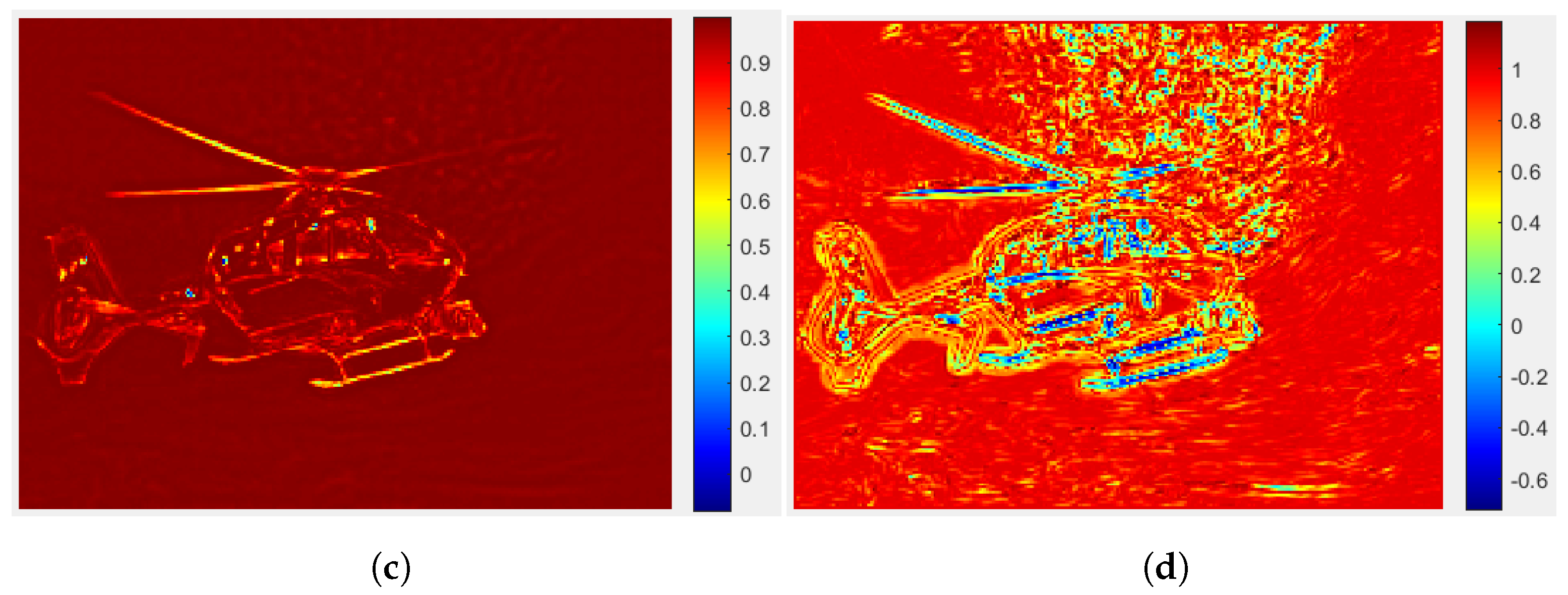
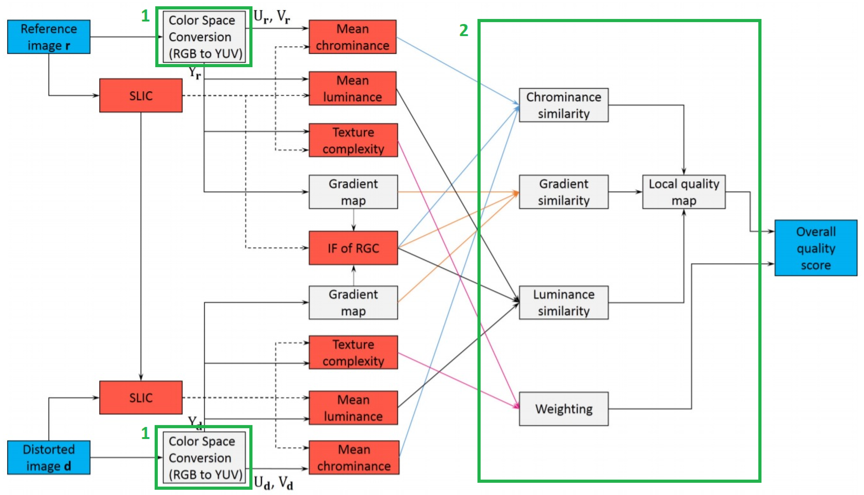
Another proposal to improve image quality assessment using the SPSIM index is to exploit the advantages of the previously described MDSI quality measure. For both SPSIM and MDSI measures, the local similarity of chrominance and image structure is used to determine their values. Both of these components differ for each of the indexes. In the case of the SPSIM index, the chrominance similarity for each of the two channels is calculated separately, whereas for the MDSI index, the chrominance similarity is calculated simultaneously. Similarly, for structural similarity, the MDSI index additionally considers a map of the gradient values for the combined luminance channels, whereas the map of local structural similarities in SPSIM is calculated for each image separately. Therefore, the second proposal for the modification of the SPSIM index consists of determining the the local chrominance and image structure similarity maps based on approaches known from the MDSI index. This approach employs a combination of two methods: SPSIM and MDSI.
Both modifications to the SPSIM algorithm proposed above were separately implemented and compared with other quality measures. The implementation of the new color space was particularly straightforward (two boxes labeled 1 in Figure 4), coming down to simply replacing the transforming formulae from RGB to the proposed color space.
The implementation of the second modification required the use of elements of the MDSI code describing the construction of chrominance and structural similarity maps (box 2 in Figure 4). The implementation details can be found in the paper about MDSI [7]. Furthermore, a solution combining both proposed modifications to SPSIM has also been implemented. In summary, we will consider three modifications of SPSIM: the first one limited to a change of color space and further denoted as SPSIM(YCbCr), the second one operating in YUV color space but using elements of MDSI and denoted as SPSIM (MDSI) and the third one combining the two previous modifications of SPSIM and denoted as (YCbCr_ MDSI). The effectiveness of the resulting modifications to SPSIM is presented in the next section.

4. Experimental Tests

Four benchmark databases (LIVE (2006) [17], TID2008 [18], CSIQ (2010) [19] and TID2013 [20]) were selected for the initial experiment, which are characterized by many reference images, various distortions and different levels of their occurrence in the images.
The LIVE image dataset contains 29 raw images subjected to five types of distortion: JPEG compression, JPEG2000 compression, white noise, Gaussian blur and bit errors occurring during the transmissions of the compressed bit stream. Each type of distortion was assessed by an average of 23 participants. Most images have a resolution of 768 × 512 pixels.
The TID2008 image database contains 1700 distorted images, which were generated using 17 types of distortions, with 4 levels per distortion superimposed on 25 reference images. Subjective ratings were obtained based on 256,428 comparisons made by 838 observers. All images have a resolution of 512 × 384 pixels.
The CSIQ database contains 30 reference images and 866 distorted images using six types of distortion. The distortions used include JPEG compression, JPEG2000 compression, Gaussian noise, contrast reduction and Gaussian blur. Each original image has been subjected to four and five levels of distortions. The average values subjective ratings were calculated on the basis of 5000 ratings obtained from 35 interviewed subjects. The resolution of all images is 512 × 512 pixels.
Image database TID2013 is an extended version of the earlier image collection TID2008. For the same reference images, the number of distortion types has been increased to 24, and the number of distortion levels to 5. The database contains 3000 distorted digital images. The research group, on the basis of which the average subjective ratings of the images were determined, was also increased.
Below is a summary table of the most relevant information about the selected IQA benchmark databases (Table 1). The information on the Konstanz Artificially Distorted Image quality Database (KADID-10k) will be further discussed in Section 5.
The values of the individual IQA measures are usually compared with the values of the subjective ratings for the individual images. Four criteria are used to assess the linearity, monotonicity, and accuracy of such predictions: the Pearson linear correlation coefficient (PLCC), the Spearman rank order correlation coefficient (SROCC), the Kendall rank order correlation coefficient (KROCC) and the root mean squared error (RMSE). The formulae for such comparisons are presented below:
P L C C = i = 1 N ( p i p ¯ ) ( s i s ¯ ) i = 1 N ( p i p ¯ ) 2 ( s i s ¯ ) 2 ,
where p i and s i are raw values of subjective and objective measures, p ¯ and s ¯ are mean values.
S R O C C = 1 6 i = 1 N d i 2 N ( N 2 1 ) ,
where d i means the difference between the ranks of both measures for observation i and N is the number of observations.
K R O C C = N c N d 0.5 ( N 1 ) N ,
where N c and N d are the numbers of concordant and discordant pairs, respectively.
R M S E = 1 N i = 1 N ( p i s i ) 2 ,
where p i and s i are as above.
Table 2, Table 3, Table 4 and Table 5 contain the values of the Pearson, Spearman and Kendall correlation coefficients, and RMSE errors for the tested IQA measures. In each column of the table, the top three results are shown in bold. The two right-hand columns contain the arithmetic average and weighted average values with respect to the number of images in each database. Considering the weighted averages of the calculated correlation coefficients and the RMSE errors, we can see that modifications of the SPSIM index give very good results. A superpixel number of 400 was assumed for the SPSIM index and its three modifications.
The good results obtained for SPSIM and its modifications mainly relate to images from the TID2008 and TID2013 databases. Correlation coefficients computed for CSIQ and LIVE databases are not so clear. The large number of images contained in the TID databases allows reliable transfer of these good results in weighted averages.
The performance of the analyzed new quality measures was measured using a PC with an Intel Core i5-7200U 2.5 GHz processor and 12 GB of RAM. The computational scripts were performed using the Matlab R2019b platform. For each image from the TID2013 set, the computation time of each quality index was measured. The performance of an index was measured as the average time to evaluate the image quality. Table 6 shows average computation times for the chosen IQA measures. SPSIM modifications caused only a few percent increase in the computation time compared to the original SPSIM.

5. Additional Tests on Large-Scale IQA Database

The IQA databases previously used by us contained a limited number of images, most of them using the TID2013 database, i.e., 3000 images. The use of online crowdsourcing for image assessment allowed building larger databases. In recent years, a large-scale image database called KADID-10k (Konstanz Artificially Distorted Image quality Database) [21], which contains more than 10,000 images with subjective scores of their quality (MOS) was created and published. This database contains a limited number of image types (81), a limited number of artificial distortion types (25) and a limited number of levels for each type of distortion (5), resulting in 10,125 digital images. Recently, the KADID-10k database has frequently been used for training, validation and testing of deep learning networks used in image quality assessment [22]. Further use of pretrained convolutional neural networks (CNNs) in IQA algorithms seems promising.
High perceptual quality images from the public website have been rescaled to a resolution 512 × 384 (Figure 5). The artificial distortions used during the creation of the KADID-10k database include blurs, noise, spatial distortions, etc. A novelty was the use of crowdsourcing for subjective IQA in this database. Details of crowdsourcing experiments are described in the article [21].
For SPSIM index tests we used the large-scale IQA database KADID-10k and its modifications with different numbers of superpixels between 100 and 4000. The results obtained are presented in Table 7. The best results for a given number of superpixels are highlighted in bold. In each case, the best results were obtained for the SPSIM modification based on a combination of color space change to YCbCr and application of the similarity maps used in MDSI.
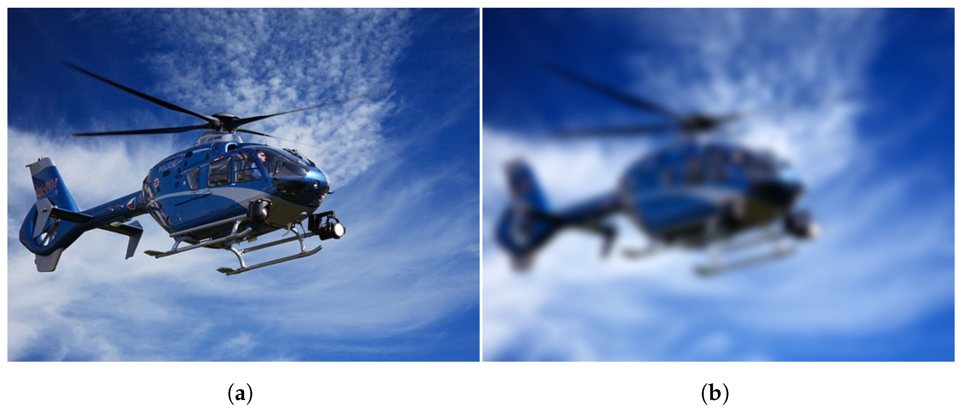
Increasing the number of superpixels improves the values of all four indices. In addition, the effect of the number of superpixels on the computing time for the SPSIM (YCbCr_ MDSI) index was checked for the pair of images presented in Figure 1. Changing the number of superpixels from 100 to 4000 caused a significant increase in the computation time (6.14 times). The choice of the number of superpixels must be a compromise between the computation time and the index values expressing the level of correlation with the MOS scores.

6. Conclusions

The article has shown that there is still much room for improvement in the field of FR-IQA indices. Among the many measures of quality, the SPSIM index using superpixel patches and local similarity maps has recently appeared. In this article, we showed that simple SPSIM modifications (change of color space, different manners of definition of similarity maps inspired by MDSI index) lead to improved correlation with MOS scores. While changing the color space slightly improves these correlations, a different way of defining similarity maps improves them more. The combination of both modifications marked as SPSIM (YCbCr_MDSI) gives the best results. The values achieved by the modified SPSIM quality indices show that there is room for improvement by future research on FR-IQA methods.

Author Contributions

Conceptualization, M.F. and H.P.; methodology, M.F.; software, G.S.; validation, M.F. and H.P.; investigation, M.F. and G.S.; resources, M.F.; data curation, M.F.; writing—original draft preparation, M.F.; writing—review and editing, M.F.; visualization, M.F.; supervision, H.P. All authors have read and agreed to the published version of the manuscript.

Funding

This work was supported by the Polish Ministry for Science and Education under internal grant 02 / 070 / B K 20 / 0005 ( B K - 324 / R A U 4 / 2020 ) for the Department of Data Science and Engineering, Silesian University of Technology, Gliwice, Poland.

Institutional Review Board Statement

Not applicable.

Informed Consent Statement

Not applicable.

Data Availability Statement

Not applicable.

Conflicts of Interest

The authors declare no conflict of interest.

References

  1. Nadenau, M.; Winkler, S.; Alleysson, D.; Kunt, M. Human vision models for perceptually optimized image processing—A review. Proc. IEEE 2000, 32, 1–15. [Google Scholar]
  2. Wang, Z.; Bovik, A.; Sheikh, H.; Simoncelli, E. Image quality assessment: From error visibility to structural similarity. IEEE Trans. Image Process. 2004, 13, 600–612. [Google Scholar] [CrossRef] [PubMed] [Green Version]
  3. Liu, A.; Lin, W.; Narwaria, M. Image quality assessment based on gradient similarity. IEEE Trans. Image Process. 2011, 21, 1500–1512. [Google Scholar] [PubMed]
  4. Zhang, L.; Zhang, L.; Mou, X.; Zhang, D. FSIM: A feature similarity index for image quality assessment. IEEE Trans. Image Process. 2011, 20, 2378–2386. [Google Scholar] [CrossRef] [PubMed] [Green Version]
  5. Xue, W.; Zhang, L.; Mou, X.; Bovik, A.C. Gradient magnitude similarity deviation: A highly efficient perceptual image quality index. IEEE Trans. Image Process. 2013, 23, 684–695. [Google Scholar] [CrossRef] [PubMed] [Green Version]
  6. Zhang, L.; Shen, Y.; Li, H. VSI: A visual saliency-induced index for perceptual image quality assessment. IEEE Trans. Image Process. 2014, 23, 4270–4281. [Google Scholar] [CrossRef] [PubMed] [Green Version]
  7. Nafchi, H.Z.; Shahkolaei, A.; Hedjam, R.; Cheriet, M. Mean deviation similarity index: Efficient and reliable full-reference image quality evaluator. IEEE Access 2016, 4, 5579–5590. [Google Scholar] [CrossRef]
  8. Gu, K.; Li, L.; Lu, H.; Min, X.; Lin, W. A fast reliable image quality predictor by fusing micro- and macro-structures. IEEE Trans. Ind. Electron. 2017, 64, 3903–3912. [Google Scholar] [CrossRef]
  9. Shi, C.; Lin, Y. Full Reference Image Quality Assessment Based on Visual Salience With Color Appearance and Gradient Similarity. IEEE Access 2020, 8, 97310–97320. [Google Scholar] [CrossRef]
  10. Sun, W.; Liao, Q.; Xue, J.H.; Zhou, F. SPSIM: A superpixel-based similarity index for full-reference image quality assessment. IEEE Trans. Image Process. 2018, 27, 4232–4244. [Google Scholar] [CrossRef] [PubMed] [Green Version]
  11. Ren, X.; Malik, J. Learning a classification model for segmentation. In Proceedings of the Ninth IEEE International Conference on Computer Vision, Nice, France, 13–16 October 2013; IEEE: New York, NY, USA, 2003; Volume 1, pp. 10–17. [Google Scholar]
  12. Stutz, D.; Hermans, A.; Leibe, B. Superpixels: An evaluation of the state-of-the-art. Comput. Vis. Image Underst. 2018, 166, 1–27. [Google Scholar] [CrossRef] [Green Version]
  13. Achanta, R.; Shaji, A.; Smith, K.; Lucchi, A.; Fua, P.; Süsstrunk, S. SLIC superpixels compared to state-of-the-art superpixel methods. IEEE Trans. Pattern Anal. Mach. Intell. 2012, 34, 2274–2282. [Google Scholar] [CrossRef] [PubMed] [Green Version]
  14. Mahmoudpour, S.; Schelkens, P. Synthesized view quality assessment using feature matching and superpixel difference. IEEE Signal Process. Lett. 2020, 27, 1650–1654. [Google Scholar] [CrossRef]
  15. Jadhav, M.; Dandawate, Y.; Pisharoty, N. Performance evaluation of structural similarity index metric in different color spaces for HVS based assessment of quality of colour images. Int. J. Eng. Technol. 2013, 5, 1555–1562. [Google Scholar]
  16. ITU-T Recommendation T.871: Information Technology, Digital Compression and Coding of Continuous-Tone Still Images: JPEG File Interchange Format (JFIF); ITU: Geneva, Switzerland, May 2011.
  17. Sheikh, H.; Sabir, M.; Bovik, A. A statistical evaluation of recent full reference image quality assessment algorithms. IEEE Trans. Image Process. 2006, 15, 3440–3451. [Google Scholar] [CrossRef]
  18. Ponomarenko, N.; Lukin, V.; Zelensky, A.; Egiazarian, K.; Carli, M.; Battisti, F. TID2008-a database for evaluation of full-reference visual quality assessment metrics. Adv. Mod. Radioelectron. 2009, 10, 30–45. [Google Scholar]
  19. Larson, E.; Chandler, D. Most apparent distortion: Full-reference image quality assessment and the role of strategy. J. Electron. Imaging 2010, 19, 011006. [Google Scholar]
  20. Ponomarenko, N.; Jin, L.; Ieremeiev, O.; Lukin, V. Image database TID2013: Peculiarities, results and perspectives. Signal Process. Image Commun. 2015, 30, 57–77. [Google Scholar] [CrossRef] [Green Version]
  21. Lin, H.; Hosu, V.; Saupe, D. Kadid-10k: A large-scale artificially distorted iqa database. In Proceedings of the IEEE 2019 Eleventh International Conference on Quality of Multimedia Experience (QoMEX), Berlin, Germany, 5–7 June 2019; pp. 1–3. [Google Scholar]
  22. Varga, D. Composition-preserving deep approach to full-reference image quality assessment. Signal Image Video Process. 2020, 14, 1265–1272. [Google Scholar] [CrossRef]
Figure 1. Similarity maps for the mean deviation similarity index (MDSI): (a) reference image, (b) distorted image, (c) color similarity map C S ^ ( x ) , (d) similarity map G C S ^ ( x ) .
Symmetry 13 00518 g001aSymmetry 13 00518 g001b
Figure 2. Local similarity maps for the superpixel-based similarity (SPSIM) index (100 superpixels): (a) reference image, (b) distorted image, (c) luminance similarity map, (d) chrominance similarity map, (e) gradient similarity map.
Symmetry 13 00518 g002
Figure 3. Local similarity maps for the SPSIM index (400 superpixels): (a) reference image, (b) distorted image, (c) luminance similarity map, (d) chrominance similarity map, (e) gradient similarity map.
Symmetry 13 00518 g003
Figure 4. Flowchart of SPSIM with locations of proposed modifications (green boxes).
Symmetry 13 00518 g004
Figure 5. Konstanz Artificially Distorted Image quality Database (KADID-10k): reference images.
Symmetry 13 00518 g005
Table 1. Comparison of the selected Image Quality Assessment (IQA) databases.
Database NameNo. of Original ImagesNo. of Distortion TypesRatings per ImageEnvironmentNo. of Distorted Images
LIVE29523lab779
TID2008251733lab1700
CSIQ3065~7lab866
TID201325249lab3000
KADID-10k812530crowdsourcing10125
Table 2. Comparison of Pearson Linear Correlation Coefficient (PLCC) values for selected IQA measures.
CSIQLIVETID2008TID2013 PLCC ¯ PLCC w ¯
PSNR0.78570.86820.54050.67880.71830.6796
SSIM0.85790.92120.68030.74590.80130.7651
FSIMc0.91910.96130.87620.87690.90840.8928
GMSD0.95410.96030.87880.85900.91310.8897
VSI0.92790.94820.87620.90000.91310.9033
MDSI0.95310.96590.91600.90850.93590.9236
PSIM0.96420.95840.90770.90800.93460.9218
VCGS0.93010.95090.87760.90000.91470.9044
SPSIM0.93350.95760.89270.90900.92320.9139
SPSIM (YCbCr)0.93460.95640.89460.90990.92380.9148
SPSIM (MDSI)0.93270.95920.90490.91650.92830.9208
SPSIM (YCbCr_MDSI)0.93340.95830.90510.91730.92850.9213
Table 3. Comparison of Spearman Rank Order Correlation Coefficient (SROCC) values for selected IQA measures.
CSIQLIVETID2008TID2013 SROCC ¯ SROCC w ¯
PSNR0.80870.87300.52450.68690.72330.6829
SSIM0.87180.92260.67800.72140.79850.7550
FSIMc0.93090.96450.88400.85100.90760.8847
GMSD0.95700.96030.89070.80440.90310.8675
VSI0.94220.95240.89790.89650.92230.9100
MDSI0.95680.96670.92080.88990.93360.9167
PSIM0.96200.96230.91190.89260.93220.9158
VCGS0.94420.95580.89750.89260.92250.9087
SPSIM0.94340.96070.91040.90430.92970.9182
SPSIM (YCbCr)0.94450.96060.91270.90540.93080.9195
SPSIM (MDSI)0.94250.96300.91310.90520.93100.9195
SPSIM (YCbCr_MDSI)0.94340.96250.91500.90670.93190.9208
Table 4. Comparison of Kendall Rank Order Correlation Coefficient (KROCC) values for selected IQA measures.
CSIQLIVETID2008TID2013 KROCC ¯ KROCC w ¯
PSNR0.59890.68010.36960.49580.53610.4987
SSIM0.67760.74740.48760.52860.61030.5648
FSIMc0.76840.83630.69910.66650.74260.7100
GMSD0.81220.82680.70920.63390.74550.7021
VSI0.78500.80580.71230.71830.75540.7365
MDSI0.81230.83950.75150.71230.77890.7521
PSIM0.82650.82980.73950.71610.77800.7514
VCGS0.78990.81410.71710.71660.75940.7387
SPSIM0.78590.82680.72940.72490.76680.7469
SPSIM (YCbCr)0.78840.82670.73360.72720.76900.7495
SPSIM (MDSI)0.78590.83110.73620.72820.77040.7509
SPSIM (YCbCr_MDSI)0.78770.83070.73930.73060.77210.7530
Table 5. Comparison of RMSE values for selected IQA measures.
CSIQLIVETID2008TID2013 RMSE ¯ RMSE w ¯
PSNR0.162413.55821.12900.91033.94002.4196
SSIM0.134910.63200.98360.82563.14401.9776
FSIMc0.10347.52960.64680.59592.21891.3936
GMSD0.07867.62140.64040.63462.24371.5080
VSI0.09798.68170.64660.54042.49161.4181
MDSI0.07957.07900.53830.51812.05371.4792
PSIM0.06967.79420.56320.51932.23661.2470
VCGS0.09648.45570.64330.54042.43391.3855
SPSIM0.09427.87110.60470.51672.27171.3629
SPSIM (YCbCr)0.09347.97660.59960.51432.29601.3959
SPSIM (MDSI)0.09477.72100.57120.49582.22071.3483
SPSIM (YCbCr_MDSI)0.09427.80480.57050.49352.24071.3573
Table 6. Computation times for algorithms of new quality measures.
IQA Index time ¯ (ms)
MDSI2.14
PSIM5.33
VCGS47.68
SPSIM16.07
SPSIM (YCbCr)16.80
SPSIM (MDSI)15.86
SPSIM (YCbCr_MDSI)17.44
Table 7. The impact of the number of superpixels on SROCC, KROCC, PLCC and Root Mean Squared Error (RMSE) values.
SROCCKROCCPLCCRMSE
No. of SP: 100
SPSIM0.86720.67820.86750.5386
SPSIM (YCbCr)0.86740.67880.86750.5385
SPSIM (MDSI)0.87050.68270.86960.5346
SPSIM (YCbCr_MDSI)0.87090.68360.86980.5342
No. of SP: 200
SPSIM0.87150.68360.87180.5303
SPSIM (YCbCr)0.87190.68430.87190.5301
SPSIM (MDSI)0.87500.68830.87410.5259
SPSIM (YCbCr_MDSI)0.87550.68920.87440.5254
No. of SP: 400
SPSIM0.87430.68710.87440.5254
SPSIM (YCbCr)0.87460.68790.87450.5251
SPSIM (MDSI)0.87770.69170.87660.5209
SPSIM (YCbCr_MDSI)0.87810.69270.87690.5203
No. of SP: 1600
SPSIM0.87550.68970.87490.5242
SPSIM (YCbCr)0.87620.69090.87550.5231
SPSIM (MDSI)0.87910.69450.87740.5193
SPSIM (YCbCr_MDSI)0.87990.69580.87810.5180
No. of SP: 4000
SPSIM0.87590.69080.87510.5239
SPSIM (YCbCr)0.87690.69230.87600.5222
SPSIM (MDSI)0.87970.69590.87780.5186
SPSIM (YCbCr_MDSI)0.88070.69740.87870.5168
Publisher’s Note: MDPI stays neutral with regard to jurisdictional claims in published maps and institutional affiliations.

