SCN: A Novel Shape Classification Algorithm Based on Convolutional Neural Network

Abstract

Shape classification and matching is an important branch of computer vision. It is widely used in image retrieval and target tracking. Shape context method, curvature scale space (CSS) operator and its improvement have been the main algorithms of shape matching and classification. The shape classification network (SCN) algorithm is proposed inspired by LeNet5 basic network structure. Then, the network structure of SCN is introduced and analyzed in detail, and the specific parameters of the network structure are explained. In the experimental part, SCN is used to perform classification tasks on three shape datasets, and the advantages and limitations of our algorithm are analyzed in detail according to the experimental results. SCN performs better than many traditional shape classification algorithms. Accordingly, a practical example is given to show that SCN can save computing resources.

1. Introduction

Shape classification and matching are an important branch of computer vision. In recent years, the research on shape classification is still very popular and has made significant results. It has been widely used in image retrieval, object recognition, text recognition and text retrieval. In the field of computer vision, shapes are generally represented by binary graphs (0 and 1) (as shown in Figure 1). Although this kind of representation method has no basic features such as color and texture, it does not affect people to distinguish their species by relying on the eyes and brain. Studies [1,2,3] show that human eyes are more sensitive to shape and contour features than color and texture features when distinguishing and searching images. Therefore, the shape and contour feature is an advanced feature of more importance than color and texture, which has higher robustness and stability depending on shape recognition and classification.

To let the computer make shape matching and classification is to make a series of matching classification criteria, and then let the computer check and measure whether two or more shapes are similar and belong to the same class according to the established criteria. Traditional shape matching algorithms express the matching degree of two shapes by a numerical value, and the larger the numerical value is, the more similar the two shapes are. Euclidean distance can also be used to express the similarity between shapes, and the larger the distance is, the less similar the two shapes are. Therefore, the general process of shape matching and classification mainly includes the following steps:

• Performing the binary representation of object shapes in the image to obtain shape features;
• Calculating the similarity between two or more shapes according to certain measurement criteria;
• Matching and classifying shapes according to calculation results and premise tasks.

Through studying some methods of shape matching classification [4,5,6,7,8], it was found that the convolutional neural network shows good results in object detection [9]. Therefore, this paper used convolutional neural network for the shape classification task, and good results were achieved. In addition, there are too many network parameters when RGB images are calculated in the convolutional network, so a large amount of computing power will be consumed. Therefore, first converting it to a binary image and then undertaking the convolution operation can save computing power to complete the task of shape retrieval.

The rest of this paper is organized as follows. In Section 2, a review of some well-known methods is presented. Section 3 describes the details of the proposed method. In Section 4, the classification accuracy of shape classification network (SCN) on different shape datasets is compared to other methods. Section 5 gives a practical example. At the end, Section 6 concludes this paper.

2. Related Work

If shape matching and classification want to proceed smoothly, the representation method of shape should be intuitive enough and contain as much information as possible to distinguish them. The description of shape is usually divided into point set, contour and skeleton. The representation methods of the contour and skeleton contain more information than that of the point set. The datasets of this experiment are contour representation, so the traditional contour description methods are mainly introduced.

2.1. Traditional Algorithm

In 2001, shape context proposed by Belongie [4] is a popular shape descriptor based on shape contour features. It describes the distribution of contour sampling points in a log-polar coordinate system with a histogram. Firstly, edge extraction and uniform sampling are carried out to obtain the set of shape points of an object I = {p₁, p₂,…, p_n}. The shape information of each point is represented by the relative vector set formed by all other points and represented by the histogram. The matching cost of point p_i on the target P and point q_i on the target Q is calculated, which is represented by C_i,j:

$$C_{i,j}=C(p_i,q_j)=\frac{1}{2}{\displaystyle \sum _{k=1}^K\frac{{[h_i(k)-h_j(k)]}^2}{h_i(k)+h_j(k)}}$$

(1)

where h_i(k) is the histogram of the shape of the point p_i of the target P; and h_j(k) is the histogram of the shape of point q_i of target Q. The smaller the result is, the more similar they are. However, this descriptor has a poor matching result when there are too many backgrounds and noise points. Daliri [5] combined the shape context description method with strings of symbols to improve the result of shape matching. Ling [6,7] proposed an inner-distance shape context (IDSC) method using the inner distance between contour points, which achieved good results in shape retrieval, but the algorithm complexity was high. Thayananthan [8] combined shape context descriptors with chamfer matching and showed a good performance in object matching in complex scenes.

There is another common method in shape representation: shape representation based on multi-scale theory. This kind of method mainly uses the concave–convex characteristics of plane curves. The concave–convex characteristics of the contour points are obtained by the description method, and then the shape is judged. The curvature scale space (CSS) descriptor proposed by Mokhtarian [9] uses this method. The CSS shape descriptor looks for the curvature zero-crossing of shape contour and takes the combination of extreme point location and scale information as the descriptor. The curvature of each point is calculated as

$$k(u,\sigma )=\frac{\dot{x}(u,\sigma )\ddot{y}(u,\sigma )-\ddot{x}(u,\sigma )\dot{y}(u,\sigma )}{{[\dot{x}{(u,\sigma )}^2+\dot{y}{(u,\sigma )}^2]}^{\raisebox{1ex}{$3$}\!\left/ \!\raisebox{-1ex}{$2$}\right.}}$$

(2)

$$\begin{array}{l}x(u,\sigma )=x(u)\ast g(u,\sigma )\\ y(u,\sigma )=y(u)\ast g(u,\sigma )\end{array}$$

(3)

Among them, $\dot{x}(u,\sigma ),\ddot{x}(u,\sigma ),\dot{y}(u,\sigma ),\ddot{y}(u,\sigma )$ is the first and second derivative of x, y; * is convolution operation; g(u, σ) is a one-dimensional Gaussian function. L(u) = (x(u), y(u)) are the arc length parameters of curve L. The arc length parameter is convolved with g(u,σ) one-dimensional Gaussian function. When the window width σ is increasing, the contour becomes smooth and the zero curvature intersection decreases until the contour becomes convex. CSS descriptors have good robustness to boundary noise. This method is introduced in more detail in [10]. The MCC descriptor proposed by Adamek [11] is similar to CSS. The difference is that MCC measures the concavity of shape by calculating the Euclidean distance between two adjacent scales of a point on the contour, but the computational complexity of this method is higher than CSS. The TAR descriptor proposed by Alajlan [12] describes shapes with triangles composed of contour points. The multi-scale information of shapes is represented by the side lengths of triangles. This descriptor can effectively obtain local and global features. However, the process of feature extraction is complex, the computational complexity is high, and it is sensitive to deformation points. Its robustness is average.

In addition, inner-distance shape context and dynamic programming (IDSC + DP) [13], shape context and dynamic programming (SC + DP) [14], Fourier descriptor (FD) [15] are some classical descriptors. FD [15] is a kind of frequency domain descriptor with high practical value because of its excellent balance between speed and precision. Multiscale distance matrix (MDM) [16] uses a multiscale description method to compute a feature matrix for a shape. Distance interior ratio (DIR) [17] is a relatively new fast descriptor. Angular pattern and binary angular pattern (AP&BAP) [18] is excellent at scale and rotation invariance. More importantly, it is a global shape descriptor. Fourier descriptor based on multiscale centroid contour distance (FMSCCD) [19] is a frequency domain descriptor based on the centroid contour distance (CCD) method, multiscale description, and Fourier transform.

2.2. Development of Deep Learning

In recent years, deep learning has developed rapidly and has shown great ability in object detection and recognition. Therefore, this paper focuses on using convolutional neural network for shape matching and classification tasks. Talking about deep learning, it is necessary to start from the neural network. The neural network is a kind of biomimetic language that can be learned by computers through observation data. Deep learning is a learning technology composed of a group of powerful neural networks. However, until 2006, it was not known how to train neural networks to make them better than traditional methods, except for certain problems. It was not until 2006 when Hinton [20] proposed deep neural network learning technology that deep learning was well developed.

Convolutional neural network adopts a hierarchical structure. The whole system includes a multi-layer network composed of input layer, hidden layers and an output layer (as shown in Figure 2). Only nodes of adjacent layers are connected, while nodes of the same layer and cross-layer are not connected. Each layer can be viewed as a logistic regression model. LeNet5 proposed by Haffner [21] can be regarded as the beginning of a convolutional network, one of the earliest deep convolutional neural networks, and promotes the development of deep learning. Each convolution layer contains three parts: convolution, pooling and nonlinear activation function. Convolution is used to extract the spatial features, and the pooling layer is used to reduce sampling. Sparse connections between layers reduce computational complexity.

In 2012, Alex Krizhevsky [22] proposed the deep convolutional neural network model AlexNet, which can be regarded as a deeper and wider version of LeNet5. AlexNet successfully used ReLU as the activation function of CNN and solved the gradient dispersion problem of Sigmoid function when the network was deep. Meanwhile, in order to prevent overfitting, dropout technology is used to randomly ignore some neurons during training. AlexNet has eight layers requiring training parameters (excluding the pooling layer and LRN layer). The first five layers are convolution layers and the last three layers are full connection layers. See [9] for a specific network structure. In the field of shape classification, Alexnet + VGG 16 + KNN (K-Nearest Neighbor) [23] combined deep features and KNN algorithm to classify leaf-based plant species and achieved a good effect.

3. Method

LeNet5 [21] was first used to recognize handwritten numbers and achieved good results. Considering that the MNIST (Mixed National Institute of Standards and Technology database) [21] dataset is similar to the datasets tested in this paper to a certain extent, handwritten numbers are also equivalent to the shape of an image. So inspired by it, this paper proposes a new algorithm shape classification network (SCN). In addition, many traditional shape description methods are classified according to the characteristics of the shape in a dataset, and this paper wants to propose a more comprehensive shape classification algorithm. Rather than just an algorithm for a specific dataset, it can perform good classification ability under different datasets.

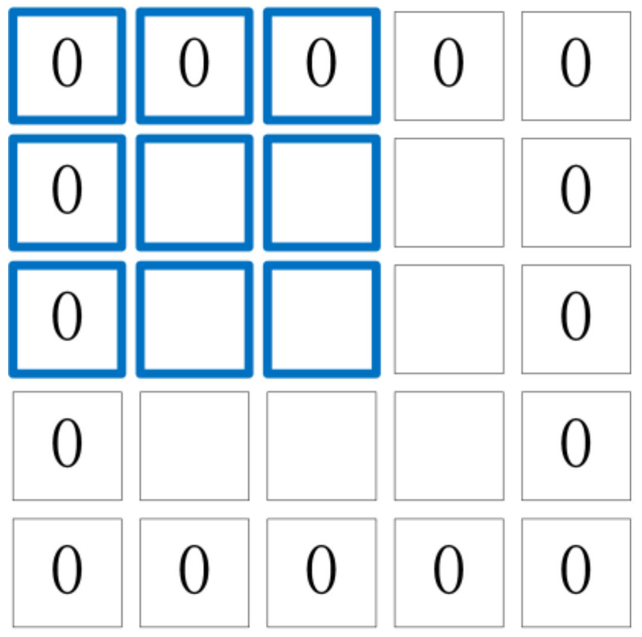
3.1. Size of Convolution Kernel

In the case where the input size of the image is 32 × 32, the general convolution kernel size is 5 × 5, 3 × 3, and 1 × 1 (odd). After the convolution usually requires the padding operation, only if the size of the convolution kernel is odd, the padding can be symmetric from both sides of the image. The datasets used in the experiment is more complex in shape, class, and detail than the handwritten numbers dataset, so the size of the convolution kernel should be determined first. Although the receptive field of 3 × 3 convolution kernel is smaller than that of a large convolution kernel, more local information can be extracted. Other unnecessary and influential information is extracted at the same time, but this effect can be avoided by using a pooling layer. Therefore, it is more suitable for complex shapes. Of course, the convolution kernel is not as small as possible, especially for sparse data (Figure 3). When using a relatively small convolution kernel (such as a 1 × 1 convolution kernel), the receptive field is too small to extract many useful features. In this paper, the convolution kernel size of the first two layers is 3 × 3 to extract local features better. The size of the convolution kernel of the last convolutional layer is 5 × 5, and it is more inclined to extract global features, which can better adapt to complex datasets.

The simple image information means that the boundary of the image does not contain much meaningful information. However, some shapes extend to the edges of the image. In order to ensure that the edge information of the image can be calculated multiple times, padding is added to the image. If the padding is not added, the edge of the input image information will only be computed once, and the pixels in the middle of the image will be traversed many times. Thus, the reference level of the boundary information will be reduced. However, after adding the padding, the new boundary is computed during actual processing (as shown in Figure 4).

3.2. Fine-Tuning

The main idea of fine-tuning is to use the weight information of the original model as the initialization parameter of the new model to be trained. Because the current various models that use deep learning to classify images have too little correlation between their characteristics with shapes, and we expanded the dataset to tens of thousands, which is enough for the network to retrain without pre-training and fine-tuning. At the same time, we used MNIST [21] and CIFAR-10 [24] models to fine-tune and then experiment, though the results were not good. In our opinion, the correlation between the MNIST [21] dataset with the shape dataset we used is higher than the others. If this result is not good, the other performance will be worse. Theoretically, it will actively and quickly enter a poor local optimal point. The global optimal point will not be approached step by step, so that the entire network performance cannot achieve good results. Therefore, fine-tuning is not used in this experiment.

3.3. Addition of BN Layer

The batch normalization (BN) [25] layer is just like the activation function layer, convolution layer, full connection layer, pooling layer, etc. It also belongs to the network layer. In addition to the output layer, the other layers are constantly updated with the training as the low-level network is trained. As long as the first few layers of the network change slightly, the next few layers are cumulatively enlarged. Once the distribution of input data at a certain layer of the network changes, then this layer of network needs to adapt to learn this new data distribution. Thus, if the distribution of training data has been changing during the training process, it will affect the training speed of the network. Therefore, when inputting each layer, adding a pre-processing operation before input is very beneficial to the whole training process. The proposal of BN is to solve the situation in which the distribution of data in the middle layer changes during the training process.

For the neural network input data preprocessing, the effective algorithm is whitening preprocessing. However, the whitening calculation is too large, and the whitening is not differentiable everywhere. Thus, in deep learning, the calculation cost of using whitening is too large to be used rarely. After whitening pretreatment, the data meets the conditions: (1) the correlation between features is reduced, which is equivalent to principal component analysis (PCA); (2) data mean and standard deviation normalization, that is, the mean value of each dimension is 0, the standard deviation is 1. If the dimension of the data feature is relatively large, it is necessary to use the PCA algorithm to reduce the dimension, that is, to achieve the first requirement of whitening. It is necessary to calculate the feature vector, and the calculation amount is very large. Therefore, in order to simplify the calculation, the BN algorithm ignores the first requirement. For pre-processing, the following formula should be used, that is, to approximate the whitening pretreatment:

$${\widehat{x}}^{(k)}=\frac{x^{(k)}-E[x^{(k)}]}{\sqrt{Var[x^{(k)}]}}$$

(4)

Using this formula, the input data of a layer of network will be normalized. However, in order to prevent the use of normalization processing to affect the distribution of features learned in the previous layer, the BN algorithm is transformed and reconstructed, and learnable parameters $\gamma ,\beta$ are introduced:

$$y^{(k)}={\gamma }^{(k)}{\widehat{x}}^{(k)}+{\beta }^{(k)}$$

(5)

Each neuron will have a pair of such parameters $\gamma ,\beta$. Thus, when the parameters are met:

$$\begin{array}{l}{\gamma }^{(k)}=\sqrt{Var[x^{(k)}]}\\ {\beta }^{(k)}=E[x^{(k)}]\end{array}$$

(6)

It is possible to recover the distribution of features learned in the previous layer and eliminate the effects.

Therefore, the BN algorithm introduces the learning parameters $\gamma ,\beta$, which allows the network to learn to recover the distribution of the original network. It not only preprocesses the data well, but also improves the generalization ability of the network. The entire algorithm flow of the forward conduction of the Batch Normalization network layer is:

• Input data x₁…x_m over a mini-batch B = {x_1…m} sequentially, which are the data ready to enter the activation function;
• Find the data average by ${\mu }_B=\frac{1}{m}{\displaystyle \sum _{i=1}^m{x}_i}$;
• Using the formula ${\sigma }_B^2=\frac{1}{m}{\displaystyle \sum _{i=1}^m{(x_i-{\mu }_B)}^2}$ to obtain the variance of the input data;
• The data ire normalized by ${\widehat{x}}_i=\frac{x_i-{\mu }_B}{\sqrt{{\sigma }_B^2+\theta }}$, or referred to as normalization;
• The parameters $\gamma ,\beta$ are trained by the formula $y_i=\gamma {\widehat{x}}_i+\beta \equiv B{N}_{\gamma ,\beta }(x_i)$, and the output y value is obtained by linear transformation of $\gamma ,\beta$.

Therefore, it is concluded that in the case of forward propagation, by learning the reconstruction parameters $\gamma ,\beta$, learning to recover the feature distribution that the original network has to learn, has a positive impact on the training process. In the case of backpropagation, $\gamma ,\beta$ and associated weights are obtained by chain derivation.

The reason for placing the BN layer behind the convolutional layer is explained in the BN paper [25]. Take the second layer of the network as an example: the input of the second layer is calculated by the parameters of the first layer and input, while the parameters of the first layer are always changing during the whole training process, so it will inevitably cause changes in the distribution of input data of each subsequent layer. We call the change of data distribution in the middle layer of the network during the training process as “Internal Covariate Shift”. Thus, the Internal Covariate Shift problem can be solved by performing a BN operation before the data goes to the next layer.

The output distribution of the nonlinear element will change during the training process. Normalization cannot eliminate its variance offset. On the contrary, the output of full connection and convolution layers is generally a symmetric, non-sparse distribution, more like a Gaussian distribution, and normalization produces a more stable distribution. Because we did not perform pre-training and fine-tuning with the existing model, the entire network was retrained, and the test set and the training set have completely different shapes, i.e., the test set and the training set have different distributions. The essence of the neural network learning process is to learn the data distribution. Once the distribution of the training data and the test data are different, the generalization ability of the network is greatly reduced. On the other hand, once the distribution of each batch of training data is different, the network must learn to adapt to different distributions in each iteration, which will greatly reduce the training speed of the network. This is why we use the BN layer to perform a normalized preprocessing on the data.

Therefore, after using the BN algorithm in the SCN network structure, it not only allows the use of a larger learning rate, which greatly improves the speed of training, but also normalizes the parameters to improve the network generalization ability. It has a positive effect on shape classification tasks.

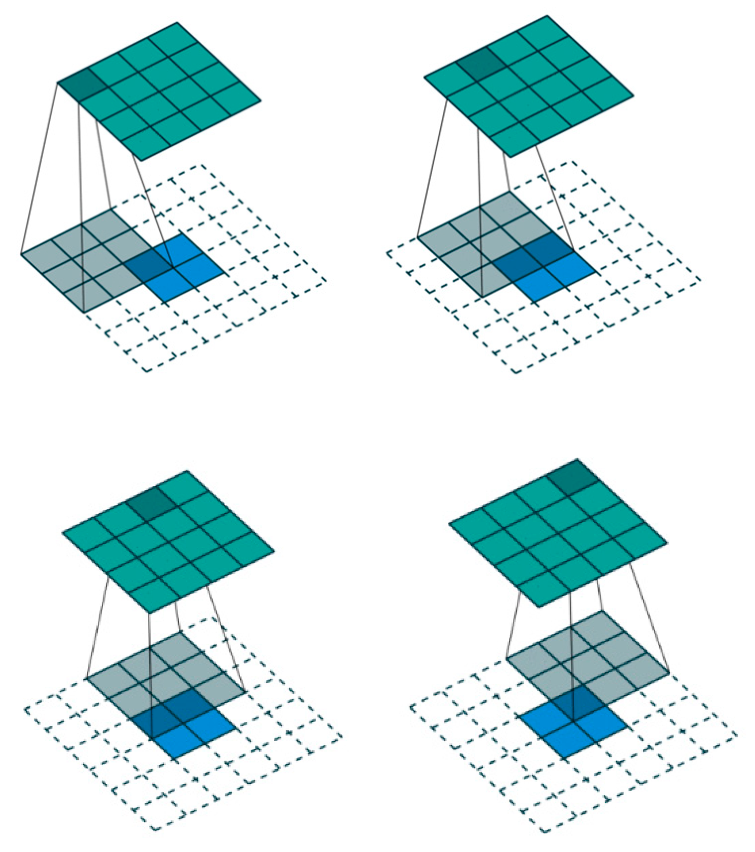
3.4. Application of the Transposed Convolution Layer

When transposed convolution was first proposed as deconvolution [26], the deconvolution here is only conceptually opposite to the traditional convolution. The traditional convolution is to generate a feature map from the image, and the deconvolution is to find a set of kernel and feature maps with the unsupervised method and let them reconstruct the image. The feature map obtained by the convolution in CNN was restored to the pixel space by deconvolution to observe which pattern images were sensitive to the specific feature map. The deconvolution is not the reversible operation of convolution, but the transposed convolution, so it is always called transposed convolution in deep learning field. The general transposed convolution operation is visualized as shown in Figure 5 [27].

In 2014, Jonathan Long [28] used up-sampling in the full convolutional network (FCN) to achieve good results for semantic segmentation. There are some similarities between object contour and image semantic segmentation (image semantic segmentation can also be regarded as the extraction of shape contour), so this paper adds a layer of operation similar to up-sampling in the network structure, that is, adding a transposed convolution layer. The transposed convolution layer is used to up-sample the feature map of the last convolutional layer to restore or enlarge its image size, so that a prediction can be generated for each pixel while preserving the spatial information in the original input image. Finally, the feature images with up-sampling are classified. That is, the classification from the image level is further extended to the classification at the pixel level.

The learning of the transposed convolution is an alternative optimization, which first optimizes the feature map z and then optimizes the convolution kernel f. If there is a multi-layer transposed convolution operation, it is also layer-by-layer training. The first step is to learn the feature map. It is difficult to directly learn the loss function of the transposed convolution layer. The reason is that the points at different positions in the feature map are heavily coupled because of the convolution kernel. Therefore, selecting a proxy variable x, making z approach x, then regularizing x, and alternately optimizing z and x:

$$\begin{array}{l}{\widehat{C}}_l(y)=\frac{\lambda }{2}{\displaystyle \sum _{i=1}^I{\displaystyle \sum _{c=1}^{K_{l-1}}\parallel {\displaystyle \sum _{k=1}^{K_l}{g}_{k,c}^l(z_{k,l}^i\oplus }}}{f}_{k,c}^l)-z_{c,l-1}^i{\parallel }_2^2\\ +\frac{\beta }{2}{\displaystyle \sum _{i=1}^I{\displaystyle \sum _{k=1}^{K_l}\parallel z_{k,l}^i-x_{k,l}^i}}{\parallel }_2^2+{\displaystyle \sum _{i=1}^I{{\displaystyle \sum _{k=1}^{K_l}\left|x_{k,l}^i\right|}}^p}\end{array}$$

(7)

The second step is to learn the convolution kernel f, which can be completed by a normal gradient descent. The specific algorithm flow is shown in [29].

3.4.1. Transposed Convolution

In [29], it was mentioned that in the past learning method, the original pixel of the image is lost when learning layer by layer, and the target of learning is only the feature map of the upper layer. Thus, the connection relationship between the high-level filter and the input image is not so strong, leading to a learning effect which is not good. Therefore, this paper uses transposed convolution.

Inspired by DCGAN (Deep Convolution Generative Adversarial Networks) [30], the GAN (Generative Adversarial Networks) network required generative models and generated images from the input data of specific distribution through transposed convolution. As shown in Figure 6, a 4 × 4 shape binary image shown Figure 6a is convolved with a 3 × 3 convolution kernel shown in Figure 6b to obtain a 2 × 2 feature image seen in Figure 6c. Then, transposed convolution is performed on the obtained feature image Figure 6c. First, 0 is added to the feature image to obtain a size that can be convolved to obtain the image Figure 6d, and then convolution calculation is performed with a 3 × 3 convolution kernel shown in Figure 6e,f, which is the feature image obtained after transposed convolution. From Figure 6f and Formula (8), it can be inferred that the transposed convolution increases the horizontal and vertical gradients between pixels. Therefore, when the transposed convolution layer is added, the experimental accuracy rate will be improved:

$$\begin{array}{l}dx(i,j)=\frac{I(i+1,j)-I(i-1,j)}{2}\\ dy(i,j)=\frac{I(i,j+1)-I(i,j-1)}{2}\end{array}$$

(8)

3.4.2. Checkerboard Effect

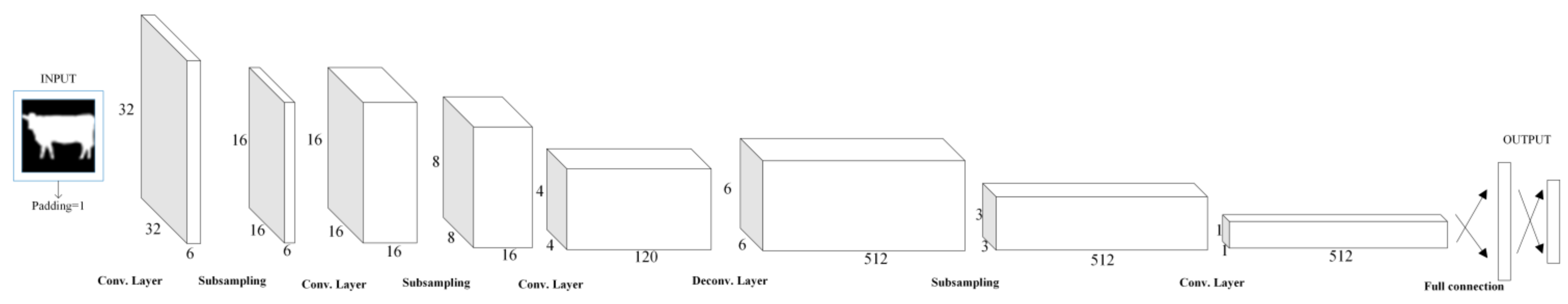
The transposed convolution operation is a method of up-sampling operation that allows the model to draw a block on a high-resolution image through each point. This is related to the stride and kernel size of the transposed convolution. If the stride and kernel size are not properly selected, the checkerboard effect is easy to occur, which has an adverse effect on the experimental results. For example, in Figure 7, the upper black grid represents a certain pixel in the original image, and the white represents the stride in the transposed convolution, which is generally filled with 0. The next layer is the image generated by transposed convolution. When stride cannot divide the kernel size, the checkerboard effect will appear. Although it can be weakened to a certain extent when it is divisible, it cannot be completely eliminated. Therefore, in this experiment, the choice of divisibility not only reduces the influence of the checkerboard effect, but also improves the learning ability of the entire network.

3.5. Architecture

The size of the convolution kernel of the first two convolutional layers is 3 × 3, with stride 1 and padding 1. The convolutional kernel of the third convolutional layer is 5 × 5. The number of transposed convolution output channels is 512, the kernel size is 3 × 3, and the stride is 1. The final convolutional kernel is 3 × 3 and outputs 512 channels. Max-pooling is performed over a 2 × 2 pixel window, with stride 2. The last full connection layer is based on the number of classifications. Some detailed parameters and the schematic diagram of the entire network architecture is shown in Figure 8.

4. Experiment

This experiment uses a GTX 1050Ti GPU for training and testing under Linux. Three datasets were used in this experiment: Animals [31], MPEG(Moving Picture Experts Group)-7 CE-1 Part B [32] and Swedish Plant Leaf [33]. The total amount of data in each dataset is still not enough. When the dataset is too small and the data sample is insufficient, deep learning has no obvious advantage over other traditional algorithms. Therefore, we take a data augmentation on the original dataset to ensure the effective training of the model. Each image is rotated 10° counterclockwise in turn, 36 times in total (as shown in Figure 9), and the dataset is expanded to 36 times of the original. It cannot only improve the robustness of the model, but also improves the generalization ability of the model. The algorithm SCN proposed in this paper is compared with several traditional shape algorithms on three different datasets, with the classification accuracy as the discriminant standard.

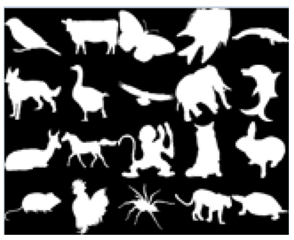
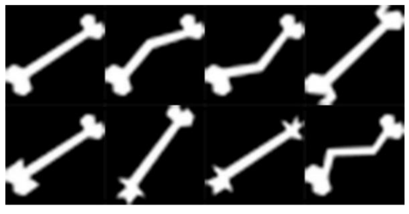
4.1. Performance on Animals Dataset

The Animals [31] dataset has 20 classes (as shown in Figure 10), and each class has 100 similar shapes (part of the shape is shown in Figure 11). After a data augmentation, the new dataset has 72,000 images. There are 3600 images in each class, 2520 of which are selected as the training set and the remaining 1080 as the test set, so that the number of training set and test set is roughly divided into 7:3.

Compared with many traditional algorithms, the classification accuracy of our algorithm SCN is higher. The main idea of the traditional shape classification algorithm is to classify based on the proposed descriptor, but the various shapes included in the Animals dataset range from simple to complex, with varying degrees of complexity. Therefore, traditional algorithms have limitations on such a complex dataset, and SCN has good performance (as shown in

Table 1. Performance of the different algorithms on Animals dataset.

Method	Classification Accuracy
FMSCCD [19]	37.33%
IDSC-WFW (a weighted Fourier and wavelet-like descriptor based on inner distance shape context) [34]	49.36%
DIR [17]	46.45%
AP & BAP [18]	52.79%
MDM [16]	35.81%
FPD (farthest point distance) [35]	26.63%
FD [15]	27.97%
FASD & FMSCCD (fast angle scale descriptor and FMSCCD) [19]	37.85%
FD-ASD (Fourier descriptor-angle scale descriptor) [36]	27.44%
ASD & CCD (angle scale descriptor and centroid contour distance) [36]	39.30%
SC + DP [14]	67.27%
IDSC + DP [13]	70.99%
HSC (Hierarchical string cuts) [37]	56.80%
SCN (ours)	75.39%

).

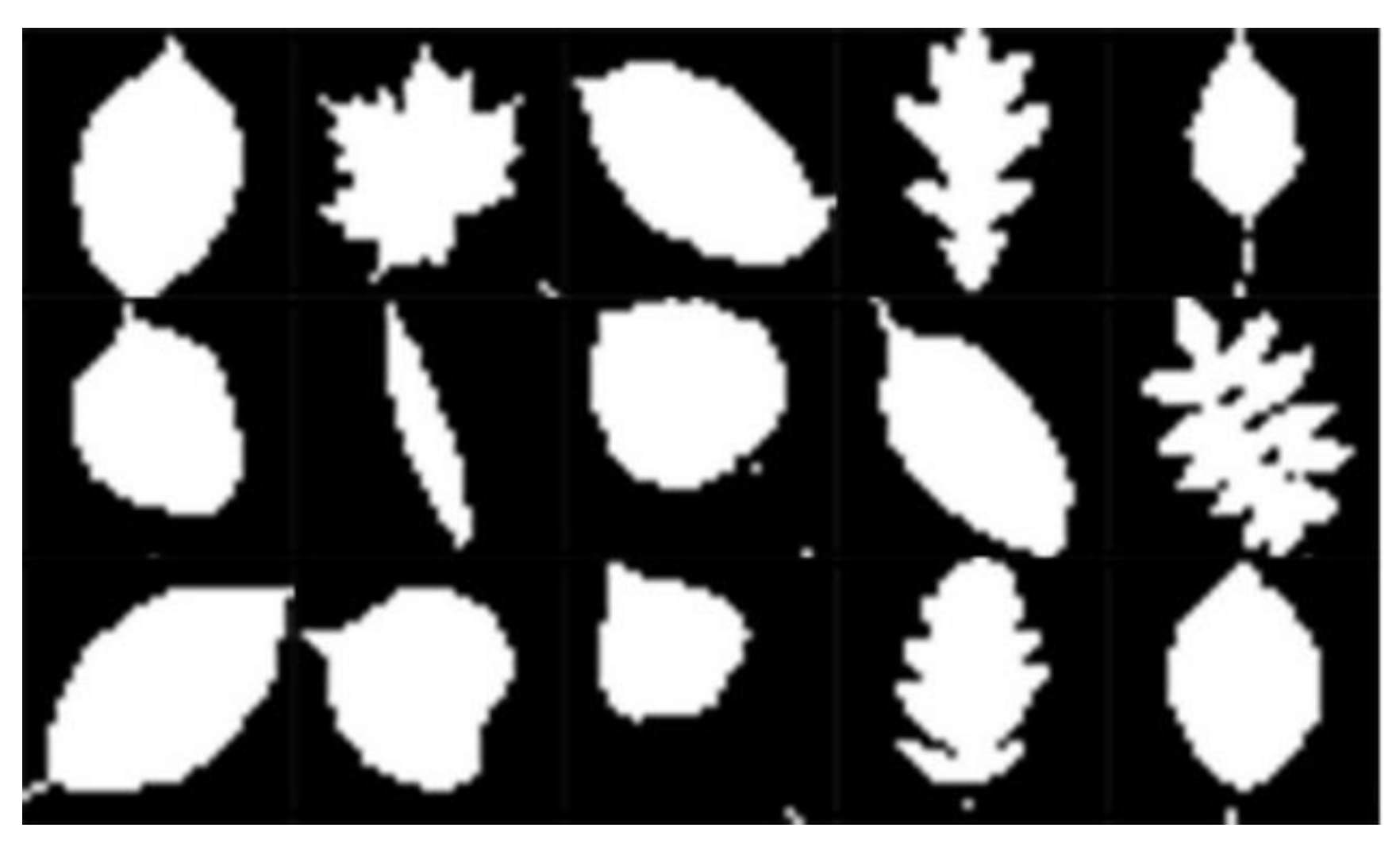
4.2. Performance on Swedish Plant Leaf Dataset

The Swedish Plant Leaf [33] dataset has 15 classes (as shown in Figure 12), and each class has 75 similar shapes (part of the shape is shown in Figure 13), performing the same operations and requirements as the previous two datasets. The new dataset consists of 40,500 images, with 2700 for each class, 1908 for the training set and 792 for the test set.

Swedish Plant Leaf dataset has a few classes and the samples are not very complex and have obvious features. After data augmentation, the number of samples for each class of data is sufficient for training and testing. Both the traditional algorithm and the SCN have good performance, while the SCN can extract the details better, so the classification accuracy of the SCN is higher than the traditional algorithm (as shown in

Table 2. Performance of different algorithms on Swedish Plant Leaf dataset.

Method	Classification Accuracy
FMSCCD [19]	87.98%
IDSC-WFW [34]	93.66%
DIR [17]	88.20%
MDM [16]	87.32%
FPD [35]	77.16%
FD [15]	82.40%
FASD & FMSCCD [19]	91.04%
FDASD [36]	87.32%
ASD & CCD [36]	85.14%
MLBP (modified LBP) [38]	96.83%
SCN (ours)	94.46%

).

4.3. Performance on MPEG-7 CE-1 Part B DATASET

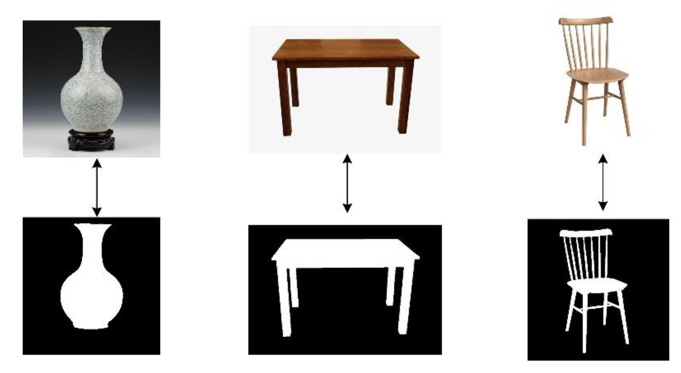
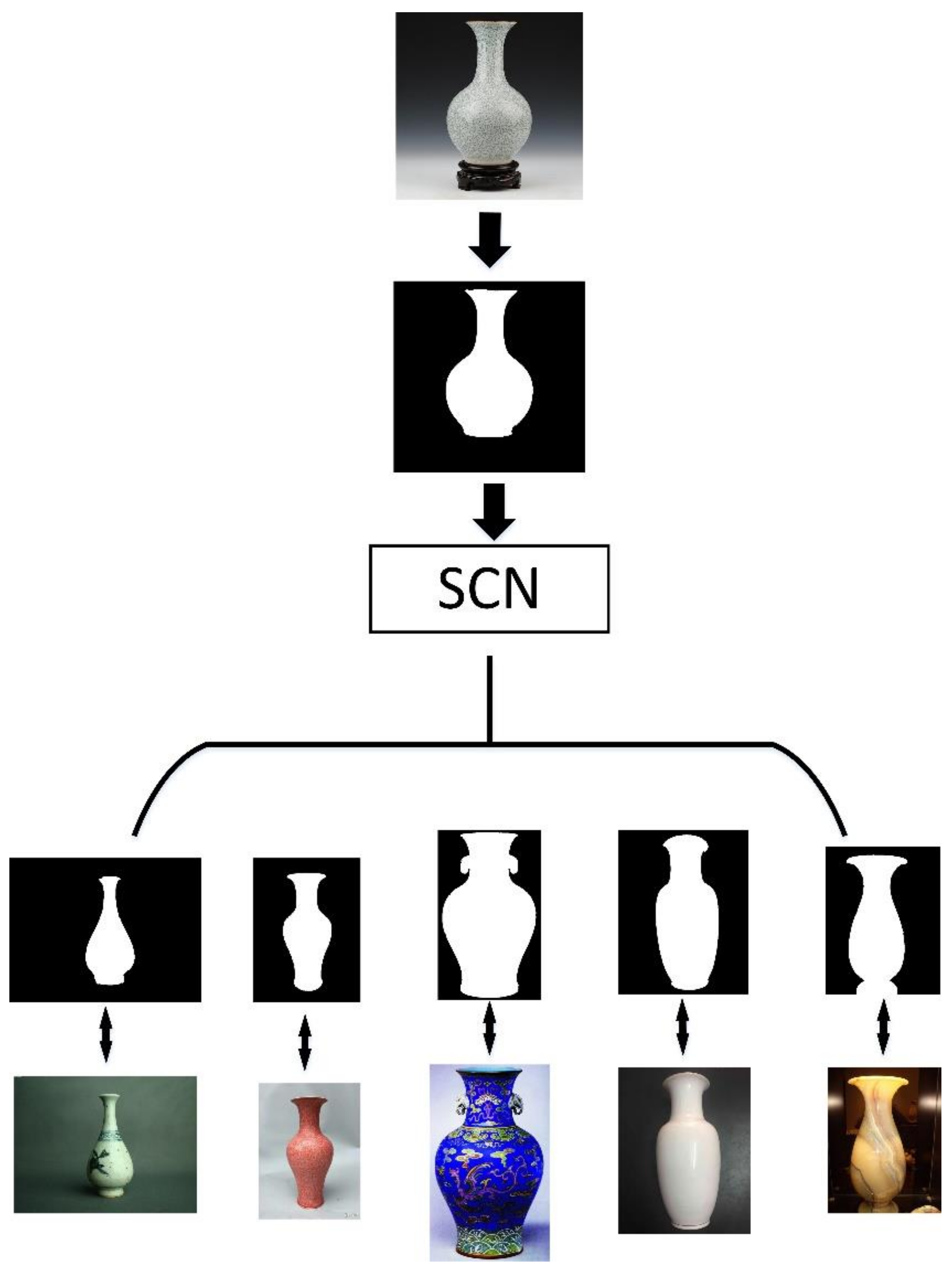
The MPEG-7 CE-1 Part B [32] dataset has 70 classes (we only show 20 of them in Figure 14), and each class has 20 similar shapes (part of the shapes is shown in Figure 15). After data augmentation, the MPEG-7 dataset has 50,400 images. Similarly, the training set and test set were divided into 7:3. There were 720 images in each class, 504 of which were selected as the training set and the remaining 216 as the test set.

Although the classes of the MPEG-7 dataset are diverse, the similarity between different classes is relatively small, and each shape has obvious features, which makes it easy to distinguish. Therefore, the classification accuracy of the traditional algorithms is generally higher. Although the performance of SCN is better than them, the training samples of each class are less than the other two datasets, so the accuracy is improved less (as shown in

Table 3. Performance of the different algorithms on the MPEG-7 dataset.

Method	Classification Accuracy
FASD & FMSCCD [19]	88.57%
DIR [17]	87.62%
MDM [16]	88.33%
FPD [35]	77.86%
FD [15]	77.86%
FMSCCD [19]	77.62%
FDASD [36]	85.24%
ASD & CCD [36]	89.76%
SCN (ours)	90.99%

).

Precision, Recall and F1-score are respectively shown in

Table 4. Precision, recall and F1-score on different datasets.

Dataset	Precision	Recall	F1-Score
Animals [31]	77.21%	74.39%	76.77%
Swedish Plant Leaf [33]	93.38%	92.47%	93.16%
MPEG-7 CE-1 Part B [32]	83.23%	86.41%	85.79%

. In these three datasets (Animals [31], MPEG-7 CE-1 Part B [32] and Swedish Plant Leaf [33]), the number of similar shapes in each class of Animals was the largest, each class having 100 similar shapes, and the least was MPEG-7 CE-1 Part B, where each class only had 20 similar shapes. When the similar shapes were sufficient, it has a positive effect on the learning ability of the network, and the SCN’s accuracy is also better than traditional algorithms. However, on the other two datasets, as the number of similar shapes decreases, the learning ability and performance of SCN will gradually reach the limit. Compared with the traditional algorithm, although it has improved, it is not significant. Therefore, the ability of SCN is related to the number of similar shapes in the same class. The greater the number of similar shapes, the better the performance of SCN. To facilitate further research, the trained model and model code are made publicly available on https://github.com/Zzz-zcy/SCN (accessed on 10 March 2021).

5. Application

The SCN algorithm can be used in the shape retrieval field of cultural heritage [39,40]. We included a description of the possible application scenarios in order to make it easier to understand. A practical example was given below so that it can be useful better to understand the operation of the entire proposed system, from beginning to end. Taking the shape of a vase as an example, we randomly selected 50 pictures. Most of them were vases, with a few pictures of tables, chairs and other objects.

Firstly, all images are preprocessed to get adaptive binarization after saliency detection, and each binary image has a special label corresponding to the original image (as shown in Figure 16). Then, input the shape of a vase into the algorithm, and some binary shape images similar to the shape of the input image can be obtained. Due to the special label correspondence, the images that are all vases are finally retrieved. The entire flow chart is shown in Figure 17. Because there are too many network parameters when RGB images are calculated in the convolutional network, a large amount of computing power will be consumed. Therefore, converting it to a binary image first and then convolution operation can save computing power to complete the task of shape retrieval.

6. Conclusions

In this paper, a new shape classification algorithm SCN is proposed. Compared with the traditional shape classification method using descriptors, our algorithm can classify different shape datasets more comprehensively. For example, the MDM [17] algorithm is a classification algorithm proposed for the shape of plant leaves. The classification accuracy of plant leaves shapes is good, but when MDM [17] is applied to other datasets, such as Animals [31], which have both simple shape structure and complex shape structure, the results will not be so ideal.

Moreover, this algorithm can also be used in the field of remote sensing images in the future, because objects in remote sensing images are more blurred than ordinary scene images, so it is difficult to classify them with texture and point features. Without texture features and feature points, people can only use shape features to classify objects. The algorithm SCN in this paper performs good classification accuracy in three shape datasets (Animals [31], MPEG-7 CE-1 Part B [32] and Swedish Plant Leaf [33]) with different complex conditions, indicating that the algorithm SCN is more comprehensive than other traditional algorithms and will be helpful for future practical applications.

References

1. Mouine, S.; Yahiaoui, I.; Verroust-Blondet, A.V. A shape-based approach for leaf classification using multiscale triangular representation. In Proceedings of the 3rd ACM Conference on Multimedia Retrieval, Dallas, TX, USA, 16–19 April 2003; pp. 127–134. [Google Scholar]
2. Milios, E.; Petrakis, E. Shape retrieval based on dynamic programming. IEEE Trans. Image Process. 2000, 9, 141–147. [Google Scholar] [CrossRef] [PubMed] [Green Version]
3. Zheng, Y.; Guo, B.; Yan, Y.; He, W. O2O Method for Fast 2D Shape Retrieval. IEEE Trans. Image Process. 2019, 28, 5366–5378. [Google Scholar] [CrossRef]
4. Zahn, C.T.; Roskies, R.Z. Fourier descriptors for plane closed curves. IEEE Trans. Comput. 1972, 100, 269–281. [Google Scholar] [CrossRef]
5. Daliri, M.R.; Torre, V. Robust symbolic representation for shape recognition and retrieval. Pattern Recognit. 2008, 41, 1782–1798. [Google Scholar] [CrossRef]
6. Ling, H.B.; Jacobs, D.W. Using the inner-distance for classification of articulated shapes. In Proceedings of the 2005 IEEE Conference on Computer Vision and Pattern Recognition (CVPR), San Diego, CA, USA, 20–26 June 2005; IEEE: Washington, DC, USA, 2005; pp. 719–726. [Google Scholar]
7. Wang, B.; Gao, Y.; Sun, C.; Blumenstein, M.; La Salle, J. Can walking and measuring along chord bunches better describe leaf shapes? In Proceedings of the IEEE Conference on Computer Vision and Pattern Recognition, Honolulu, HI, USA, 21–26 July 2017; pp. 6119–6128. [Google Scholar]
8. Thayananthan, A.; Stenger, B.; Torr, P.H.S.; Cipolla, R. Shape context and chamfer matching in cluttered scenes. In Proceedings of the 2003 IEEE Computer Society Conference on Computer Vision and Pattern Recognition (CVPR), Madison, WI, USA, 16–22 June 2003; IEEE: Washington, DC, USA, 2003; pp. 127–133. [Google Scholar]
9. Mokhtarian, F.; Abbasi, S.; Kittler, J. Efficient and robust retrieval by shape content through curvature scale space. In Proceedings of the International Workshop on Image Databases and Multi-Media Search, Amsterdam, The Netherlands, 22–23 August 1996; pp. 35–42. [Google Scholar]
10. Mokhtarian, F.; Bober, M. Curvature Scale Space Representation: Theory, Applications, and MPEG-7 Standardization; Kluwer Academic Publishers: Dordrecht, The Netherlands, 2003. [Google Scholar]
11. Adamek, T.; O’Connor, N.E. A multiscale representation method for nonrigid shapes with a single closed contour. IEEE Trans. Circuits Syst. Video Technol. 2004, 14, 742–753. [Google Scholar] [CrossRef] [Green Version]
12. Alajlan, N.; El Rube, I.; Kamel, M.S.; Freeman, G. Shape retrieval using triangle-area representation and dynamic space warping. Pattern Recognit. 2007, 40, 1911–1920. [Google Scholar] [CrossRef]
13. Ling, H.; Jacobs, D.W. Shape classification using the inner-distance. IEEE Trans. Pattern Anal. Mach. Intell. 2007, 29, 286–299. [Google Scholar] [CrossRef] [PubMed]
14. Belongie, S.; Malik, J.; Puzicha, J. Shape matching and object recognition using shape contexts. IEEE Trans. Pattern Anal. Mach. Intell. 2002, 24, 509–522. [Google Scholar] [CrossRef] [Green Version]
15. Zhang, D.; Lu, G. Study and evaluation of different Fourier methods for image retrieval. Image Vis. Comput. 2005, 23, 33–49. [Google Scholar] [CrossRef]
16. Hu, R.X.; Jia, W.; Ling, H.; Huang, D. Multiscale distance matrix for fast plant leaf recognition. IEEE Trans. Image Process. 2012, 21, 4667–4672. [Google Scholar] [PubMed]
17. Kaothanthong, N.; Chun, J.; Tokuyama, T. Distance interior ratio: A new shape signature for 2D shape retrieval. Pattern Recognit. Lett. 2016, 78, 14–21. [Google Scholar] [CrossRef] [Green Version]
18. Hu, R.-X.; Jia, W.; Ling, H.; Zhao, Y.; Gui, J. Angular pattern and binary angular pattern for shape retrieval. IEEE Trans. Image Process. 2014. 23, 1118–1127.
19. Zheng, Y.; Guo, B.; Chen, Z.; Li, C. A Fourier Descriptor of 2D Shapes Based on Multiscale Centroid Contour Distances Used in Object Recognition in Remote Sensing Images. Sensors 2019, 19, 486. [Google Scholar] [CrossRef] [Green Version]
20. Hinton, G.E.; Salakhutdinov, R.R. Reducing the Dimensionality of Data with Neural Networks. Neural Comput. 2006, 18, 1527. [Google Scholar] [CrossRef]
21. LeCun, Y.; Bottou, L.; Bengio, Y.; Haffner, P. Gradient-based learning applied to document recognition. Proc. IEEE 1998, 86, 2278–2324. [Google Scholar] [CrossRef] [Green Version]
22. Krizhevsky, A.; Sutskever, I.; Hinton, G.E. ImageNet classification with deep convolutional neural networks. In Proceedings of the International Conference on Neural Information Processing Systems; Curran Associates Inc.:: Red Hook, NY, USA, 2012. [Google Scholar]
23. Türkoğlu, M.; Hanbay, D. Combination of Deep Features and KNN Algorithm for Classification of Leaf-Based Plant Species. In Proceedings of the 2019 International Artificial Intelligence and Data Processing Symposium (IDAP), Malatya, Turkey, 21–22 September 2019; pp. 1–5. [Google Scholar] [CrossRef]
24. Krizhevsky, A. Learning Multiple Layers of Features from Tiny Images. Master’s Thesis, Department of Computer Science, University of Toronto, Toronto, ON, Canada, 2009. [Google Scholar]
25. Ioffe, S.; Szegedy, C. Batch Normalization: Accelerating Deep Network Training by Reducing Internal Covariate Shift. In Proceedings of the International Conference on Machine Learning, Lille, France, 6–11 July 2015. [Google Scholar]
26. Zeiler, M.D.; Krishnan, D.; Taylor, G.W.; Fergus, R. Deconvolutional networks. In Proceedings of the 2010 IEEE Computer Society Conference on Computer Vision and Pattern Recognition, San Francisco, CA, USA, 13–18 June 2010. [Google Scholar]
27. Vdumoulin.Conv_Arithmetic. Available online: https://github.com/vdumoulin/conv_arithmetic (accessed on 15 December 2020).
28. Long, J.; Shelhamer, E.; Darrell, T. Fully Convolutional Networks for Semantic Segmentation. arXiv 2015, arXiv:1411.4038. [Google Scholar]
29. Zeiler, M.D.; Taylor, G.W.; Fergus, R. Adaptive deconvolutional networks for mid and high level featurelearning. In Proceedings of the 2011 International Conference on Computer Vision, Barcelona, Spain, 6–13 November 2011. [Google Scholar]
30. Radford, A.; Metz, L.; Chintala, S. Unsupervised representation learning with deep convolutional generative adversarial networks. In Proceedings of the 4th International Conference on Learning Representations, ICLR 2016—Conference Track Proceedings, San Juan, PR, USA, 2–4 May 2016. [Google Scholar]
31. Bai, X.; Liu, W.; Tu, Z. Integrating Contour and Skeleton for Shape Classification. In Proceedings of the 2009 IEEE 12th International Conference on Computer Vision Workshops, Kyoto, Japan, 27 September–4 October 2009. [Google Scholar]
32. Latecki, L.J.; Lakamper, R. Shape similarity measure based on correspondence of visual parts. IEEE Trans. Pattern Anal. Mach. Intell. 2000, 22, 1185–1190. [Google Scholar] [CrossRef] [Green Version]
33. Söderkvist, O. Computer Vision Classification of Leaves from Swedish Trees. Tek. Och Teknol. 2010, 197–204. Available online: https://www.semanticscholar.org/paper/Computer-Vision-Classification-of-Leaves-from-Trees-S%C3%B6derkvist/f8501b9746b678c5a46c87b9d5d823a7df5a33f7 (accessed on 18 March 2021).
34. Zheng, Y.; Guo, B.; Li, C.; Yan, Y. A Weighted Fourier and Wavelet-Like Shape Descriptor Based on IDSC for Object Recognition. Symmetry 2019, 11, 693. [Google Scholar] [CrossRef] [Green Version]
35. El-ghazal, A.; Basir, O.; Belkasim, S. Farthest point distance: A new shape signature for Fourier descriptors. Signal Process. Image Commun. 2009, 24, 572–586. [Google Scholar] [CrossRef]
36. Fotopoulou, F.; Economou, G. Multivariate angle scale descriptor of shape retrieval. In Proceedings of the SPAMEC, Cluj-Napoca, Romania, 26–28 August 2011; pp. 105–108. [Google Scholar]
37. Wang, B.; Gao, Y. Hierarchical string cuts: A translation, rotation, scale, and mirror invariant descriptor for fast shape retrieval. IEEE Trans. Image Process. 2014, 23, 4101–4111. [Google Scholar] [CrossRef] [Green Version]
38. Naresh, Y.G.; Nagendraswamy, H.S. Classification of medicinal plants: An approach using modified LBP with symbolic representation. Neurocomputing 2016, 173, 1789–1797. [Google Scholar] [CrossRef]
39. Colace, F.; De Santo, M.; Lemma, S.; Lombardi, M.; Rossi, A.; Santoriello, A.; Terribile, A.; Vigorito, M. How to Describe Cultural Heritage Resources in the Web 2.0 Era? In Proceedings of the 11th International Conference on Signal Image Technology & Internet Based Systems (SITIS), Bangkok, Thailand, 23–27 November 2015; pp. 809–815. [Google Scholar] [CrossRef]
40. Lombardi, M.; Pascale, F.; Santaniello, D. A Double-layer Approach for Historical Documents Archiving. In Proceedings of the 4th International Conference on Metrology for Archaeology and Cultural Heritage (MetroArchaeo), Cassino, Italy, 22–24 October 2018; pp. 137–140. [Google Scholar] [CrossRef]
Figure 1. A binary graph represents the shape of an object.
Symmetry 13 00499 g001
Figure 2. (a) Network structure model; and (b) deep learning model with multiple hidden layers.
Symmetry 13 00499 g002
Figure 3. Sparse data.
Symmetry 13 00499 g003
Figure 4. Perform convolution calculation on the 3 × 3 size image with padding = 1 and kernel size = 3 × 3.
Symmetry 13 00499 g004
Figure 5. The transposition of convolving a 3 × 3 kernel over a 4 × 4 input using unit strides (i.e., i = 4, k = 3, s = 1 and p = 0). It is equivalent to convolving a 3 × 3 kernel over a 2 × 2 input padded with a 2 × 2 border of zero using unit strides (i.e., i′ = 2, k′ = k, s′ = 1 and p′ = 2).
Symmetry 13 00499 g005
Figure 6. (ac) is convolution operation; (cf) is transposed convolution operation.
Symmetry 13 00499 g006
Figure 7. Perform transposed convolution calculation with (a) stride = 2, kernel size = 5; (b) stride = 2, kernel size = 4.
Symmetry 13 00499 g007
Figure 8. Shape classification network (SCN) network architecture.
Symmetry 13 00499 g008
Figure 9. Rotate 10° counterclockwise. (ac) are images in three different datasets.
Symmetry 13 00499 g009
Figure 10. Twenty kinds of shapes of the Animals dataset.
Symmetry 13 00499 g010
Figure 11. Different kinds of shapes in the same class.
Symmetry 13 00499 g011
Figure 12. Fifteen shapes of the Swedish Plant Leaf dataset.
Symmetry 13 00499 g012
Figure 13. Different shapes in the same class.
Symmetry 13 00499 g013
Figure 14. Twenty of 70 shapes of MPEG-7 dataset.
Symmetry 13 00499 g014
Figure 15. Different shapes in the same class.
Symmetry 13 00499 g015
Figure 16. RGB images are preprocessed to get adaptive binarization after saliency detection.
Symmetry 13 00499 g016
Figure 17. After getting adaptive binarization with saliency detection, it is input into the SCN network. Then, the binary image of the same class is obtained. Finally, the original image is obtained due to the corresponding labels, and the shape retrieval is completed.
Symmetry 13 00499 g017