Article

Three-Species Lotka-Volterra Model with Respect to Caputo and Caputo-Fabrizio Fractional Operators

1
Department of Computing, University of Turku, 20014 Turku, Finland
2
Department of Mathematics, Tarbiat Modares University, Tehran 1411713116, Iran
3
Department of Applied Mathematics, Shahrood University of Technology, Shahrood 3614773955, Iran
*
Author to whom correspondence should be addressed.
Symmetry 2021, 13(3), 368; https://doi.org/10.3390/sym13030368
Submission received: 5 January 2021 / Revised: 21 January 2021 / Accepted: 26 January 2021 / Published: 25 February 2021
(This article belongs to the Section Mathematics)

Abstract

:
In this paper, we apply the concept of fractional calculus to study three-dimensional Lotka-Volterra differential equations. We incorporate the Caputo-Fabrizio fractional derivative into this model and investigate the existence of a solution. We discuss the uniqueness of the solution and determine under what conditions the model offers a unique solution. We prove the stability of the nonlinear model and analyse the properties, considering the non-singular kernel of the Caputo-Fabrizio operator. We compare the stability conditions of this system with respect to the Caputo-Fabrizio operator and the Caputo fractional derivative. In addition, we derive a new numerical method based on the Adams-Bashforth scheme. We show that the type of differential operators and the value of orders significantly influence the stability of the Lotka-Volterra system and numerical results demonstrate that different fractional operator derivatives of the nonlinear population model lead to different dynamical behaviors.

1. Introduction

Over the last decades, the use of fractional calculus has rapidly increased in many areas of science and engineering [1,2,3,4]. Fractional calculus is a generalization of the standard integer-order calculus and it brings more degrees of freedom for differentiation in the modeling of various phenomena that are encountered in many application areas, such as biology [5,6], engineering and various domains of applied sciences [7,8].
Such flexible differential operators do not have unique definitions, however. The Grunwald-Letnikov, Riemann-Liouville, and Caputo definitions are examples of commonly used approaches that have been used in such as in electrical circuits, chemistry, control theory, biomedical engineering and fitting of experimental data [1,4]. The Caputo fractional derivative can describe physical meanings that are intrinsic in natural phenomena, such as memory effects in dynamical systems [9]. Nonetheless, this operator, due to the appearance of a singularity in its definition, is impractical for the modeling of certain aspects of nonlocal dynamics [10], and the new nonsingular Caputo-Fabrizio (CF) fractional operator has been proposed to overcome this shortcoming. Recently, scholars have examined the efficiency of this fractional framework in practical applications and provided more accurate parameter fitting scheme [11].
The properties of the CF fractional derivative aim to interpret the heterogeneity and configurations of materials at different scales, which apparently cannot be investigated with the prominent local theories and the earlier versions of fractional derivative. The key difference between the Caputo fractional derivative [3,4] and the CF fractional derivative [12,13] is that the former is defined using a power law and the latter is defined using an exponential decay law. This approach has been used to model the behavior of the diffusion-convection equation, fractional Nagumo equation, and to control the waves in shallow waters [14,15]. The new operator has also been successfully applied in cancer treatment, HIV/AIDS infection, and tumor–obesity models [16,17,18]. In [19], a critical overview of the CF operator was conducted, showing that this operator implements an integer order bypass filter and proposed a different perspective based on Laplace transform and Bode diagrams.
There is a great demand of developing optimal, efficient and flawless numerical schemes for the solution to differential equations with new fractional derivatives with exponential decay law kernel like CF. Therefore, some topical numerical and analytical methods for solving this type of fractional order problems have been extended; For instance, a shifted Legendre operational matrix method [20] and a numerical approximation using a two-point finite forward difference formula for the classical first-order derivative of the function from the integral part of the definition of the CF operator [21] have been proposed. Likewise, the Predictor-Corrector methods have been exploited for solving many nonlinear ordinary differential equations. Based on the fractional Euler method and fractional trapeziodal rule, the Predictor-Corrector scheme or the Adams-Bashforth-Moulton method can be extended to efficiently solve a differential equation involving a CF operator [22]. A new form of this method for the solution of differential equations with Caputo, Caputo-Fabrizio and Atangana-Baleanu fractional derivatives is proposed in [23] by considering the nonlinearity of the different kernels–the power law for the Riemann-Liouville, the exponential decay law for the Caputo-Fabrizio, and the Mittag-Leffler law for the Atangana-Baleanu fractional derivative.
Another significant application is provided by the classical Lotka-Volterra (LV) systems, which are sometimes called predator–prey or parasite–host equations. Such systems play a remarkable role in mathematical biology [24] and in financial systems, for example, biunivoc capital transfer from mother bank to subsiding bank and from subsiding bank to individuals or companies [25]. These models were introduced independently by Alfred J. Lotka and Vito Volterra as a simplified model of two species predator-prey population dynamics [26]. Advancing such topical models Recently, an extension of generalized LV models has been used to model the formation of alternative states in microbial communities [27]. Whereas the classical formulation uses an integer–order differential, this is not always ideal for modeling nonlocal interactions and the potential existence of memory effects. In Ahmed et al. [28] have introduced the fractional-order LV system. Recent studies have generalized LV models to two-predator one-prey dynamics [29] and analysed a LV fractional-order model using the Caputo fractional derivative [30,31,32,33].
Motivated by the above discussion, we consider the three-dimensional LV system of differential equations that uses the CF operator [34]. We provide basic definitions of fractional operators and present the model including the integration with the CF fractional operator. We verify the existence of a solution for the new model and provide practical insights by illustrating interactions in a toy model. Then, we investigate the uniqueness of solution using the fixed point theory. Furthermore, we formulate a new corrected numerical method to solve a CF system. We analyse the stability properties of the LV model under the CF fractional operator that have not been discussed in the literature in the context of nonlinear models. Consequently, we reveal new insights from differences in the stability region of these frameworks. To investigate the impact of different stability properties on the dynamic, we compare and illustrate some example cases.

2. Definitions

Fractional Calculus

In this section, we outline the key definitions for fractional derivatives. Let H 1 ( a , b ) = { f | f L 2 ( a , b ) , f L 2 ( a , b ) } , where L 2 ( a , b ) is the space of square integrable functions on the interval (a, b), and C [ a , b ] be the set of vector functions which operate on H 1 ( a , b ) . The norm of X ( t ) = x 1 ( t ) , x 2 ( t ) , x 3 ( t ) C [ a , b ] is given by X ( t ) = i = 1 3 s u p t | x i ( t ) | .
Definition 1.
The fractional derivative in the sense of Caputo in 1965 is defined as follows:
C D t α f ( t ) = 1 Γ ( 1 α ) a t 1 ( t τ ) α f ( τ ) d τ , 0 < α < 1 .
where b > a and f H 1 ( a , b ) .
The kernel ( t τ ) α in Equation (1) causes a singularity at t = τ , which can be considered as a drawback of this definition. In 2015, Caputo and Fabrizio defined the following fractional derivative [13]
CF D t α f ( t ) = ( 2 α ) M ( α ) 2 ( 1 α ) a t exp α 1 α ( t τ ) f ( τ ) d τ ,
where M ( α ) is a normalization function such that M ( 0 ) = M ( 1 ) = 1 .
Definition 2.
The Caputo-Fabrizio fractional integral definition expressed using the technique in [13] is as follows:
C F I t α f ( t ) = 2 ( 1 α ) 2 M ( α ) α M ( α ) f ( t ) + 2 α 2 M ( α ) α M ( α ) 0 t f ( s ) d s , t 0 .
According to the above definition, the fractional integral of Caputo type of the function of order 0 < α < 1 is an average between function f and its integral of order one and the following result can be found [13]
2 ( 1 α ) ( 2 α ) M ( α ) + 2 α ( 2 α ) M ( α ) = 1 .
The above expression result in a formula as below
M ( α ) = 2 2 α , 0 < α < 1 .
Therefore, Nieto and Losada proposed that the new Caputo derivative of order 0 < α < 1 can be reformulated as follows
CF D t α f ( t ) = 1 1 α 0 t exp α 1 α ( t τ ) f ( τ ) d τ , t 0 ,
where f H 1 ( 0 , b ) . For more details on the above-mentioned fractional operators, the readers are referred to [12,13]. The connected integral of the derivative was proposed by Nieto and Losada [13].

3. Modeling

3.1. Three-Species Lotka-Volterra Model

In this study, we consider our new fractional model for a three-species LV model as follows [34]
D a α x ( t ) = x ( t ) [ a 1 a 2 x ( t ) y ( t ) z ( t ) ] D a α y ( t ) = y ( t ) [ 1 a 3 + a 4 x ( t ) ] D a α z ( t ) = z ( t ) [ 1 a 5 + a 6 x ( t ) + a 7 y ( t ) ] ,
where 0 < α < 1 and a i > 0 , i = 0 , 1 , , 7 and D a α is one of the differential operators Caputo or CF with initial conditions
x ( 0 ) = x 0 , y ( 0 ) = y 0 , z ( 0 ) = z 0 ,
where x 0 , y 0 , z 0 R + . Although the operators can be extended to cases where α > 1 , our study is restricted to α ( 0 , 1 ) . This model can simulate the population/abundance dynamic of three-species x , y , and z, with growth rates a 1 , 1 a 3 , and 1 a 5 , respectively, and their particular interactions. There are two type of interactions; Unidirectional (one species influences another species, but not the other way round, like commensalism) and reciprocal (one species influences another species and vice versa, such as competition and parasitism) [35]. As Figure 1 shows, there are one “commensal” relationship–species z gains benefits (with rate a 7 ) while species y neither benefits nor is suffered, two “parasitic” relationships–y and z species benefits (with rates a 4 and a 6 ) and x species suffers (with rate −1), and one intrinsic “competition” among x species (with rate a 2 ). In real communities that have a larger number of species, such three-species relations would be possible [36,37].

3.2. Existence of Solutions

In this subsection, the existence of the solutions for the system (7) is provided. After that, the uniqueness of the solutions is presented which is based on fixed point theory (see [38,39,40]). Now, applying the fractional integral in Equation (3) to both sides of Equation (7), we obtain the following:
x ( t ) x 0 = 2 ( 1 α ) 2 M ( α ) α M ( α ) x ( t ) a 1 a 2 x ( t ) y ( t ) z ( t ) + 2 α 2 M ( α ) α M ( α ) 0 t x ( s ) a 1 a 2 x ( s ) y ( s ) z ( s ) d s , y ( t ) y 0 = 2 ( 1 α ) 2 M ( α ) α M ( α ) y ( t ) 1 a 3 + a 4 x ( t ) + 2 α 2 M ( α ) α M ( α ) 0 t y ( s ) 1 a 3 + a 4 x ( s ) d s , z ( t ) z 0 = 2 ( 1 α ) 2 M ( α ) α M ( α ) z ( t ) 1 a 5 + a 6 x ( t ) + a 7 y ( t ) + 2 α 2 M ( α ) α M ( α ) 0 t z ( s ) 1 a 5 + a 6 x ( s ) + a 7 y ( s ) d s .
For simplicity, the kernels are chosen as S 1 t , χ ( t ) , S 2 t , χ ( t ) , and S 3 t , χ ( t ) , where χ = ( x , y , z ) and
S 1 t , χ ( t ) = x ( t ) [ a 1 a 2 x ( t ) y ( t ) z ( t ) ] , S 2 t , χ ( t ) = y ( t ) [ 1 a 3 + a 4 x ( t ) ] , S 3 t , χ ( t ) = z ( t ) [ 1 a 5 + a 6 x ( t ) + a 7 y ( t ) ] .
First, we need to be able to identify an operator, then we will show that this operator is compact. Let us suppose that the operator T : H H and H is the space of vector functions defined on the interval [ 0 , T ] and operates in H 1 ( 0 , T ) such that
T x ( t ) = 2 ( 1 α ) 2 M ( α ) α M ( α ) S 1 t , χ ( t ) + 2 α 2 M ( α ) α M ( α ) 0 t S 1 s , χ ( s ) d s , T y ( t ) = 2 ( 1 α ) 2 M ( α ) α M ( α ) S 2 t , χ ( t ) + 2 α 2 M ( α ) α M ( α ) 0 t S 2 s , χ ( s ) d s , T z ( t ) = 2 ( 1 α ) 2 M ( α ) α M ( α ) S 3 t , χ ( t ) + 2 α 2 M ( α ) α M ( α ) 0 t S 3 s , χ ( s ) d s .
Lemma 1.
The mapping T : H H is completely continuous.
Proof. 
Let H be bounded and χ H , there exists three constants l , m , r > 0 , such that | x | < l , | y | < m and | z | < r . Let
L 1 = max 0 t T χ 0 S 1 t , χ ( t ) , L 2 = max 0 t T χ 0 S 2 t , χ ( t ) a n d L 3 = max 0 t T χ 0 S 3 t , χ ( t ) .
χ H , we have
T x ( t ) = 2 2 α 2 M ( α ) α M ( α ) S 1 t , χ ( t ) + 2 α 2 M ( α ) α M ( α ) 0 t S 1 s , χ ( s ) d s 2 2 α 2 M ( α ) α M ( α ) S 1 t , χ ( t ) + 2 α 2 M ( α ) α M ( α ) 0 t S 1 s , χ ( s ) d s 2 2 α 2 M ( α ) α M ( α ) + 2 α 2 M ( α ) α M ( α ) c 1 L 1 ,
in which c 1 is obtained from the mean value theorem, consequently,
T x ( t ) 2 L 1 2 M ( α ) α M ( α ) 1 α + α c 1 .
Similarly,
T y ( t ) 2 L 2 2 M ( α ) α M ( α ) 1 α + α c 2 ,
and
T z ( t ) 2 L 3 2 M ( α ) α M ( α ) 1 α + α c 3 .
Therefore, T ( H ) is bounded.
Now, let us consider t 1 < t 2 and χ ( t ) H and for every ϵ > 0 there exists δ > 0 , if | t 2 t 1 | < δ . We have
T x ( t 2 ) T x ( t 1 ) 2 2 α 2 M ( α ) α M ( α ) S 1 t 2 , χ ( t 2 ) S 1 t 1 , χ ( t 1 ) + 2 α 2 M ( α ) α M ( α ) 0 t 2 S 1 s , χ ( s ) d s 2 α 2 M ( α ) α M ( α ) 0 t 1 S 1 s , χ ( s ) d s 2 2 α 2 M ( α ) α M ( α ) | S 1 t 2 , χ ( t 2 ) S 1 t 1 , χ ( t 1 ) | + 2 α 2 M ( α ) α M ( α ) L 1 | S 1 t 2 , χ ( t 2 ) S 1 t 1 , χ ( t 1 ) | .
Besides,
| S 1 t 2 , χ ( t 2 ) S 1 t 1 , χ ( t 1 ) | | a 1 x ( t 2 ) x ( t 1 ) a 2 x ( t 2 ) 2 + a 2 x ( t 1 ) 2 x ( t 2 ) y ( t 2 ) x ( t 2 ) z ( t 2 ) + x ( t 1 ) y ( t 1 ) + x ( t 1 ) z ( t 1 ) | a 1 | x ( t 2 ) x ( t 1 ) | + 2 a 2 l | x ( t 2 ) x ( t 1 ) | + ( 2 l + m + r ) | x ( t 2 ) x ( t 1 ) | a 1 + 2 a 2 l + 2 l + m + r | x ( t 2 ) x ( t 1 ) | C | t 2 t 1 | ,
where C = a 1 + 2 l ( a 2 + 1 ) + m + r .
By considering Equation (16) in the integral part of Equation (15), we get
| T x ( t 2 ) T x ( t 1 ) | 2 ( 1 α ) 2 M ( α ) α M ( α ) C t 2 t 1 + 2 α 2 M ( α ) α M ( α ) l C t 2 t 1 , δ = ϵ 2 ( 1 α ) 2 M ( α ) α M ( α ) C + 2 α 2 M ( α ) α M ( α ) C l 1 ,
such that T x ( t 2 ) T x ( t 1 ) ϵ . When we can acquire the following for the functions y and z with the same rules, we get
δ = ϵ 2 ( 1 α ) 2 M ( α ) α M ( α ) G + 2 α 2 M ( α ) α M ( α ) m G 1 ,
where G = 1 a 3 + a 4 ( m + l ) .
Also we have
δ = ϵ 2 ( 1 α ) 2 M ( α ) α M ( α ) Q + 2 α 2 M ( α ) α M ( α ) r Q 1 ,
where Q = ( 1 a 5 ) r + a 6 ( r + l ) + a 7 ( m + r ) .
Likewise, | T y ( t 2 ) T y ( t 1 ) | ϵ and | T z ( t 2 ) T z ( t 1 ) | ϵ are satisfied. Therefore, T ( H ) is equicontinuous, consequently, T ( H ) ¯ is compact and the existence of solutions is proved via the Arzela-Ascoli theorem (see [38,39,40]). □

3.3. Uniqueness of Solutions

In the previous section, we proved, using the fixed point theorem, that the model (7) with the CF fractional derivative has an existing solution. The goal of this section is to show the uniqueness of the solution with the initial conditions of the system. Let us assume, that we can find two special coupled solutions ( x 1 , y 1 , z 1 , ) and ( x 2 , y 2 , z 2 ) . Therefore, the uniqueness of the solution is presented as follows. Now we consider system (7) in a compact form as follows:
D a α u ( t ) = T u ( t ) 0 < t < u ( 0 ) = u 0 ,
where u ( t ) = x ( t ) , y ( t ) , z ( t ) T H , where continuous vector u ( t ) defined on the interval [ 0 , T ] ( T > 0 ) and T is a real-valued continuous vector function. Then the system (7) can be written in the form
D a α u ( t ) = A u ( t ) + x ( t ) B u ( t ) + y ( t ) C u ( t ) + z ( t ) D u ( t ) ,
where
A = a 1 0 0 0 1 a 3 0 0 0 1 a 5 , B = a 2 0 0 0 a 4 0 0 0 a 6 , C = 1 0 0 0 0 0 0 0 a 7 , D = 1 0 0 0 0 0 0 0 0 .
Now, let
T u ( t ) = A u ( t ) + u 1 ( t ) B u ( t ) + u 2 ( t ) C u ( t ) + u 3 ( t ) D u ( t ) ,
and
T v ( t ) = A v ( t ) + v 1 ( t ) B v ( t ) + v 2 ( t ) C v ( t ) + v 3 ( t ) D v ( t ) .
Since u ( t ) = ( u 1 , u 2 , u 3 ) , v ( t ) = ( v 1 , v 2 , v 3 ) H such that u ( t ) v ( t ) , the following inequality holds
T ( u ( t ) ) T ( v ( t ) ) = A u ( t ) + u 1 ( t ) B u ( t ) + u 2 ( t ) C u ( t ) + u 3 ( t ) D u ( t ) A v ( t ) + v 1 ( t ) B v ( t ) + v 2 ( t ) C v ( t ) + v 3 ( t ) D v ( t ) A u ( t ) v ( t ) + u 1 ( t ) B u ( t ) v ( t ) + u 1 ( t ) v 1 ( t ) B v ( t ) + u 2 ( t ) C u ( t ) v ( t ) + u 2 ( t ) v 2 ( t ) C v ( t ) + u 3 ( t ) D u ( t ) v ( t ) + u 3 ( t ) v 3 ( t ) D v ( t ) A + B | u 1 ( t ) | + v ( t ) + C u 2 ( t ) + v ( t ) + D u 3 ( t ) + v ( t ) × u ( t ) v ( t ) .
Thus,
T u ( t ) T ( v ( t ) ) L u ( t ) v ( t ) ,
where
L = A + B + C + D ( M 1 + M 2 ) > 0 ,
and M 1 and M 2 are positive constant and satisfy u M 1 , v M 2 as a aresult of u , v H . It means that T is a contraction, if L < 1 , we can say that the model has a unique solution using fixed point theorem.

4. Stability of the Model

Stability regions are useful for understanding the properties of dynamical systems, particularly, fractional predator–prey models with harvesting rates [33,41]. One can find the stability conditions of the system (7) with Caputo derivative in [34]. In this section, we investigate the stability of this system involving the CF operator and Table 2 summarizes all the required conditions for the stability with respect to both operators.

4.1. Stability of the Factional-Order System

In this part of the paper, we recall some basic theorems to proceed with our goal on the stability of the Lotka-Volterra system with the CF operator.
Consider the linear fractional-order autonomous system as follows
D a α x ( t ) = A x ( t ) ,
where x ( t ) R n , A R n × n , 0 < α < 1 and D a α is one of Caputo or CF operators.
Theorem 1.
The linear autonomous system (21) with Caputo fractional derivative for 0 < α < 1 is asymptotically stable if and only if arg ( spec ( A ) ) > α π 2 , spec ( A ) is the spectrum (set of all eigenvalues) of A [42].
Theorem 2.
The system (21) with CF operator is asymptotically stable if eigenvalues λ ( A ) of the matrix A satisfies one of the following conditions [43]
(1) 
λ ( A ) 1 1 α , λ ( A ) 1 1 α ,
(2) 
Re ( λ ( A ) ) > 1 1 α ,
(3) 
Re ( λ ( A ) ) < 0 ,
(4) 
Im ( λ ( A ) ) > 1 2 ( 1 α ) .
Theorem 3.
Let x * be an equilibrium point of the nonlinear system (7), with CF operator, then equilibrium point x * is asymptotically stable if eigenvalues of Jacobian matrix λ ( J ( x * ) ) satisfy one of the following conditions
(1) 
λ J ( x * ) 1 1 α , λ J ( x * ) 1 1 α ,
(2) 
Re λ J ( x * ) > 1 1 α ,
(3) 
Re λ J ( x * ) < 0 ,
(4) 
Im λ J ( x * ) > 1 2 ( 1 α ) .
Proof. 
Linearization around the equilibrium, via a Taylor expansion is the base of this part. Set α ( 0 , 1 ) and consider the system
C F D a α x 1 ( t ) = f 1 ( x 1 , x 2 , x 3 ) , C F D a α x 2 ( t ) = f 2 ( x 1 , x 2 , x 3 ) , C F D a α x 3 ( t ) = f 2 ( x 1 , x 2 , x 3 ) ,
with the initial values
x 1 ( 0 ) = x 01 , x 2 ( 0 ) = x 02 , x 3 ( 0 ) = x 03 .
To evaluate the equilibrium points, let
C F D a α x i ( t ) = 0 , x * = ( x 1 e q , x 2 e q , x 3 e q ) , f i ( x 1 e q , x 2 e q , x 3 e q ) = 0 , i = 1 , 2 , 3 ,
from which we can get the equilibrium points. To evaluate the asymptotic stability, let
x i ( t ) = x i e q + ϵ i ,
then
C F D a α ( x i e q + ϵ i ) = f i ( x 1 e q + ϵ 1 , x 2 e q + ϵ 2 , x 3 e q + ϵ 3 ) ,
which implies that
C F D a α ϵ i ( t ) = f i ( x 1 e q + ϵ 1 , x 2 e q + ϵ 2 , x 3 e q + ϵ 3 ) .
But
f i ( x 1 e q + ϵ 1 , x 2 e q + ϵ 2 , x 3 e q + ϵ 3 ) f i ( x 1 e q , x 2 e q , x 3 e q ) + f i x 1 | e q ϵ 1 + f i x 2 | e q ϵ 2 + f i x 3 | e q ϵ 3 ,
where f i ( x 1 e q , x 2 e q , x 3 e q ) = 0 , we can obtain the system
C F D a α ϵ = A ϵ ,
with the initial values
ϵ 1 ( 0 ) = x 1 ( 0 ) x 1 e q , ϵ 2 ( 0 ) = x 2 ( 0 ) x 2 e q , ϵ 3 ( 0 ) = x 3 ( 0 ) x 3 e q ,
where
ϵ = ϵ 1 ϵ 2 ϵ 3 , A = a 11 a 12 a 13 a 21 a 22 a 23 a 31 a 32 a 33 ,
a i j = f i x j | e q , i , j = 1 , 2 , 3 .
Thus, we have
B 1 A B = C ,
where C is a diagonal matrix of A given by
C = λ 1 0 0 0 λ 2 0 0 0 λ 3 ,
where λ 1 , λ 2 and λ 3 are the eigenvalues of A and B is the eigenvector of A, then
A B = B C , A = B C B 1 ,
which implies that
C F D a α ϵ = B C B 1 ϵ , C F D a α B 1 ϵ = C B 1 ϵ .
Then
C F D a α η = C η , η = B 1 ϵ ,
where
η = η 1 η 2 η 3 ,
and
C F D a α η 1 = λ 1 η 1 , C F D a α η 1 = λ 2 η 2 , C F D a α η 3 = λ 3 η 3 .
In order to solve system Equation (37), using Laplace transform for a given initial condition x i ( t 0 ) = x i 0 , we obtain the characteristic equation of system (39) as below
det s I ( 1 α ) C α C = 0 .
The system Equation (37) is asymptotically stable if and only if the real parts of the roots to the characteristic equation of the system Equation (37) are negative. In other words, the system is asymptotically stable if and only if the eigenvalues λ ( C ) of the matrix C satisfy
cos λ ( C ) λ ( C ) < 1 α ,
which is equivalent to propositions 1 to 4 [43]. □

4.2. Stability of the LV Model with the CF Derivative

In this subsection, we discuss the stability of non-linear LV differential Equations (7) described by the CF operator. In the case of non-linear systems, we study the local stability of equilibrium points, and the following theorems are presented to investigate the local stability of equilibrium points. In order to determine the equilibrium points of system (7), let us consider
C F D a α x ( t ) = 0 , C F D a α y ( t ) = 0 , C F D a α z ( t ) = 0 .
The equilibrium points of system (7) are obtained and denoted as
ε 0 = ( 0 , 0 , 0 ) , ε 1 = ( a 1 a 2 , 0 , 0 ) , ε 2 = a 5 1 a 6 , 0 , a 1 a 6 a 2 ( a 5 1 ) a 6 , ε 3 = a 3 1 a 4 , a 1 a 4 a 2 ( a 3 1 ) a 4 , 0 , ε 4 = a 3 1 a 4 , a 4 ( a 5 1 ) a 6 ( a 3 1 ) a 7 a 4 , a 4 ( 1 + a 1 a 7 a 5 ) + ( a 6 a 2 a 7 ) ( a 3 1 ) a 7 a 4 .
To adjust the conditions for the actual situations, the equilibrium points must be nonnegative. Hence, the necessary conditions for each points are listed in Table 1.
To study the local stability of the equilibrium points such as ( x * , y * , z * ) for system (7) we provide the Jacobian matrix J ( x * , y * , z * ) as follows
J ( x * , y * , z * ) = a 1 2 a 2 x * y * z * x * x * a 4 y * 1 a 3 + a 4 x * 0 a 6 z * a 7 z * a 6 x * a 5 + a 7 y * + 1 .

4.2.1. The First Equilibrium

For ε 0 , the Jacobian can be expressed as
J ( ε 0 ) = a 1 0 0 0 1 a 3 0 0 0 1 a 5 ,
where eigenvalues are λ 1 = a 1 , λ 2 = 1 a 3 , λ 3 = 1 a 5 . Since a 1 > 0 , 1 a 3 < 0 , 1 a 4 < 0 , then ε 0 is stable if a 1 > 1 1 α .

4.2.2. The Second Equilibrium

For ε 1 , the Jacobian matrix is
J ( ε 1 ) = a 1 a 1 a 2 a 1 a 2 0 1 a 3 + a 1 a 4 a 2 0 0 0 1 a 5 + a 1 a 6 a 2 ,
where λ 1 = a 1 < 0 , λ 2 = 1 a 3 + a 1 a 4 a 2 , and λ 3 = 1 a 5 + a 1 a 6 a 2 . Thus, ε 1 is asymptotically stable when
a 1 a 4 < a 2 a 3 a 2 , a 1 a 6 < a 2 a 5 a 2 ,
or
a 2 ( 1 a 3 ) ( 1 α ) > a 2 a 1 a 4 ( 1 α ) , a 2 ( 1 a 5 ) ( 1 α ) > a 2 a 1 a 6 ( 1 α ) .

4.2.3. The Third Equilibrium

For ε 2 the Jacobian matrix is
J ( ε 2 ) = a 2 a 6 ( 1 a 5 ) 1 a 5 a 6 1 a 5 a 6 0 1 a 3 a 4 a 6 1 a 5 0 a 1 a 6 + a 2 ( 1 a 5 ) a 7 a 6 a 1 a 6 + a 2 ( 1 a 5 ) 0 ,
we use the notation below
J ( ε 2 ) = A B C 0 D 0 E F 0 .
The characteristic equation is as follows
( λ D ) ( λ 2 A λ C E ) = 0 ,
by the condition a 5 1 a 6 < a 1 a 2 < a 3 1 a 4 we get
A < 0 , C < 0 , E > 0 , D < 0 ,
therefore
λ 1 = D < 0 , λ 2 + λ 3 = A < 0 , λ 2 λ 3 = C E > 0 .
The eigenvalues are
λ 1 = 1 a 3 a 4 a 6 ( 1 a 5 ) ,
and
λ 2 , 3 = a 2 ( 1 a 5 ) ± a 2 2 ( 1 a 5 ) 2 + 4 a 6 ( 1 a 5 ) a 1 a 6 + a 2 ( 1 a 5 ) 2 a 6 .
In this case, we can conclude that ε 2 is locally asymtotically stable. However, when the condition a 5 1 a 6 < a 1 a 2 < a 3 1 a 4 was not available, ε 2 could be locally asymtotically stable when λ 1 , λ 2 , λ 3 > 1 1 α , which leads to
1 a 3 a 4 a 6 ( 1 a 5 ) ( 1 α ) > 1 ,
and
a 2 ( 1 a 4 ) ± a 2 2 ( 1 a 4 ) 2 + 4 a 6 ( 1 a 5 ) a 1 a 6 + a 2 ( 1 a 5 ) ( 1 α ) > 2 a 6 .

4.2.4. The Fourth Equilibrium

Jacobian of ε 3 is
J ( ε 3 ) = a 2 a 4 ( 1 a 3 ) 1 a 3 a 4 1 a 3 a 4 a 1 a 4 + a 2 ( 1 a 3 ) 0 0 0 0 w ,
where w = 1 a 5 a 6 a 4 ( 1 a 3 ) + a 7 a 4 [ a 1 a 4 + a 2 ( 1 a 3 ) ] . Same as ε 2 , we can provide the stability condition as
a 3 1 a 4 < a 1 a 2 < a 5 1 a 6 ,
where λ 1 = 1 a 4 a 6 a 4 ( 1 a 3 ) + a 7 a 4 [ a 1 a 4 + a 2 ( 1 a 3 ) ] and
λ 2 , 3 = a 2 ( 1 a 3 ) ± a 2 2 ( 1 a 3 ) 2 + 4 a 4 ( 1 a 3 ) a 1 a 4 + a 2 ( 1 a 3 ) 2 a 4 .
When the condition a 3 1 a 4 < a 1 a 2 < a 5 1 a 6 is not available, ε 3 is locally asymptotically stable when λ 1 ( 1 α ) > 1 , λ 2 ( 1 α ) > 1 , λ 3 ( 1 α ) > 1 .

4.2.5. The Fifth Equilibrium

For ε 4 , the Jacobian matrix is as follows
J ( ε 4 ) = A B B C 0 0 D E 0 ,
where
A = a 2 ( 1 a 3 ) a 4 , B = 1 a 3 a 4 , C = a 4 a 6 + a 3 a 6 a 4 a 5 a 7 , D = a 6 ( a 4 a 6 + a 2 a 7 + a 3 a 6 a 4 a 5 + a 1 a 4 a 7 a 2 a 3 a 7 ) a 4 a 7 , E = a 4 a 6 + a 2 a 7 + a 3 a 6 a 4 a 5 + a 1 a 4 a 7 a 2 a 3 a 7 a 4 .
To compute eigenvalues of the above matrix, we consider the characteristic polynomial, L ( λ ) = λ 3 + a λ 2 + b λ + c , where a = A , b = B ( C + D ) , c = B C E . It is obvious that a , c > 0 . If a 1 a 2 > a 3 then Routh-Hurwitz criterion shows that the all roots are negative. The expression a 1 a 2 a 3 = B [ A ( C + D ) + C E ] is positive if
a 6 > a 2 a 4 ( a 3 1 ) [ w + a 2 ( a 3 1 ) ] w ( a 2 + a 4 ) + a 2 a 4 ( a 3 1 ) ,
where
w = a 4 ( 1 + a 1 a 7 a 5 ) + ( a 6 a 2 a 7 ) ( a 3 1 ) .
To investigate the stability of the system in the sense of CF operator we consider the following parameter for L ( λ ) as
p = b a 3 , q = 2 a 3 27 a b 3 + c , Δ = q 2 4 + p 3 27 .
If Δ > 0 , then we have only one real solution
λ = q 2 + Δ 1 3 + q 2 Δ 1 3 q 3 .
If Δ = 0 , there are repeated roots
λ 1 = 2 ( q 2 ) 1 3 q 3 λ 2 = λ 3 = ( q 2 ) 1 3 q 3 .
If Δ < 0 , then roots are same as below
λ 1 = 2 p 3 sin 1 3 arcsin 3 3 q 2 ( p ) 3 a 3 , λ 2 = 2 p 3 sin 1 3 arcsin 3 3 q 2 ( p ) 3 + π 3 a 3 , λ 3 = 2 p 3 cos 1 3 arcsin 3 3 q 2 ( p ) 3 + π 6 a 3 .
Consequently, ε 4 is locally asymptotically stable if in any case all of the eigenvalues satisfying these conditions
λ 1 , λ 2 , λ 3 > 1 ( 1 α ) .
We end this section by summarizing the stability conditions of all the equilibrium points for Caputo and CF operators in Table 2.

5. Numerical Algorithm

The Predictor-Corrector methods are well-known numerical approach so that their extensions can provide accurate numerical solutions of fractional differential equations. Here, we use a numerical method based on Adams-Bashforth methods proposed in [44,45] for solving FDEs with Caputo derivative. In [22], authors have investigated a fractional Adams-Bashforth method for solving FDEs with the CF operator. In this section, we improve the method to solve the LV system of the CF operator and we compare it with the solutions of the counterpart with the Caputo operator. In addition, the error analysis between numerical solution and true value is given in [22]. Consider the following initial value problem:
C F D 0 α f ( x ) = g t , f ( x ) , x [ 0 , t ] , f ( i ) ( 0 ) = f 0 i , i = 0 , 1 , 2 , , n 1 , n = α ,
which is equivalent to the following equation
f ( x ) = T n 1 ( x ) + 1 α M ( α ) ( n 2 ) ! 0 x ( x t ) n 2 g t , f ( t ) d t + α M ( α ) ( n 1 ) ! 0 x ( x t ) n 1 g t , f ( t ) d t ,
where T n 1 ( x ) is the Taylor expansion of f ( x ) centered at x 0 = 0 and T n 1 ( x ) = i = 0 n 1 x i i ! f 0 ( i ) .
The corrector formula f k + 1 can be written as follows
f k + 1 = T n 1 ( x ) + α M ( α ) ( n 1 ) ! i = 0 k b i , k + 1 g ( x i , f i ) + b k + 1 , k + 1 g ( x k + 1 , f k + 1 p ) , b i , k + 1 = h n n ( n + 1 ) k n + 1 ( k + 1 ) n ( k n ) , i = 0 ( k i 2 ) n + 1 2 ( k i + 1 ) n + 1 + ( k i ) n + 1 , 1 i k 1 , i = k + 1
and by the fractional Adams-Bashforth-multon method [46], f k + 1 p is determined by
f k + 1 p = T n 1 ( x ) + α M ( α ) ( n 1 ) ! i = 0 k d i , k + 1 g ( x i , f i ) ,
where
d i , k + 1 = h n n ( k i + 1 ) n ( k i ) n .
Now, consider the following fractional-order system involving CF operator
C F D a + α x ( t ) = f 1 ( x , y , z ) , C F D a + α y ( t ) = f 2 ( x , y , z ) , C F D a + α z ( t ) = f 3 ( x , y , z ) .
We consider 0 α 1 for simplicity and assume that ( x 0 , y 0 , z 0 ) is the initial point. Applying the above scheme, system (54) can be discretized as follows
x k + 1 = x 0 + α M ( α ) ( n 1 ) ! i = 0 k b 1 i , k + 1 f 1 ( x i , y i , z i ) + b 1 k + 1 , k + 1 f 1 ( x k + 1 p , y k + 1 p , z k + 1 p ) , y k + 1 = y 0 + α M ( α ) ( n 1 ) ! i = 0 k b 2 i , k + 1 f 2 ( x i , y i , z i ) + b 2 k + 1 , k + 1 f 2 ( x k + 1 p , y k + 1 p , z k + 1 p ) , z k + 1 = z 0 + α M ( α ) ( n 1 ) ! i = 0 k b 3 i , k + 1 f 3 ( x i , y i , z i ) + b 3 k + 1 , k + 1 f 3 ( x k + 1 p , y k + 1 p , z k + 1 p ) ,
where
x k + 1 p = x 0 + α M ( α ) ( n 1 ) ! i = 0 k d 1 i , k + 1 f 1 ( x i , y i , z i ) , y k + 1 p = y 0 + α M ( α ) ( n 1 ) ! i = 0 k d 2 i , k + 1 f 2 ( x i , y i , z i ) , z k + 1 p = z 0 + α M ( α ) ( n 1 ) ! i = 0 k d 3 i , k + 1 f 3 ( x i , y i , z i ) ,
and
b j i , k + 1 = h n n ( n + 1 ) k n + 1 ( k + 1 ) n ( k n ) , i = 0 ( k i + 2 ) n + 1 2 ( k i + 1 ) n + 1 + ( k i ) n + 1 , 1 i k 1 , i = k + 1 d j i , k + 1 = h n n ( k i + 1 ) n ( k i ) n .
In the following, we apply the proposed numerical technique to simulate the solutions of system (7). It is worth mentioning that to obtain the numerical results in the sense of Caputo derivative we use the equivalent Adams-Bashforth-moulton method described in [46].

6. Numerical Results

In this part, we discuss the numerical results of the fractional-order LV model (7) with Caputo and CF operators, by using the numerical method described in Section 5. It is helpful to classify the numerical results according to the positions of the eigenvalues and discuss the behavior of the system in the sense of Caputo and CF operator. Notice that there are different definitions of “stability” concerning the studied complex system community. A useful category collected by Gonze et al. [35] suggests four distinguished terms: Steady-state, Permanence, Temporal, and Structural stability. The first one is the very asymptotic stability that we study in this paper. However, the three others assess different patterns for stable states, for instance, the long-term behavior of a community or the level of variability displayed by the community over time that, in this case, oscillations or periodic dynamics in a bounded domain convey stability. For simplicity, we consider that our system Equation (7) is stable based on the steady-state stability. Otherwise, it is unstable.
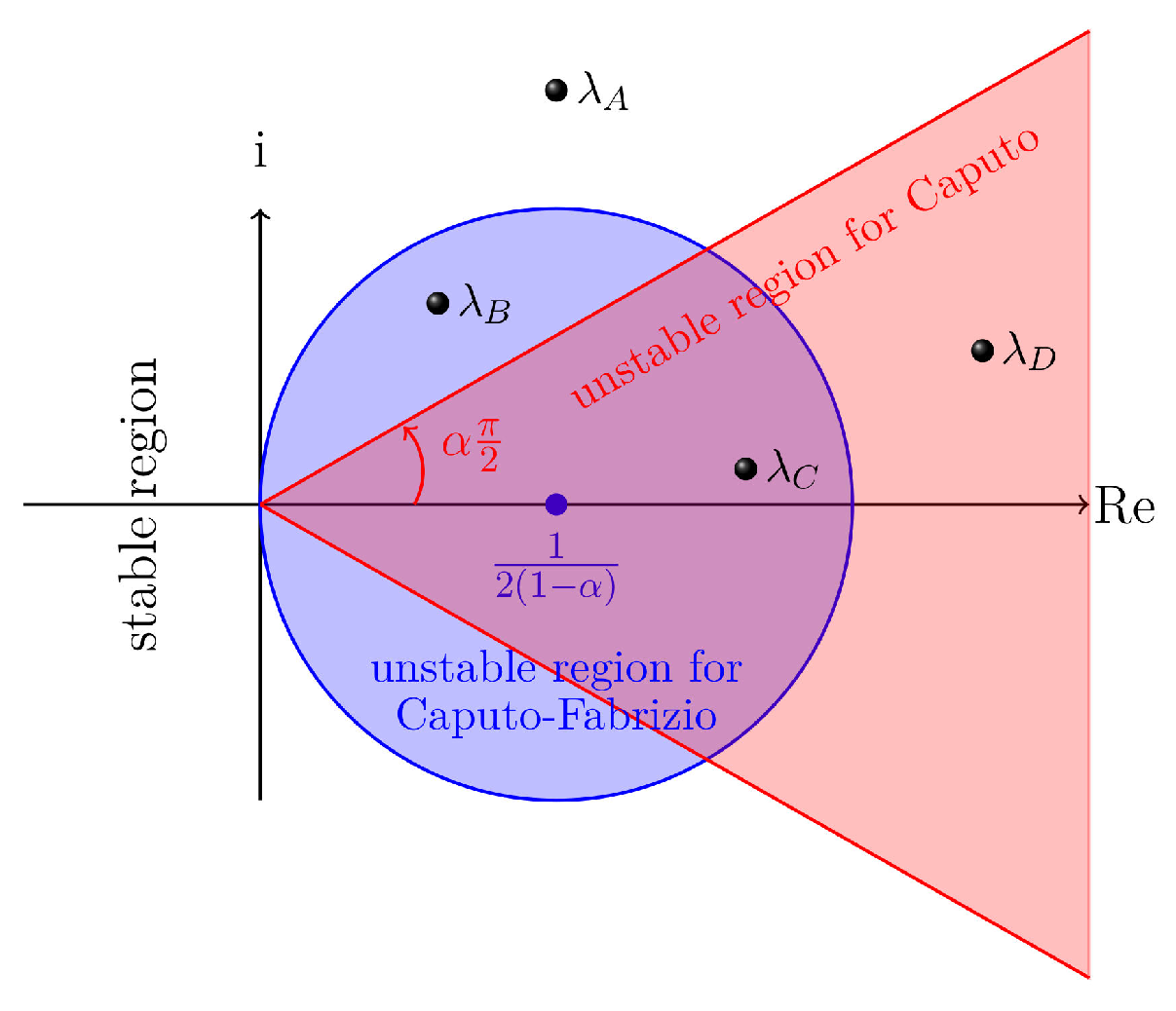
To illustrate such a classification, we provide stability and instability region for both operators in Figure 2 and set four eigenvalues on the plane for different cases. The unstable domain of the system with Caputo derivative is an unbound region limited by two lines with angles α π 2 and α π 2 . On the other hand, the unstable domain of the system with CF operator is a bounded closed circle centered at ( 0 , 1 2 ( 1 α ) ) with the radius 1 2 ( 1 α ) . For both cases, it is clear that the stability of the system has an inverse relation with the order derivative; in fact, the smaller the value of α , the more the region of stability and vice versa. As it is shown in Figure 2, the eigenvalues can be located in four distinct classes: λ A is in an area where both systems are stable; the class of λ B is where the system with Caputo derivatives is stable, but the system with CF operator is not stable; λ C denotes a class of eigenvalues staying at where both systems are unstable; and finally, λ D is where the system in the sense of CF operator is stable but the system with Caputo derivatives is not stable.
We collect a summary of the three examples in Table 3 to easily compare the behavior of the model concerning the Caputo and CF operators. These examples show different dynamical patterns over time, depending on the type of the operator and its stability landscape (Figure 2). In the following, we focus on the asymptotic stability of the different equilibria and further discuss general concepts in applied contexts.

6.1. Example 1

As one can see in Table 3, the parameters of this example give five distinct equilibrium points (and corresponding eigenvalues), where the equilibrium ϵ 4 is not acceptable since it has a negative value. Thus, we should expect negative-value solutions of the system when we do not impose any constraints on the components. We refer the readers to the technique used in [47] to avoid going toward such meaningless solutions and get a feasible solution.
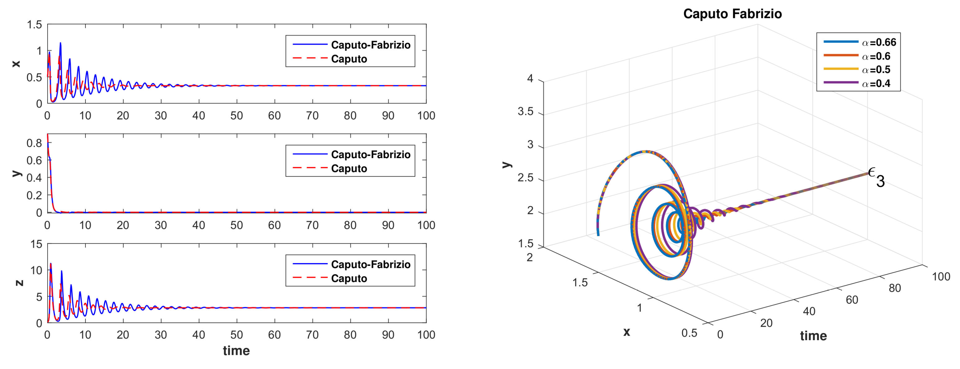
Furthermore, this example shows the stability of the equilibrium points depends on the value of the fractional-order α . As we expect from Figure 2, the number of stable equilibrium points increases when we reduce the value of α . In this case, when α is 0.98 for both operators, the system is asymptotically stable only at ϵ 2 (see Table 3). Indeed, Figure 3 (left) shows that the system gets steady at ϵ 2 , with different oscillations which are related to the definition of the operators. Nonetheless, the condition α 0.66 provides a larger area for the stability of the system with the CF operator so that three eigenvalues λ 0 , λ 1 , and λ 3 stay in the class of λ D (see Figure 2 and Table 3). Hence, with appropriate initial values and differential orders, the system with the CF operator could converge to ϵ 3 (see Figure 3, right) whereas the system with the Caputo operator is always unstable.

6.2. Example 2

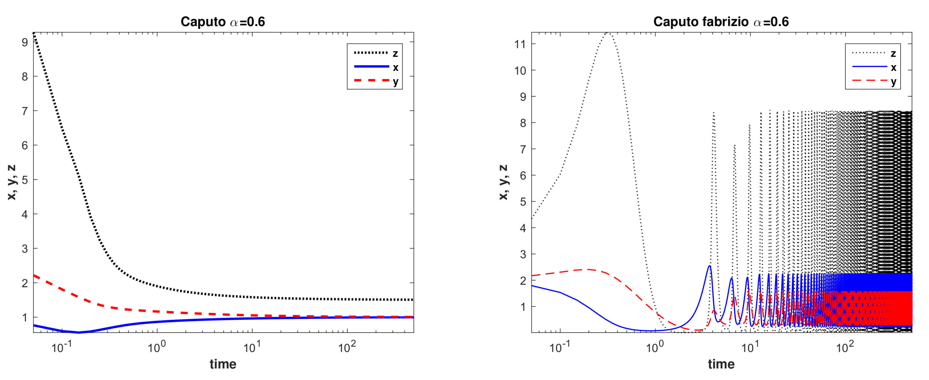
This example confirms the points mentioned in the previous one; By setting α = 0.6 , the equilibrium ϵ 4 is the only stable equilibrium point in the sense of Caputo derivative, while the equilibrium points ϵ 0 , ϵ 1 , and ϵ 3 are stable concerning the CF operator. But, as shown in Figure 2, it is interesting that we have here an eigenvalue, λ 4 , in the class of λ B alongside the λ D , where λ 0 , λ 1 , and λ 3 are. As a result, Figure 4 shows that the system can start from a point to converge asymptotically to the only equilibrium that is stable in the sense of Caputo, rather than the CF operator. Therefore, it could make a challenge for one who assumes a system with a more stability region may lead to more potential to achieve a steady-state.

6.3. Example 3

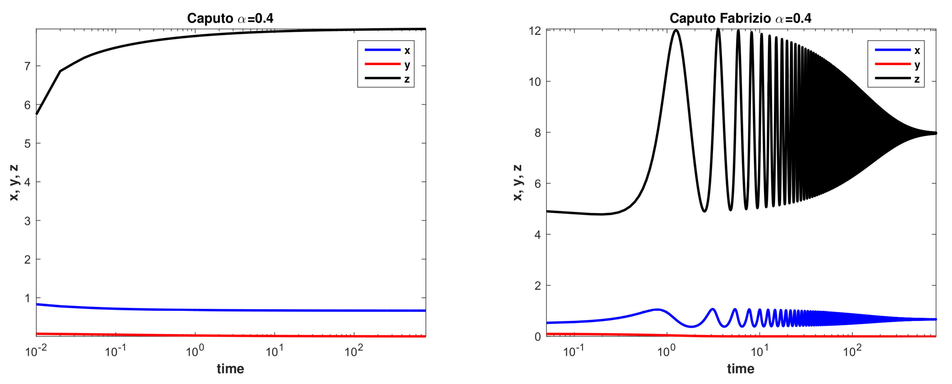
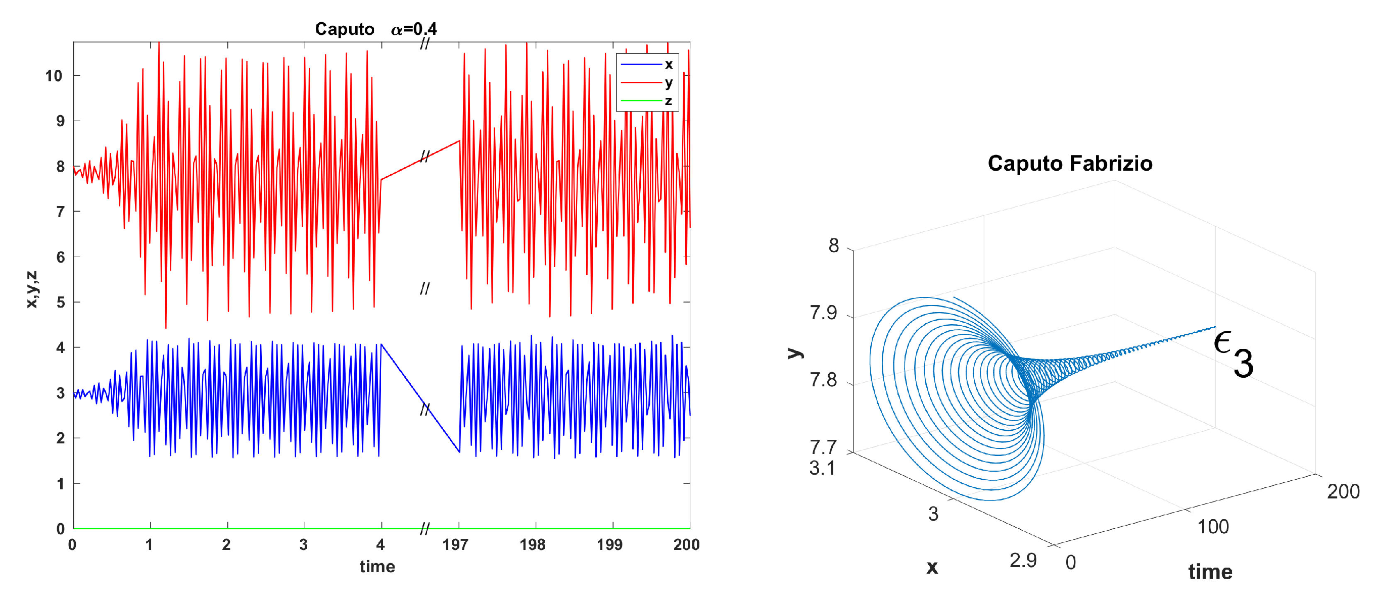
This example can complete the discussion and make clear the substantial role of the initial values on the behavior of our LV model. Considering the information in Table 3, determining the location of four eigenvalues in the λ D class (Figure 2), we expect that the system is most stable for the CF operator and noticeably unstable for the Caputo derivative. Although Figure 5 illustrates this expectation, it is not an absolute scenario when the process is supposed to start from a point leading to equilibrium ϵ 3 . It depends on the domain of attraction that the initial values stay and the corresponding eigenvalue, which is in the class of λ B (see Figure 6). For more information on finding the domain of attractions to specific equilibrium points, see [47].

6.4. Discussion

In the sense of ecological and biological contexts, the zero value of one variable of our LV model indicates the extinction of a species, and the system becomes a two-species community model. Hence, according to the number of interactions, the existence of the species x is crucial for an active dynamical system. The conditions given in Example 2 only lead to a coexistence of three species, whereas the last example starts with the interactions of two species and others converge to a two-species system.
The numerical results suggest that the fractional operator derivatives of a deterministic model can qualitatively affect the dynamic behavior (periodic/oscillations and asymptotically stable patterns), which is a significant outcome. For instance, Figure 5 shows a same convergence with different scenarios. On the other hand, in the real world, small environmental changes or any (external/internal) perturbations may alter the steady-state of a system community [35]. Consequently, a community described by the fractional LV models could be remarkably dependent on the type of the derivative operator. Furthermore, the purpose of using fractional operators in simulations or real data modeling is highly important. Tarasov [48] has shown that a system with the CF operator, in contrast to the Caputo fractional derivatives, cannot describe processes with memory effects but can suitably model processes with continuously distributed lag effects. Therefore, our results may represent distinct physical meanings of the LV model.

7. Conclusions

We have investigated the three-dimensional LV system for the CF operator. The toy model with the graph of the interactions have been illustrated to mention assumptions and applications of the system equation. Concerning the existence of a non-singular kernel in the definition of CF operator, we investigated the stability properties of the system with the CF fractional operator that have not been carried out in the context of nonlinear models.
A modified numerical method is suggested based on Adams-Bashforth methods. This numerical scheme simulate Caputo and CF operators, efficiently and numerical results demonstrate how the behavior of the LV system can depend on the type of differential operator and the value of fractional order. Moreover, we have shown that the CF operator provides different properties compared to the classical Caputo derivative and briefly mentioned the potential physical meanings. Overall, this analysis can enhance our understanding of the exceptional dynamics in complex systems. However, it is still demanding to discuss the biologically feasible region and boundedness of the system.
Analysing the behavior of LV models under incommensurate fractional orders, where the different interacting partners may have different degrees of memory or lag effects, is a fascinating line for further research. In real-world complex systems, a time-variable dependency on the past states is likely and may lead to anomalous behaviors that pose challenges for modeling. Besides, fractional calculus provides tools to simulate systems with such incommensurate fractional-order derivatives. Therefore, finding the stability region of the three-dimensional LV model with incommensurate fractional orders in the sense of Caputo and CF operators as well as examining the domain of attractions are promising directions for future studies.
Another idea for future research could be periodicity. When a critical point is a center and then the orbits are periodic in the classical model, the orbit related to this critical point loses the periodicity and form spirals in the fractional case. The issue of the periodicity of the solutions is a very important point in these systems because it is not clear if periodic orbits can exist in fractional cases especially for the CF operator.

Author Contributions

Conceptualization, M.K., L.E., S.H. and L.L.; Formal analysis, L.E.; Investigation, L.E.; Methodology, M.K. and S.H.; Software, M.K., L.E. and S.H.; Supervision, L.L.; Validation, L.L. All authors have read and agreed to the published version of the manuscript.

Funding

This research was funded by Academy of Finland (grants 295741, 330887).

Conflicts of Interest

The authors declare no conflict of interest.

References

  1. Sun, H.; Zhang, Y.; Baleanu, D.; Chen, W.; Chen, Y. A new collection of real world applications of fractional calculus in science and engineering. Commun. Nonlinear Sci. Numer. Simul. 2018, 64, 213–231. [Google Scholar] [CrossRef]
  2. Naik, P.A.; Owolabi, K.M.; Yavuz, M.; Zu, J. Chaotic dynamics of a fractional order HIV-1 model involving AIDS-related cancer cells. Chaos Solitons Fractals 2020, 140, 110272. [Google Scholar] [CrossRef]
  3. Kilbas, A.A.A.; Srivastava, H.M.; Trujillo, J.J. Theory and Applications of Fractional Differential Equations; Elsevier Science Limited: Amsterdam, The Netherlands, 2006; Volume 204. [Google Scholar]
  4. Podlubny, I. Fractional Differential Equations: An Introduction to Fractional Derivatives, Fractional Differential Equations, to Methods of Their Solution and Some of Their Applications; Elsevier: Amsterdam, The Netherlands, 1998. [Google Scholar]
  5. Naik, P.A.; Zu, J.; Owolabi, K.M. Global dynamics of a fractional order model for the transmission of HIV epidemic with optimal control. Chaos Solitons Fractals 2020, 138, 109826. [Google Scholar] [CrossRef] [PubMed]
  6. Karaagac, B.; Owolabi, K.M.; Nisar, K.S. Analysis and dynamics of illicit drug use described by fractional derivative with mittag-leffler kernel. CMC-Comput. Mater. Cont. 2020, 65, 1905–1924. [Google Scholar]
  7. Owolabi, K.M. High-dimensional spatial patterns in fractional reaction-diffusion system arising in biology. Chaos Solitons Fractals 2020, 134, 109723. [Google Scholar] [CrossRef]
  8. Owolabi, K.M. Computational techniques for highly oscillatory and chaotic wave problems with fractional-order operator. Eur. Phys. J. Plus 2020, 135, 1–23. [Google Scholar] [CrossRef]
  9. Saeedian, M.; Khalighi, M.; Azimi-Tafreshi, N.; Jafari, G.R.; Ausloos, M. Memory effects on epidemic evolution: The susceptible-infected-recovered epidemic model. Phys. Rev. E 2017, 95, 022409. [Google Scholar] [CrossRef] [PubMed] [Green Version]
  10. Ghalib, M.M.; Zafar, A.A.; Hammouch, Z.; Riaz, M.B.; Shabbir, K. Analytical results on the unsteady rotational flow of fractional-order non-newtonian fluids with shear stress on the boundary. Discret. Contin. Dyn. Syst.-S 2020, 13, 683. [Google Scholar]
  11. Baleanu, D.; Jajarmi, A.; Mohammadi, H.; Rezapour, S. A new study on the mathematical modelling of human liver with Caputo–Fabrizio fractional derivative. Chaos Solitons Fractals 2020, 134, 109705. [Google Scholar] [CrossRef]
  12. Caputo, M.; Fabrizio, M. A new definition of fractional derivative without singular kernel. Prog. Fract. Differ. Appl. 2015, 1, 1–13. [Google Scholar]
  13. Losada, J.; Nieto, J. Properties of a new fractional derivative without singular kernel. Prog. Fract. Differ. Appl. 2015, 1, 87–92. [Google Scholar]
  14. Caputo, M.; Fabrizio, M. Applications of new time and spatial fractional derivatives with exponential kernels. Prog. Fract. Differ. Appl. 2016, 2, 1–11. [Google Scholar] [CrossRef]
  15. Atangana, A.; Alkahtani, B. Controlling the wave movement on the surface of shallow water with the Caputo–Fabrizio derivative with fractional order. Chaos Solitons Fractals 2016, 89, 539–546. [Google Scholar]
  16. Moore, E.J.; Sirisubtawee, S.; Koonprasert, S. A Caputo–Fabrizio fractional differential equation model for HIV/AIDS with treatment compartment. Adv. Differ. Equ. 2019, 2019, 200. [Google Scholar] [CrossRef] [Green Version]
  17. Bushnaq, S.; Khan, S.A.; Shah, K.; Zaman, G. Mathematical analysis of HIV/AIDS infection model with Caputo-Fabrizio fractional derivative. Cogent Math. Stat. 2018, 5, 1432521. [Google Scholar] [CrossRef]
  18. Arshad, S.; Baleanu, D.; Defterli, O.; Shumaila. A numerical framework for the approximate solution of fractional tumor-obesity model. Int. J. Model. Simulation Sci. Comput. 2018, 10, 1941008. [Google Scholar] [CrossRef]
  19. Ortigueira, M.D.; Machado, J.T. A critical analysis of the Caputo–Fabrizio operator. Commun. Nonlinear Sci. Numer. Simul. 2018, 59, 608–611. [Google Scholar] [CrossRef]
  20. Loh, J.R.; Isah, A.; Phang, C.; Toh, Y.T. On the new properties of Caputo–Fabrizio operator and its application in deriving shifted Legendre operational matrix. Appl. Numer. Math. 2018, 132, 138–153. [Google Scholar] [CrossRef]
  21. Qureshi, S.; Rangaig, N.A.; Baleanu, D. New numerical aspects of Caputo-Fabrizio fractional derivative operator. Mathematics 2019, 7, 374. [Google Scholar] [CrossRef] [Green Version]
  22. Toh, Y.T.; Phang, C.; Loh, J.R. New predictor-corrector scheme for solving nonlinear differential equations with Caputo-Fabrizio operator. Math. Methods Appl. Sci. 2018, 42, 175–185. [Google Scholar] [CrossRef] [Green Version]
  23. Atangana, A.; Owolabi, K.M. New numerical approach for fractional differential equations. Math. Model. Nat. Phenom. 2018, 13, 3. [Google Scholar] [CrossRef] [Green Version]
  24. Das, S.; Gupta, P. A mathematical model on fractional Lotka–Volterra equations. J. Theor. Biol. 2011, 277, 1–6. [Google Scholar] [CrossRef]
  25. Calin-Adrian, C. Banking system: Three level Lotka-Volterra Model. Procedia Econ. Financ. 2012, 3, 251–255. [Google Scholar]
  26. Volterra, V. Variazioni e Fluttuazioni del Numero di Individui in Specie Animali Conviventi; Atti della R. Accademia Nazionale dei Lincei, C. Ferrari: Rome, Italy, 1927. [Google Scholar]
  27. Gonze, D.; Lahti, L.; Raes, J.; Faust, K. Multi-stability and the origin of microbial community types. ISME J. 2017, 11, 2159. [Google Scholar] [CrossRef] [Green Version]
  28. Ahmed, E.; El-Sayed, A.; El-Saka, H. Equilibrium points, stability and numerical solutions of fractional-order predator-prey and rabies models. J. Math. Anal. Appl. 2007, 325, 542–553. [Google Scholar] [CrossRef] [Green Version]
  29. Samardzija, N.; Greller, L.D. Explosive route to chaos through a fractal torus in a generalized Lotka-Volterra model. Bull. Math. Biol. 1988, 50, 465–491. [Google Scholar] [CrossRef]
  30. Elettreby, M.; Al-Raezah, A.A.; Nabil, T. Fractional-order model of two-prey one-predator system. Math. Probl. Eng. 2017, 2017, 1–12. [Google Scholar] [CrossRef] [Green Version]
  31. Owolabi, K.M. Numerical approach to chaotic pattern formation in diffusive predator–prey system with Caputo fractional operator. Numer. Methods Partial. Differ. Equ. 2021, 37, 131–151. [Google Scholar] [CrossRef]
  32. Naik, P.A.; Yavuz, M.; Qureshi, S.; Zu, J.; Townley, S. Modeling and analysis of COVID-19 epidemics with treatment in fractional derivatives using real data from pakistan. Eur. Phys. J. Plus 2020, 135, 1–42. [Google Scholar] [CrossRef]
  33. Amirian, M.M.; Towers, I.; Jovanoski, Z.; Irwin, A.J. Memory and mutualism in species sustainability: A time-fractional Lotka-Volterra model with harvesting. Heliyon 2020, 6, e04816. [Google Scholar] [CrossRef]
  34. Selvam, A.G.M.; Dhineshbabu, R.; Vianny, D.A. Analysis of a fractional order prey-predator model (3-species). Glob. J. Comput. Sci. Math. 2015, 5, 95–102. [Google Scholar]
  35. Gonze, D.; Coyte, K.Z.; Lahti, L.; Faust, K. Microbial communities as dynamical systems. Curr. Opin. Microbiol. 2018, 44, 41–49. [Google Scholar] [CrossRef]
  36. Eklöf, A.; Ebenman, B. Species loss and secondary extinctions in simple and complex model communities. J. Anim. Ecol. 2006, 75, 239–246. [Google Scholar] [CrossRef] [PubMed]
  37. Haerter, J.O.; Mitarai, N.; Sneppen, K. Food web assembly rules for generalized Lotka-Volterra equations. PLoS Comput. Biol. 2016, 12, 1–17. [Google Scholar] [CrossRef] [PubMed]
  38. Kreyszig, E. Introductory Functional Analysis with Applications; Wiley: New York, NY, USA, 1978; Volume 1. [Google Scholar]
  39. Hunter, J.K.; Nachtergaele, B. Applied Analysis; World Scientific: Singapore, 2001. [Google Scholar]
  40. Conway, J.B. A Course in Functional Analysis; Springer: Berlin/Heidelberg, Germany, 2019; Volume 96. [Google Scholar]
  41. Yavuz, M.; Sene, N. Stability analysis and numerical computation of the fractional predator–prey model with the harvesting rate. Fractal Fract. 2020, 4, 35. [Google Scholar] [CrossRef]
  42. Matignon, D. Stability results for fractional differential equations with applications to control processing. Comput. Eng. Syst. Appl. 1996, 2, 963–968. [Google Scholar]
  43. Li, H.; Cheng, J.; Li, H.b.; Zhong, S.R.M. Stability analysis of a fractional-order linear system described by the Caputo-Fabrizio Derivative. Mathematics 2019, 7, 200. [Google Scholar] [CrossRef] [Green Version]
  44. Garrappa, R. On linear stability of predictor–corrector algorithms for fractional differential equations. Int. J. Comput. Math. 2010, 87, 2281–2290. [Google Scholar] [CrossRef]
  45. Diethelm, K.; Ford, N.J.; Freed, A.D. A predictor-corrector approach for the numerical solution of fractional differential equations. Nonlinear Dyn. 2002, 29, 3–22. [Google Scholar] [CrossRef]
  46. Dadras, S.; Momeni, H. Control of a fractional-order economical system via sliding mode. Phys. A Stat. Mech. Its Appl. 2010, 389, 2434–2442. [Google Scholar] [CrossRef]
  47. Najafi, E.; Babuska, R.; Lopes, G. A fast sampling method for estimating the domain of attraction. Nonlinear Dyn. 2016, 86, 823–834. [Google Scholar] [CrossRef] [Green Version]
  48. Tarasov, V.E. Caputo–Fabrizio operator in terms of integer derivatives: Memory or distributed lag? Comput. Appl. Math. 2019, 38, 113. [Google Scholar] [CrossRef]
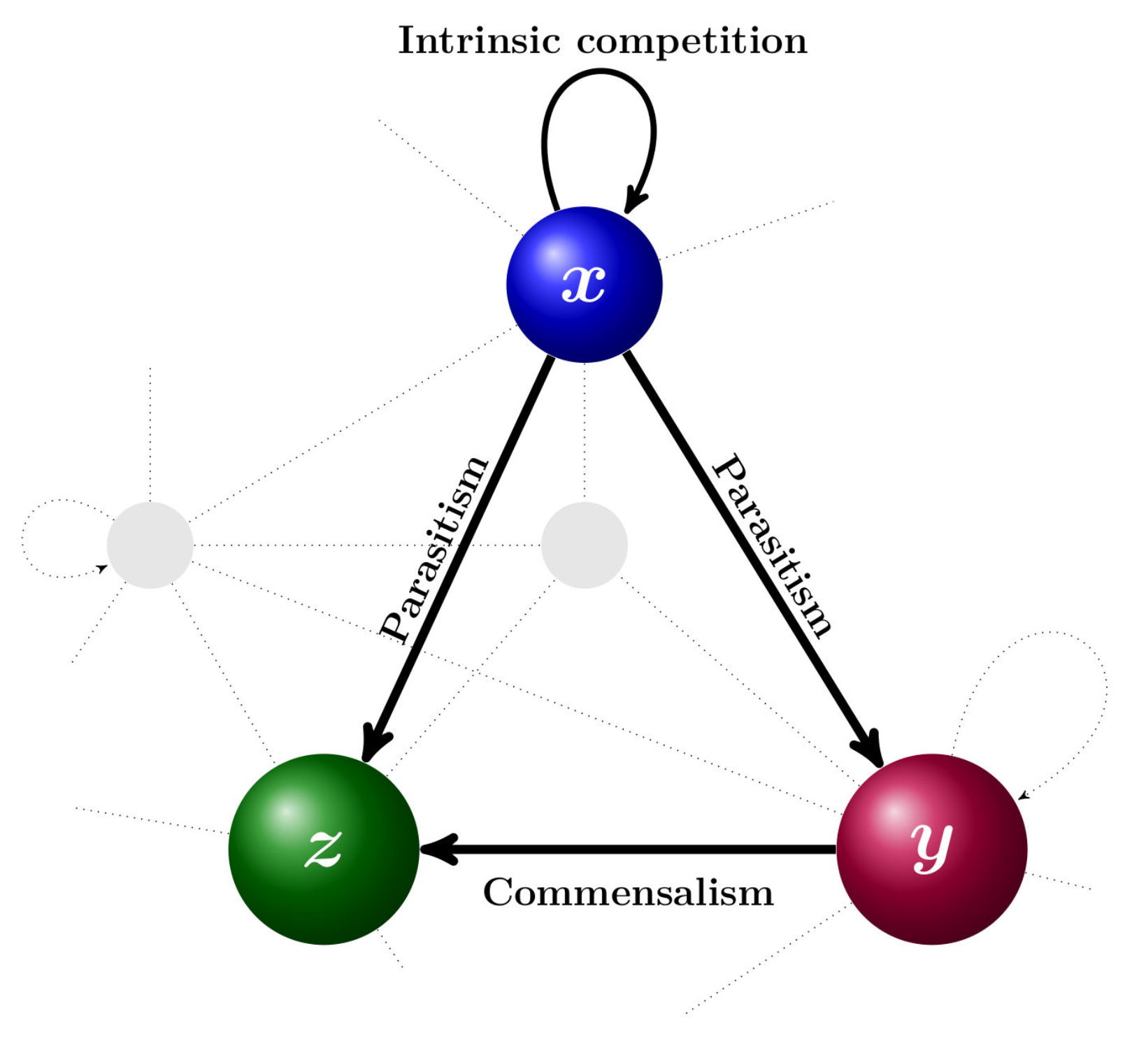
Figure 1. Simulation model for the interactions of a three-species community represented by Equation (7). The system is isolated for three species and does not depend on interactions with the other species (colorless background).
Symmetry 13 00368 g001
Figure 2. Comparison stability and unstability domain of Caputo and CF operators.
Symmetry 13 00368 g002
Figure 3. (left) Comparing the behavior of the Caputo and the CF operators for system (7) with the parameters of Example 1, (right) converging to ϵ 3 with CF operator for α 0.66 and ( x 0 , y 0 , z 0 ) = ( 1.6 , 1.9 , 0 ) .
Symmetry 13 00368 g003
Figure 4. System (7) with the parameters of Example 2 and ( x 0 , y 0 , z 0 ) = ( 2 , 2 , 3 ) is asymptotically stable for Caputo (left) and unstable for CF (right).
Symmetry 13 00368 g004
Figure 5. System (7) with the parameters of the Example 3 and ( x 0 , y 0 , z 0 ) = ( 0.5 , 0.1 , 5 ) is asymptotically stable for both Caputo (left) and CF (right) at ϵ 2 with different oscillations.
Symmetry 13 00368 g005
Figure 6. System (7) with the parameters of the Example 3 and ( x 0 , y 0 , z 0 ) = ( 3 , 8 , 0 ) , α = 0.4 , t = 200 is unstable for Caputo (left) and asymptotically stable for CF (right).
Symmetry 13 00368 g006
Table 1. Required conditions for the existence of the equilibrium points.
Equilibrium PointsConditions
ε 0 Always exists
ε 1 Always exists
ε 2 a 5 1 and a 1 a 6 a 2 ( a 5 1 )
ε 3 a 3 1 and a 1 a 4 a 2 ( a 3 1 )
ε 4 a 3 1 , a 4 ( a 5 1 ) a 6 ( a 3 1 ) and a 4 ( a 2 a 7 a 6 ) ( a 3 1 ) ( 1 + a 1 a 7 a 5 )
or
( 1 + a 1 a 7 a 5 ) < 0 , a 4 ( a 6 a 2 a 7 ) ( a 3 1 ) ( 1 + a 1 a 7 a 5 )
or
1 + a 1 a 7 a 5 = 0 and a 6 > a 2 a 7
Table 2. Stability conditions for Caputo and Caputo-Fabrizio (CF) operators.
Fixed PointsCaputo DerivativeCF Operator
ε 0 Always saddle a 1 > 1 1 α
ε 1 a 1 a 2 < a 2 a 3 a 2    and   a 1 a 2 < a 2 a 3 a 2 a 1 a 2 < a 2 a 3 a 2 and a 1 a 2 < a 2 a 3 a 2
or
a 1 a 4 a 2 a 3 a 2 > α 1 α   and   a 1 a 6 a 2 a 5 a 2 > α 1 α
ε 2 a 5 1 a 6 < a 1 a 2 < a 3 1 a 4 a 5 1 a 6 < a 1 a 2 < a 3 1 a 4
or
1 a 3 a 4 a 6 ( 1 a 5 ) > 1 1 α   and a 2 ( 1 a 5 ) ± a 2 2 ( 1 a 5 ) 2 + 4 a 6 ( 1 a 5 ) ( a 1 a 6 + a 2 ( 1 a 5 ) ) > 2 a 6 1 α
ε 3 a 3 1 a 4 < a 1 a 2 < a 5 1 a 6 a 3 1 a 4 < a 1 a 2 < a 5 1 a 6
or
1 a 4 a 6 a 4 ( 1 a 3 ) + a 7 a 4 [ a 1 a 4 + a 2 ( 1 a 3 ) ] > 1 1 α    and a 2 ( 1 a 3 ) ± a 2 2 ( 1 a 3 ) 2 + 4 a 4 ( 1 a 3 ) [ a 1 a 4 + a 2 ( 1 a 3 ) ] > 2 a 4 1 α
ε 4 a 6 > a 2 a 4 ( a 3 1 ) [ w + a 2 ( a 3 1 ) ] w ( a 2 + a 4 ) + a 2 a 4 ( a 3 1 ) w = a 4 ( 1 + a 1 a 7 a 5 ) + ( a 6 a 1 a 7 ) ( a 3 1 ) a 6 > a 2 a 4 ( a 3 1 ) [ w + a 2 ( a 3 1 ) ] w ( a 2 + a 4 ) + a 2 a 4 ( a 3 1 )
or
λ 1 , λ 2 , λ 3 > 1 ( 1 α )
(see Equations (48)–(50))
Table 3. The summary of examples; C, CF, and U ( 0 ) denote Caputo, Caputo-Fabrizio, and initial values, respectively, and the notation ✓ indicates the system is asymptotically stable, while ✗ implies unstability.
Example 1CCFCCF
Coefficient U ( 0 ) EquilibriumEigenvalues α = 0.98 α 0.66
a 1 = 3
a 2 = 0.5
a 3 = 4
a 4 = 3
a 5 = 4
a 6 = 9
a 7 = 4
x 0 = 0.5
y 0 = 0.9
z 0 = 0.1
ε 0 ( 0 , 0 , 0 ) λ 0 ( 3 , 3 , 3 )
ε 1 ( 6 , 0 , 0 ) λ 1 ( 3 , 15 , 51 )
ε 2 ( 0.33 , 0 , 2.83 ) λ 2 ( 0.083 2.914 i , 0.083 + 2.914 i , 2 )
ε 3 ( 1 , 2.5 , 0 ) λ 3 ( 0.25 2.727 i , 0.25 + 2.727 i , 16 )
ε 4 ( 1 , 1.5 , 4 ) Not Acceptable λ 4 ( 1.239 5.904 i , 1.239 + 5.904 i , 1.978 )
Example 2CCF
Coefficient U ( 0 ) EquilibriumEigenvalues α = 0.6
a 1 = 3
a 2 = 0.5
a 3 = 4
a 4 = 3
a 5 = 14
a 6 = 9
a 7 = 4
x 0 = 2
y 0 = 2
z 0 = 3
ε 0 ( 0 , 0 , 0 ) λ 0 ( 13 , 3 , 3 )
ε 1 ( 6 , 0 , 0 ) λ 1 ( 3 , 15 , 41 )
ε 2 ( 1.44 , 0 , 2.28 ) λ 2 ( 0.361 5.429 i , 0.361 + 5.429 i , 1.333 )
ε 3 ( 1 , 2.5 , 0 ) λ 3 ( 0.25 2.727 i , 0.25 + 2.727 i , 6 )
ε 4 ( 1 , 1 , 1.5 ) λ 4 ( 0.276 4.123 i , 0.276 + 4.123 i , 1.053 )
Example 3CCF
Coefficient U ( 0 ) EquilibriumEigenvalues α = 0.4
a 1 = 8
a 2 = 0.5
a 2 = 4
a 4 = 1
a 5 = 7
a 6 = 9
a 7 = 4
x 0 = 0.5
y 0 = 0.1
z 0 = 5
ε 0 ( 0 , 0 , 0 ) λ 0 ( 6 , 3 , 8 )
ε 1 ( 160 , 0 , 0 ) λ 1 ( 8 , 157 , 1434 )
ε 2 ( 0.666 , 0 , 7.966 ) λ 2 ( 0.016 6.913 i , 0.016 + 6.913 i , 2.333 )
ε 3 ( 3 , 7.85 , 0 ) λ 3 ( 0.075 4.852 i , 0.075 + 4.852 i , 52.4 )
ε 4 ( 3 , 5.25 , 13.1 ) Not Acceptable λ 4 ( 1.274 18.50 i , 1.274 + 18.50 i , 2.398 )
Publisher’s Note: MDPI stays neutral with regard to jurisdictional claims in published maps and institutional affiliations.