Sensitivity Analysis of the Optimal Inventory-Pooling Strategies According to Multivariate Demand Dependence

Abstract

Inventory-pooling (IP) is an effective tool to mitigate demand uncertainty and variability, to reduce operational costs, and consequently to increase the profit. The major assumptions of the previous works in literature on IP include the following: (1) Independents demand, which satisfy the typical normal independent and identically distributed (iid) random variables; (2) dependents (correlated) symmetric demands, which follows to a multivariate normal distribution. The effect of the dependent asymmetric demand is not yet studied. The aim of this paper is to consider this more realistic case. Indeed, the contribution of this paper is twofold. Firstly, it analyzes both the sensitivity of dependence structure and the levels of skewness of distributions on IP policies in terms of optimal total cost and demand satisfaction constraint. Secondly, both symmetric and asymmetric demand distributions are modeled using various beta distribution and the dependance between demands are modeled using various copulas. A newsvendor problem inspired by the literature, with two decentralized locations and two centralized locations, is considered the empirical study. For each dependance situation, three IP models are considered: inventory centralization, regular transshipments, and independent systems. The results suggest divergences in the decisions in about 9% of cases. Bad choice of marginal distributions given that the copula is appropriate can lead to divergences that vary between 2.2% and 4%, depending on whether the demand distributions are symmetric or asymmetric.

1. Introduction

Inventory management is a crucial component in controlling costs and ensuring delivery to customers with minimal delays and interruptions [1]. Uncertainty represents one of the most critical issues facing firms around the world [2]. Indeed, studying uncertainty of demand is a key aspect for each firm’s inventory management. Inventory-pooling (IP) is a technique that is widely used to cope with supply chain uncertainty. In the literature, there many other names referred to as IP, such as inventory consolidation, portfolio effect, consolidation effect, etc. Whichever name is used, it is a good practice for minimizing risks of follow-on demand uncertainty and therefore decreasing inventory cost. It can be achieved in numerous policies, including inventory centralization [3], transshipments [4], postponement, order splitting, etc. Often, savings arising from pooling are defined based on an independent system where each retailer is disserved exclusively by a manufacturer.

This research concerns two studied problem areas in the literature: demand pooling and demand dependence. An extensive literature has focused on the demand pooling problem under general demand dependence and demand distributions. In the literature on IP, researchers mainly focus on comparison in terms of profit (or cost) between a decentralized system and several forms of centralized system. For a detailed review, the reader can consult many references such as Schmitt [5], Schmitt et al. [6], Thomas and Tyworth [7], etc. One of the earliest works in this area is the newsboy model with multiple sources of demand, which is proposed by Eppen [8]. He considered the benefits of consolidation assuming regular or negligible transportation costs. Some other researchers focus on comparison between pooling and no pooling cases in terms of inventory level. The reader can consult the works of Alfaro and Corbett [9] and Bimpikis and Markakis [10] for a detailed review. The proposed research is interested in comparison between a decentralized system and several forms of centralized system (centralization inventory and transshipments) in terms of optimal total cost.

A key assumption usually in literature is that demands are typical normal independent and identically distributed (iid) random variables, such as in Tyagi and Das [3], Evers and Beier [11], Evers [12], Schmitt et al. [6], Axsäter [13], Lee [14], Rojas et al. [15], etc. However, global demand is the total sum of individual demands from several customers; it is the sum of n random variables (n is the number of customers) that is not independent and eventually does not follow to the same distribution. Inventory and production levels are determined on the basis of global demand in a way that is ignorant of dependence between individual demands. This affects decisions and strategies of the supplier and implies under or overestimation of inventory level. Moreover, in literature dealing with inventory centralization and transshipments, the impact of dependence in optimal inventory level and costs has been studied assuming correlated multivariate normal demand. This assumption not verified in practice, remains restrictive, and implies under or overestimation of inventory level. However, a few studies in literature, such as Aydin et al. [16], Silbermayr et al. [17], and Wanke [18] have criticized the normality and independence assumption. Aydin et al. [16] studied the effect of inventory centralization on the optimal inventory level by performing a sensitivity analysis showing the effect of centralization on the efficiency of each of the following factors: the marginal ratio, the demand distribution as well as the asymmetry coefficient, the Kendall rate, and the copula chosen to model the dependence structure. Silbermayr et al. [17] determined the optimal pooling policies to minimize inventory level and maximize the benefit under an environmental constraint based on carbon emissions. They discussed the sensitivity of demand distributions and dependence structure with respect to cost and emissions. Wanke [18] offers an interesting sensitivity of normal demand dependence on optimal cost and demand satisfaction constraint.

In this paper, these three previous works [16,17,18] are extended. Both the impact of dependence structure and the levels of skewness of such distributions on cost and demand satisfaction constraint with beta demand distribution are analyzed. Therefore, this study is interested in dependence structures using copulas to generate multivariate joint distributions. Indeed, copula is a very powerful mathematical tool in multivariate modeling. This allows us to assess the impact of different (linear and non-linear) tail dependence of demands for any type of marginal demand distributions on decision-making within pooling models (centralization pooling and transshipments).

It should be noted that in this research, optimal IP strategy is sought. However, in the literature, there are many taxonomies to classify optimization problems and models: deterministic or stochastic, static or dynamic, discrete or continuous, linear or non-linear, etc. This paper presents a sensitivity analysis of the optimal selection of the adequate IP strategies according to multivariate demand dependence. Therefore, the type of the optimization used here is stochastic and nonlinear, but it is a discrete optimization, all used variables are fixed periodically on time, and it involves a finite-dimensional decision space only.

The aim of this paper is to show how both a good modeling of demands dependence structure and a best choice of demand distributions allow the taking of the selection of the best pooling model. Moreover, the majority of the pooling results and using copulas rely on the assumption that the marginal demand follows a normal (symmetric) distribution such as in Wanke [18] and Corbett and Rajaram [19]. When the beta distribution is used, the behavior of both symmetric and asymmetric distribution is modelled. Moreover, the different allocation rules, namely those proposed by Tyagi and Das [3] and Ballou and Burnetas [4], are considered. The objective is to discuss the asymmetrical impact of distribution on such decisions. Indeed, different levels of skewness of distributions for different options of IP under general demand dependence are studied. On one hand, the dependence structure between demands is modeled and simulated using copulas, and on the other hand, both symmetric and asymmetric demand distributions are studied using various beta distribution. Different IP policies under general demand dependence incorporating a demand satisfaction constraint are compared.

This work studies the degree of sensitivity of the choice decision of one of the transshipments, independence, or centralization policies to the chosen copula to model the dependence. In particular, for these consolidation effect models, the implications of these uncertainties are studied, and answers research questions include the following. (1) What are the most influential variables in choosing the optimal pooling model? (2) What is the degree of sensitivity results to the choice of the distribution demand? To the skewness asymmetry coefficient of this distribution? (3) What is the degree of sensitivity results to the choice of the dependence structure (choice of the copula)?

2. Costs and Inventory Pooling Stetting

2.1. Total Cost in Consolidation Setting

According to Wanke and Saliby [20] and Wanke [21], the total cost analysis (TC) in IP considers the sum of three components: the cycle stock cost (CSc), the safety stock cost (SSc) and the distribution cost (DC).

2.1.1. The Cycle Stock Cost

The cycle stock (CSc) is the result of the inventory consolidation from multiple n locations (or stocking points that serve demand) into a fewer number of m locations (where $\ge m\ge 1$). The expression of this cost at m centralized locations is given by Evers [6] as mentioned in Equation (1)

$$CSc=\frac{1}{2}·{\displaystyle \sum }_{f=1}^{m}EO{Q}_f$$

(1)

where $EO{Q}_f$ denotes the economic order quantity at centralized location f, and expressed according to the Equation (2).

$$EO{Q}_f=\sqrt{2·\frac{P_f}{h_f}·E\left({\displaystyle \sum }_{i=1}^n\left(W_{i,f}·D_i\right)\right)}$$

(2)

where:

• D_i: is the mean demand during one time period at decentralized location i,
• P_f: is the fixed order processing cost at centralized location f ($ per order),
• h_f: is the unitary inventory holding cost per time period at centralized location f ($ per day), and
• W_i,f: is the proportion of mean demand during one time period transferred from decentralized location i to centralized location f (where $0\le W_{i,f}\le 1,$ for all i and f, and ${\sum }_{f=1}^m{W}_{i,f}=1,$ for all i).

2.1.2. The Safety Stock Cost

The total safety stock at m centralized locations, as a result of the inventory consolidation (SSc) from n decentralized locations is given by Evers and Beier [5] and shown in Equation (3).

$$SSc=k{\displaystyle \sum }_{f=1}^m{\sigma }_f=k·{\displaystyle \sum }_{f=1}^m\sqrt{E{\left({\displaystyle \sum }_{i=1}^n{W}_{i,f}·D_i\right)}^2·s_{LT,f}^2+V\left({\displaystyle \sum }_{i=1}^n{W}_{i,f}·D_i\right)·E\left(L{T}_f\right)}$$

(3)

where:

• LT_f: is the mean lead time at centralized location f;
  S_{LT, f}: is the standard deviation of lead time at centralized location f;
• k: is the safety stock factor;
• ρ_ij: is the correlation of demand between decentralized locations i and j;
• S_{D, i}: is the standard deviation of demand during one period at decentralized location i;
• σ_f: is the standard deviation of demand at centralized location f during the lead time period;
• E(): random variable expectation; and
• V(): random variable variance.

$$V\left({\displaystyle \sum }_{i=1}^n{W}_{i,f}·D_i\right)=\left[\left({\displaystyle \sum }_{i=1}^n{W}_{i,f}^2·s_{D,i}^2\right)+2\left({\displaystyle \sum }_{i=1}^n{\displaystyle \sum }_{j=1}^{i-1}{W}_{i,f}{W}_{j,f}{\rho }_{ij}{s}_{D,i}{s}_{D,j}\right)\right]$$

(4)

It should be noted that σ_f is the standard deviation of a compound distribution while k represents the quantile of this distribution. The final expression of σ_f is shown in Equation (5).

$${\sigma }_f=\sqrt{E{\left({\displaystyle \sum }_{i=1}^n{W}_{i,f}·D_i\right)}^2·s_{LT,f}^2+V\left({\displaystyle \sum }_{i=1}^n{W}_{i,f}·D_i\right)·E\left(L{T}_f\right)}$$

(5)

Equation (5) remains valid only in the case of the following five assumptions: (1) All actors use the safety factor approach ((k.s) with s representing the standard deviation of demand during the lead time) to determine the level of security stock before and after consolidation; (2) all actors use the same security stock factor to achieve the desired level of service; (3) all players adopt the Economic Order Quantity (EOQ) approach to determine the quantity ordered and the ROP (reorder point) approach for inventory control; (4) the average total demand for the entire system remains the same after consolidation; And (5) lead time and demand are independent random variables.

2.1.3. The Distribution Cost

The total distribution cost is given by the Equation (6):

$$DC={\displaystyle \sum }_{f=1}^m{\displaystyle \sum }_{i=1}^n{d}_{f,i}·W_{i,f}·D_i$$

(6)

where d_f,i is the distribution cost rate, representing the unitary transportation of a single item from a centralized location f to a decentralized location i.

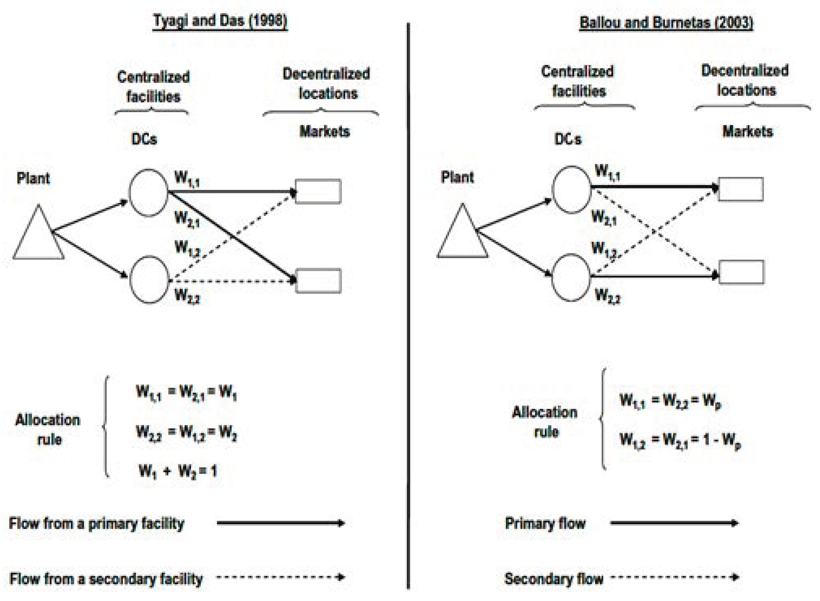
2.2. Demand Allocation Rules and Inventory Pooling Models

In the related literature on consolidation area, there are two different ways to satisfy the potential demand, as described in Figure 1:

-

Either all centralized locations offer the same proportion of demand at each decentralized location [3];

-

or a first source will be in charge of satisfying the demand and in case of lack a second source intervenes to satisfy the rest of this demand [4]. Figure 1 describes the difference between the two studied rules: Tyagi and Das’ allocation rule and Ballou and Burnetas’ allocation rule.

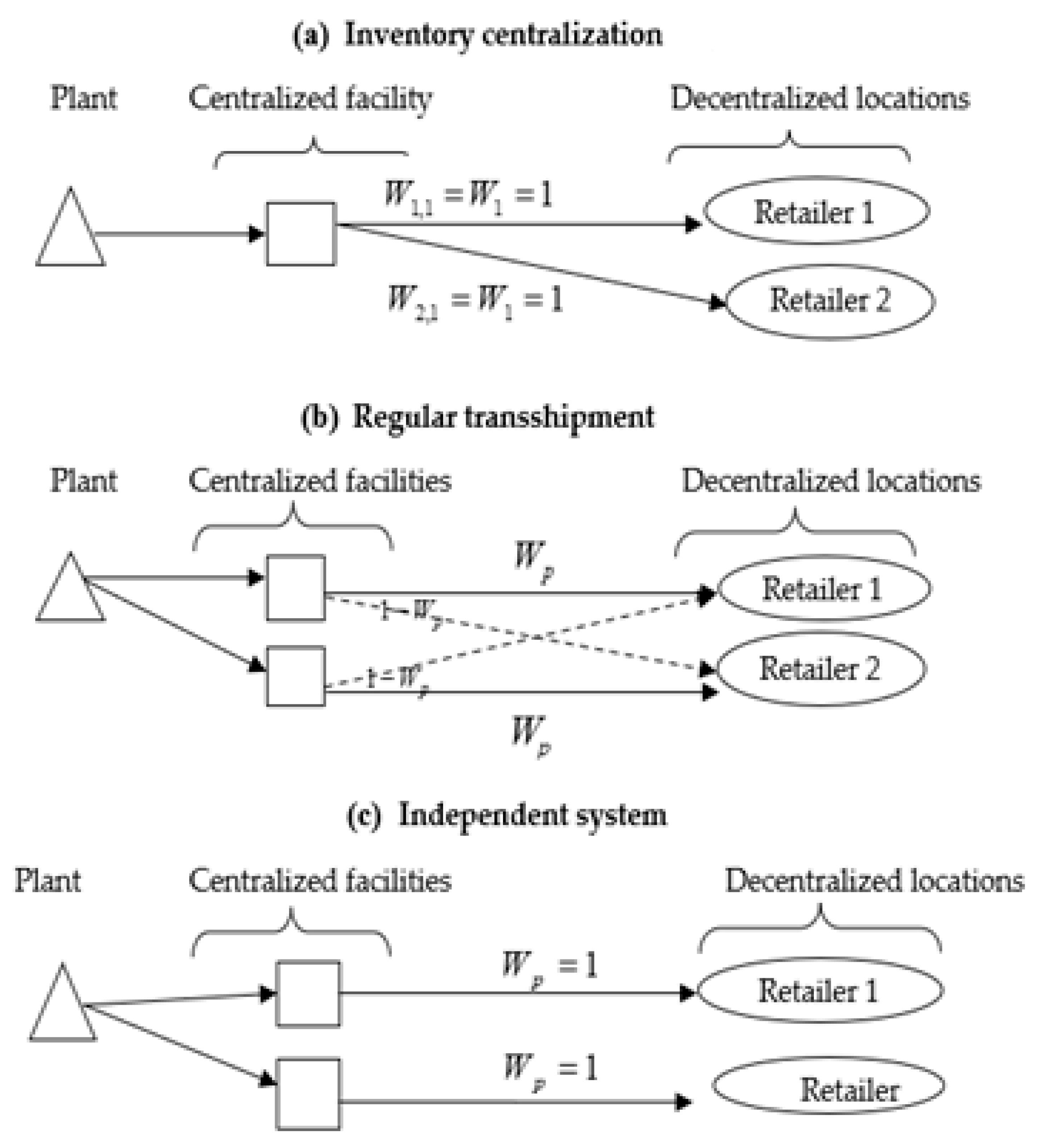
2.2.1. Tyagi and Das’ Allocation Rule (Inventory Centralization)

According to this allocation approach, the consolidation effect depends on the conditions of the lead times between the different locations. For centralized locations with means and variances of equal lead times, the fraction of demands to be offered for each decentralized location must be equal and they range from 0 to 1. Otherwise (difference in means or/and variances), the consolidation effect is greatest when inventories are centralized in one location [21]. Indeed, the condition that a centralized location offers the same fraction of the demand for each decentralized location is satisfied once that fraction is equal to one. The fractions of the demand must verify the following relation: $W_{1,f}=W_{2,f}=\dots =W_{n,f}=W_f$ for each I with $0\le W_f\le 1$ and ${\sum }_{f=1}^m{W}_f=1$.

In the case where it is equal to 0 or 1 at the optimum, the different decentralized locations will be served by a single central location (centralization policy/one delivery source).

2.2.2. Ballou and Burnetas’ Allocation Rule (Regular Transshipments or Independent Systems)

Under Ballou and Burnetas’ allocation rule, the demand for a storage location depends on the demand of its primary decentralized location but also on demands from other storage locations that are unable to meet the needs of their decentralized locations. Indeed, each centralized location f must provide the same fraction of the demand for its decentralized location i as the others while respecting the condition: $W_{1,1}=W_{2,2}=W_p$ and $W_{1,2}=W_{2,1}=1-W_p$.

The index p indicates the primary location for each centralized location. In the case where $W_p$ is equal to 0 or 1 at the optimum, each decentralized location will be served exclusively by a single centralized location (independent distribution system). This means that there is no point in applying a centralized system where only one location takes over the responsibility of serving all decentralized locations [22].

In the case where $W_p$ is between 0 and 1, it is preferable to apply a regular transshipment policy. This means that all decentralized locations will be served by all centralized locations. A value between 0 and 1 may result in the same policy being applied according to the allocation formula of Tyagi and Das [3], but this solution is not always optimal [20].

2.2.3. Linking Allocation Rules to Inventory Pooling Models

Several authors such as Tyagi and Das [3], Ballou and Burnetas [4], Corbett and Rajaram [19], Wanke and Saliby [20], Wanke [18], and Wanke [21,22] consider the particular case where $n=m=2$. In this paper, the presented results also concern the same case (two decentralized locations and two centralized locations). Demands are assumed to be positive random variables, D₁ and D₂, with a cumulative distribution functions F_D1 and F_D2, respectively. The centralized decision maker places an order at the manufacturer before observing demand.

Three IP strategies are considered in this research as described in Figure 2: Two types of pooling systems which including demand satisfaction constraints (allocation rules), and the third strategy is about an independent (no pooling) system. The first IP policy is the inventory centralization. It is the consolidation of inventory at decentralized locations in order to meet different demands and reduce expected costs as part of a cost minimization model or to increase profits and service levels in a profit maximization model [23]. In other words, a given centralized facility supplies the same fraction of demand to each decentralized location, like in Tyagi and Das [3].

The second IP policy is transshipment strategy. The main role of transshipment is the transfer of stocks between two entities in the same level of the supply chain. On a regular basis, transshipment implies that the transfer is from entity that is overstocked to entity which is in rupture. It involves organizing stock transfers between sites at the same level, either using a preventive approach to reduce the risk of disruption to customer demands, or using an emergency approach to resolve cases of actual disruption. Research on transshipment in literature is carried out under various settings. Evers [24,25,26] and Ballou and Burnetas [4] study transshipments pooling with the portfolio and the consolidation effects.

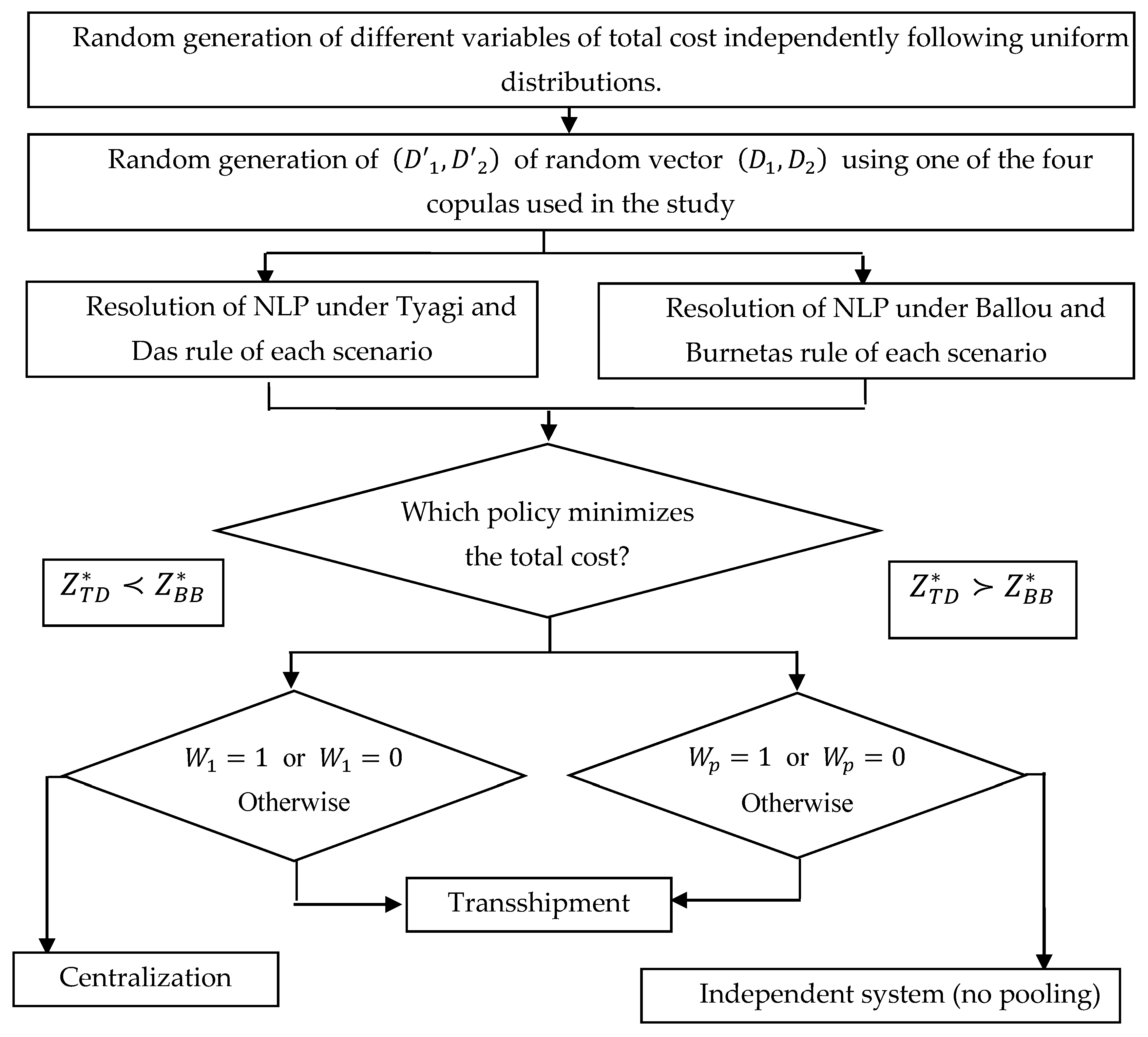
3. The Proposed Approach

3.1. Optimal Decision Search

The proposed approach is described in Figure 3. Since the optimum value of Wp cannot be analytically evaluated by solving the total cost derivative (with respect to Wp) for different conditions of demand and lead time, two types of non-linear programming were performed with software R. The models of the non-linear problem (NPL), are given in Equations (7) and (8). The programming model related to that of Ballou and Burnetas’ allocation rule is presented in Equation (7). The optimal function of the minimum cost for this rule is noted by $Z_{BB}^{*}$.

$$\begin{array}{c}\mathrm{Min} (k\sqrt{{\left(W_p{D}_1+\left(1-W_p\right)D_2\right)}^2·s_{LT,1}^2+\left(W_p^2·s_{D,1}^2+{\left(1-W_p\right)}^2·s_{D,2}^2+2W_P\left(1-W_p\right){\rho }_{1,2}{s}_{D,1}{s}_{D,2}\right)·L{T}_1}+\\ k\sqrt{{\left(\left(1-W_p\right)D_1+W_p{D}_2\right)}^2·s_{LT,2}^2+\left(·{\left(1-W_p\right)}^2{s}_{D,1}^2+W_p^2·s_{D,2}^2+2W_p\left(1-W_p\right){\rho }_{1,2}{s}_{D,1}{s}_{D,2}\right)·L{T}_2}+\\ \frac{\sqrt{2}}{2}\sqrt{\frac{\left(W_p{D}_1+\left(1-W_p\right)D_2\right)P_1}{h}}+\frac{\sqrt{2}}{2}\sqrt{\frac{\left(\left(1-W_p\right)D_1+W_p{D}_2\right)P_2}{h}})h+\left(d_{11}{W}_p+d_{21}\left(1-W_p\right)\right)D_1+\\ \left(d_{12}\left(1-W_p\right)+d_{22}{W}_p\right)D_2\\ \mathrm{subject}\mathrm{to}:0\le W_p\le 1.\end{array}$$

(7)

The programming model related to Tyagi and Das’ allocation rule is presented in Equation (8). The optimal function of the minimum cost for this rule is noted by $Z_{TD}^{*}$.

$$\begin{array}{c}\mathrm{Min}(k\sqrt{{\left(W_1{D}_1+W_1{D}_2\right)}^2·s_{LT,1}^2+\left(W_1^2·s_{D,1}^2+W_1^2·s_{D,2}^2+2W_1^2{\rho }_{1,2}{s}_{D,1}{s}_{D,2}\right)·L{T}_1}+\\ k\sqrt{{\left(W_2{D}_1+W_2{D}_2\right)}^2·s_{LT,2}^2+\left(W_2^2.s_{D,1}^2+W_2^2·s_{D,2}^2+2W_2^2{\rho }_{1,2}{s}_{D,1}{s}_{D,2}\right)·L{T}_2}+\\ \frac{\sqrt{2}}{2}\sqrt{\frac{\left(W_1{D}_1+W_1{D}_2\right)P_1}{h}}+\frac{\sqrt{2}}{2}\sqrt{\frac{\left(W_2{D}_1+W_2{D}_2\right)P_2}{h}})h+\left(d_{11}{W}_1+d_{21}{W}_2\right)D_1+\left(d_{12}{W}_1+d_{22}{W}_2\right)D_2\\ \mathrm{subject}\mathrm{to}:0\le W_1\le 1.\end{array}$$

(8)

Ten thousand simulation replications of demand’s mean and demand’s standard deviation, lead time’s mean, lead time’s standard deviations, demand correlations, distribution cost rates, unitary inventory holding costs, and fixed order processing costs were generated. The proposed sensitivity analysis aims to evaluate two points. The first point is about the behavior of the optimal value of Wp under Ballou and Burnetas’ allocation rule, identifying under what conditions regular transshipments are preferable to independent systems (and vice versa) in terms of total cost. The second point is about the circumstances under which inventory centralization and regular transshipments are the optimal IP model in terms of total cost, identifying their impacts on distribution costs, inventory costs.

Continuous uniform distributions, independent from each other, were considered in the random number generation of all the variables, except for demand means that are dependent on beta distribution. The minimum and maximum value of each parameter are presented in

Table 1. Used parameters values.

Variables	Uniformly Distributed Parameters
	Min	Max
LT1 and LT2 (in days)	1	5
SLT,1 and SLT,2 (in days)	0.50	2
SD,1 and SD,2 (in days)	3	30
Correlation ρ12	−1	1
Kendall’s tau	0	1
k	1	3
P1 ($/ order)	17	67
P2 ($/ order)	20	140
h1 = h2 = h ($/ unit/ day)	0	0.68
Unit distribution cost d1,1 and d2,2 ($/ unit)	0.10	0.15
Unit distribution cost d1,2 et d2,1 ($/ unit)	0.35	0.40

.

In summary, to study the impact of the dependence structure and the shape of the marginal demand distributions on the pooled demand distribution (D₁ + D₂), the Monte Carlo simulation technique is used. The simulated demands (D^′₁, D^′₂) are generated using the software R and the packages DEoptim [27], e1071, tseries, and msm. Multivariate random vectors can be generated using copulas in two steps. The first step is about the generation of pairs of uniformly distributed random numbers u₁, u₂ using the chosen copula C, and the dependence level (Kendall’s) τ. The second step is the obtention of D′₁ and D′₂ by transforming them into the desired marginal distributions using $D_1^{\prime }=F_{D_1}^{-1}\left(u_1\right)$, $D_2^{\prime }=F_{D_2}^{-1}\left(u_2\right)$, respectively.

After simulation run for each variable used in total cost expression and obtaining 10,000 possible scenarios, the optimal policy of the pooling models (transshipment, independent system, and centralization) is searched using the algorithm DE. The choice between these three policies requires the resolution of the nonlinear model of each scenario under Ballou and Burnetas and under Tyagi and Das rules. The optimal policy is determined according to the allocation rule having the minimum total cost and according to the optimal values of demand satisfaction rate $W_1$ and $W_p$.

3.2. Operational Aspects of Dependence Structure and Distributions

Two problems are important when drifting the optimal total cost within demand consolidation: the tail dependence of demands and the shape of the marginal distributions. Frequently in literature, independent demands are assumed. However, global demand is the total sum of individual demands from several customers. Inventory and production levels are determined on the basis of global demand in a way that is ignorant of dependence between individual demands. This affects the decisions and strategies of the supplier and implies under or overestimation of inventory level. Moreover, in literature dealing with inventory centralization and transshipments, the impact of dependence in optimal inventory level and costs has been studied assuming correlated multivariate normal demand. This assumption not verified in practice, remains restrictive, and implies under or overestimation of inventory level.

To mitigate these issues, the dependence structures is formulated using copulas to generate multivariate joint distributions. The copula is a very powerful mathematical tool in multivariate modeling. This allows to assess the impact of different (linear and non-linear) tail dependence of demands for any type of marginal demand distributions on decision-making within pooling models (centralization pooling and transshipments).

3.2.1. Copulas and Dependence

Copulas are used to model each demand by a usual univariate distribution, to estimate the parameters of this distribution, then to transform the data to the uniform [0, 1] using the inverse of the distribution function. This transformation does not affect the dependence structure but allows having the same distribution for the marginal which is the continuous uniform distribution [0, 1]. Second, the best copulas model which describes the dependence structure is chosen among a set of functions copulas. In this way, a multivariate distribution is characterized not only by the marginal distributions but also by the copula which describes the dependence structure between these distributions. The multidimensional distributions thus obtained are more in line with reality. Thus, a two-dimensional copula C is a cumulative distribution function with standard uniform marginals. Every joint distribution F of random variables X₁ and X₂ with marginal distributions U₁ and U₂ can be described by F (X₁, X₂) = C (U₁, U₂), with an adequate copula C (U₁, U₂) [28]. As a measure of dependence, a well-known rank correlation, Kendall’s τ belonging to [−1, 1] is used. The Kendall tau is a statistic that measures the association and rank correlation between two variables X₁ and X₂. Since this measure of concordance is invariant to any strictly increasing transformation, it can be used to measure the non-linear dependence that cannot be measured by Pearson’s linear correlation coefficient. It is possible to express the Kendall tau in term of copula C which joins the variables X₁ and X₂ as described in Equation (9).

$${\tau }_C=\tau \left(X_1,X_2\right)=4{{\displaystyle \iint }}_{I^2}C\left(u_1,u_2\right)dC\left(u_1,u_2\right)-1=4E\left(C\left(U_1,U_2\right)\right)-1$$

(9)

In this paper, four copulas models which are frequently used in literature [16] are implemented: one copula from the elliptical family, the Gaussian (Normal) copula, and three Archimedean copulas, the Gumbel copula, the Clayton copula, and the Frank copula. The great advantage of Archimedean copulas is to allow modeling very different dependence structures including asymmetric dependences where the lower tail and upper tail coefficients are different. In addition, it makes it easy to calculate Kendall’s τ as well as the dependence indices of the upper and lower tails.

3.2.2. Distributions Used to Construct Bivariate Data

To understand the effect of skewness in marginal demand distributions, the beta family is used with parameter α and β. The support for the standard beta family is [0, 1] and the density function f is given in equation (10).

$$f(x)=\{\begin{array}{cc}\frac{\Gamma (\alpha +\beta )}{\Gamma (\alpha )+\Gamma (\beta )}{x}^{\alpha -1}{(1-x)}^{\beta -1} & if x\in [0,1]\\ 0& otherwise\end{array}$$

(10)

where Γ is the Gamma function et 1 is the characteristic function of [0, 1].

-

If α = β, this distribution is symmetric (null skewness);

-

if α < β, this distribution is asymmetric shifted left (with negative skewness); and

-

if α > β, this distribution is asymmetric shifted right (with positive skewness).

3.3. Influence Degree of the Variables on the Decision

To study the influence degree of variables on the decision (centralization, transshipment, independent system), the medians of the set of values taken by each variable in the case of choice of the same decision are calculated. Then, three medians are obtained: a median relative to centralization decision, one for transshipment decision, and another for independence decision. The non-parametric Kruskal–Wallis test is applied to examine whether the difference between the medians is significant. The acceptance of the null hypothesis indicates that the medians are statistically the same and the variable has no impact on the decision. On the other hand, if the null hypothesis is rejected then there is a significant difference between the medians and this variable influences the decision.

3.4. Comparison between Decisions and Detection of Convergence and Divergence Cases

The underlying idea of performing a sensitivity analysis on the testing variables related to product, demand, and operational characteristics is to discriminate between groups where the four different dependence structures led to different (divergent) or similar (convergent) allocation rules with minimal total cost.

The comparison requires continuing the procedure for determining the optimal decision described in Figure 1 for the four copulas. Four decisions are obtained (one decision for each copula). One scenario where the four copulas lead to the same decision is a convergence case. In contrast, the results are considered divergent when at least one of the copulas gives a different decision from the other copulas. To study the influence degree of dependence structure on the decision, the cases where there is convergence of results given by copulas and the cases where there are divergences are discriminated.

4. Results

4.1. Input Data and Hypthesis

A numerical analysis is performed to gain additional insights into the inventory pooling problem under copulas, in particular when client satisfaction rate constraint is binding, and how demand dependence affects the choice of the pooling and no pooling models. For this purpose, the sensitivity of many decisions is applied, such as the choice of the best IP policies and the choice of the best copula to model the dependence between demands. Moreover, the sensitivity analysis concerns decisions to the distributions of the demands and whether they are symmetrical or asymmetrical. Consequently, the impact of general demand dependence and the impact of demand distributions on total cost, and demand satisfaction (Wp) are studied. Different levels of skewness of distributions for different options of IP under general demand dependence are studied. On one hand, the dependence structure between demands is modeled and simulated using copulas like in Wanke [18] who have used copulas to discuss the impact of normal demand dependence on cost and demand satisfaction constraint. On the other hand, both symmetric and asymmetric demand distributions are studied using various beta distribution B (α, β) with parameters α and β. The beta distribution allows full flexibility in skewness of the demand distribution by varying α and β.

The input data is taken from previous literature. Data for normal distribution are taken from [18,20], and data for Beta distribution are taken from [16]. Four hypotheses according to demands distributions are studied and compared to show the impact of the marginals distributions on the final decision.

Hypothesis 1.

(the same distribution): Each demand follows a truncated normal distribution, which is range between 0 and 200, with mean equal to 100 and standard deviation equal to 30.

Hypothesis 2.

(two symmetric distributions but different): The first demand follows a truncated normal distribution, which is range between 0 and 200, with mean equal to 100 and standard deviation equal to 30 and the second demand follows to the beta distribution (5, 5).

Hypothesis 3.

(two distributions which the first is symmetric distribution and the second is asymmetric distribution): The first demand follows to the beta distribution (5, 5) and the second demand follows to the beta distribution (2, 8).

Hypothesis 4.

(two asymmetric distributions): The first is shifted right and the second is shifted left). The first demand follows to the beta distribution (8, 2) and the second demand follows to the beta distribution (2, 8).

Table 1 summarizes the parameters of the distribution of each variable. For each one of the 10,000 simulation replications, uniformly distributed random parameters were generated for demand standard deviations, lead time means, lead time standard deviations, demand correlations, distribution cost rates, fixed order processing costs, and unitary inventory holding costs. Demand means are beta distributed. Further, demands are dependent, and this dependence can be linear (Normal copula) or nonlinear (Clayton, Gumbel, and Frank copulas).

This section may be divided by subheadings. It should provide a concise and precise description of the experimental results, their interpretation, as well as the experimental conclusions that can be drawn.

4.2. Effect of Marginal Demand Distribution When the Demands Follow to a Symmetric Distribution

4.2.1. Case of the Marginals Each Following a Truncated Normal Distribution

Firstly, it is assumed that each of the two marginal demands are normal distributed (100, 30) and truncated in the interval [0, 200] to ensure not finding demand negative values after simulation. Secondly, a comparison is performed between the optimal decisions where the dependence is modeled by each of the four copulas: Normal, Gumbel, Frank, and Clayton to detect convergence and divergence cases.

Table 2. Non-parametric tests for discrimination between groups’ product characteristics (Case where each demand is distributed according to a normal distribution truncated in the interval [0, 200]).

Variables	Convergence (91.93%)			Divergence (8.07%)	Kruskal–Wallis Test
	Transshipment (0.16%)	Independent System (10.91%)	Centralization (80.86%)	Independence/Transshipment/ Centralization	Statistic	p-Value
Kendall tau	0.1138	0.5471	0.5072	0.4243	52.977 (2)	0.000
D1	75.8326	103.3217	99.3771	96.3395	18.059 (7)	0.001
D2	92.9854	102.6983	99.8070	95.9804	21.597 (5)	0.000
SD1	32.9502	29.45726	30.0497	30.8193	11.908 (8)	0.008
SD2	33.1804	29.6666	29.9964	30.3597	5.8837	0.117
LT1	3.7589	2.9759	3.0153	2.9269	6.657	0.083
LT2	3.7711	2.9434	3.0037	2.9913	2.1612	0.539
SLT1	1.2867	1.2934	1.2674	1.1592	21.784 (4)	0.000
SLT2	0.7516	1.3100	1.2497	1.3228	20.668 (6)	0.000
k	2.7407	1.9121	2.0036	2.0855	32.239 (3)	0.000
P1	37.4917	42.0898	41.9275	41.8333	1.1059	0.776
P2	76.3640	77.3581	80.8451	77.7781	6.0931	0.1072
d11	0.1212	0.1248	0.1251	0.12493	0.75384	0.860
d12	0.3730	0.3755	0.3758	0.3745	1.08021	0.615
d21	0.3827	0.3745	0.3748	0.3752	1.0207	0.796
d22	0.1201	0.1246	0.1253	0.1242	1.0144	0.798
h	0.5039	0.2917	0.3399	0.39924	83.729 (1)	0.000

(.) Values in parentheses indicate the rank of each variable according to its influence on the optimal solution and on the decision making based on the statistic of Kruskal–Wallis test.

illustrates the comparison of the two pooling systems and the total decentralized solution for symmetric demands (no skewed) using the four different copulas (Normal, Gumbel, Frank, and Clayton). The best pooling policy, in terms of total cost, under each one of the four dependence structures converged in about 91.93% of the simulated scenarios. More precisely, the first three columns of Table 2 depict the median values for different testing variables when the four dependence structures led to the same allocation rule: transshipment (in 0.16% of simulated scenarios), independent systems (in 10.91%), and inventory centralization (in 80.86%). Moreover, the fourth column presents the median values for these testing variables with respect to the 8.07% of the remaining simulated scenarios where the allocation rules with minimal costs diverged.

For example, the Kendall tau median for scenario which leads to inventory centralization policy is equal to 0.5072806 while the median of the same variable reaches a level of 0.5471 for scenarios where the independent system is preferable. For scenarios where the transshipment policy is chosen the median of Kendall’s rate drops to 0.1138. Kendall’s tau median for the other scenarios (case of divergence) is 0.4243. This result shows the significant difference between the medians of the different policies which is confirmed by the Kruskal–Wallis comparison test between the medians since the p-value is 0, which is less than 5%. Indeed, Kendall’s tau is a determining factor of the policy to choose. A low rate favors a transshipment policy while a high rate favors a policy of independence. An average Kendall tau favors a centralization policy in the majority of cases. A Kendall low tau favors a transshipment policy while a high tau favors an independent system.

For the same reasoning, a weak demand in each of the two decentralized locations favors a transshipment policy whereas a high demand favors the choice of independence policy. A mid-range of demand allows the choice of centralized system. Concerning the variability of demand, it is observed that the assumption of equality of medians is rejected for the demand D₁ but accepted for the demand D₂. It indicates that these two factors do not generally have a considerable effect on the chosen policy.

On the other side, the medians of lead times are not statistically different in both locations, while medians of standard deviations of lead times are significant. This shows that the variability of lead times is more influential on the decision than the level of lead times. More than the uncertainty in terms of lead times increases more than the chances that decision makers opt for independence policy increase. A transshipment policy is more likely if the uncertainty about the lead time at location 2 is low. The more uncertainty increases in location 2 and decreases in location 1, the higher the chances that the four copulas lead to the same decision decrease.

Table 3. Impact of tail dependence on the allocation rules for divergent results (case where each demand follows a truncated normal distribution (100, 30)).

Tail Dependence	Copula	Allocation Rules
		Transshipment	Independent System	Inventory Centralization
None	Normal	141 (17.47%)	349(43.25%)	317(39.28%)
Only upper tail	Gumbel	149 (18.46%)	338 (41.88%)	320 (39.65%)
Only lower tail	Clayton	136 (16.85%)	328 (40.65%)	343 (42.50%)
Both upper and lower	Frank	148 (18.34%)	330 (40.89%)	329 (40.77%)

presents the number of cases in which each policy is chosen as the four copulas do not lead to the same conclusion. For example, under the assumption that the dependence is modeled by a Normal copula, the transshipment policy is selected in 141 of 807 cases of divergence. Assuming a Gumbel copula this policy is chosen in 149 of 807 cases. For these 149 cases, at least one of the four copulas allows to choose a policy other than transshipment. Generally, the degree of divergence in which each copula does not lead to the same optimal policy at the optimum in about 8.07% of cases.

4.2.2. Case of Marginals Following (Truncated Normal Distribution (100, 30)/Beta (5, 5))

In this case, it is assumed that the demand in decentralized location 1 follows a truncated normal distribution with the same parameters as before and the demand in decentralized location 2 follows a symmetric beta distribution (5, 5) multiplied by 200 to guarantee that this demand is in interval [0, 200] after simulation. The aim is to study the sensitivity of results following the change of demand distribution with respect to the property of symmetry and the domain of realizations.

Table 4. Non-parametric tests for discrimination between groups product characteristics (case where demand 1 and 2 are distributed according to a normal distribution (100, 30) truncated and beta (5, 5) respectively).

Variables	Convergence Results (92.72%)			Divergence Results (7.28%)	Kruskal–Wallis Test
	Transshipment (0.26%)	Independent System (11.51%)	Centralization (80.95%)	Independence/ Transshipment/ Centralization	Statistic	p-Value
Kendall tau	0.1130704	0.5697587	0.4950283	0.4116491	100.69 (1)	0.000
D1	79.35873	99.85702	100.2379	99.1499	7.1567	0.067
D2	81.04929	101.4088	100.6575	100.2552	3.3183	0.3451
SD1	29.9405	29.9405	30.07159	30.13745	17.572 (6)	0.001
SD2	34.86215	29.97824	29.99994	29.7123	9.8394 (7)	0.019
LT1	3.399485	2.940081	2.995756	3.017965	4.2123	0.2394
LT2	3.48428	2.925191	3.020522	3.117185	2.2221	0.527
SLT1	0.876977	1.252383	1.26419	1.176481	22.612 (5)	0.000
SLT2	0.9168764	1.248905	1.243123	1.360544	27.706 (3)	0.000
K	2.598716	1.980567	2.013901	2.068317	25.094 (4)	0.000
P1	37.81694	41.69101	42.30205	41.34258	0.21993	0.974
P2	61.18521	78.55782	79.58111	79.37657	2.4177	0.490
d11	0.1185323	0.124659	0.1249411	0.1268122	1.1423	0.766
d12	0.3685662	0.3756773	0.374676	0.3756215	4.2429	0.2364
d21	0.3763664	0.374313	0.3751264	0.3745828	0.92412	0.8196
d22	0.12606	0.1243646	0.1246347	0.1263157	2.0969	0.5525
h	0.6041329	0.3081451	0.3400904	0.3874453	66.312 (2)	0.000

(.) Values in parentheses indicate the rank of each variable according to its influence on the optimal solution and the taken decision based on the statistic of Kruskal–Wallis test.

presents the medians of different variables for the four possible cases of decisions where there are two symmetric demands distributions but which are not identically distributed. The first demand follows a truncated normal distribution in the interval [0, 200], the other demand follows a beta distribution (5, 5) multiplied by 200 to have a demand in the same interval [0, 200]. It should be noted that divergence cases decreased from 807 to 728 cases (i.e., the degree of divergence in which each copula does not lead to the same optimal policy at the optimum in about 7.28% of cases) while the chances to choose an independent system or a transshipment policy increased. The demands D1 and D2 do not exert any significant influence on the decision which is contradictory with the results found when the two demands are normally distributed.

The demand variability has a more significant impact on the choice of the optimal solution compared to the first hypothesis. Lead times have no significant impact; however, the standard deviations of lead times have an important impact compared to their impacts under the first hypothesis. The coefficients h and k remain determinant factors in the decision, but their impacts are less significant compared to the hypothesis H1. Further, the ranks representing the importance of variables have some changes. Indeed, Kendall’s tau becomes the most influential factor followed in order by h, SLT2, k and SLT1.

Table 5. Impact of tail dependence on the allocation rules for divergent results (case where demand 1 follows a truncated normal distribution (100, 30) and demand 2 follows beta (5, 5)).

Tail Dependence	Copula	Allocation Rules
		Transshipment	Independent System	Inventory Centralisation
None	Normal	119 (16.35%)	311 (42.72%)	298 (40.93%)
Only upper tail	Gumbel	105 (14.42%)	292 (40.11%)	331 (45.47%)
Only lower tail	Clayton	122 (16.76%)	281 (38.60%)	325 (44.64%)
Both upper and lower	Frank	115 (15.80%)	282 (38.74%)	331 (45.47%)

presents the number of repetitions of each decision following the used copula for the 728 scenarios characterized by the divergence of decisions. For example, there are 119 cases where a transshipment policy is preferable, 311 cases where an independent system is less expensive, and 298 cases where centralization is more beneficial if demand dependence is modeled by Normal copula. For the 119 cases of transshipment, there is at least one of the other three copulas that does not adopt this policy. This is why these cases are considered divergence decisions.

Table 6. Comparison between decisions of H1 and H2 (Normal/Normal versus Normal/Beta (5, 5) demands).

Copula	H2: Normal/Beta(5,5) H1: Normal/Normal /Normal	Transshipment	Independent System	Inventory Centralization
Normal	Transshipment	45	74	36
	Independence	85	1363	0
	Centralization	35	0	8362
	Divergent results	230
Clayton	Transshipment	51	73	34
	Independence	75	1341	0
	Centralization	34	0	8392
	Divergent results	216
Gumbel	Transshipment	46	72	40
	Independence	86	1344	0
	Centralization	34	0	8378
	Divergent results	232
Frank	Transshipment	50	73	35
	Independence	75	1343	0
	Centralization	35	0	8389
	Divergent results	218

is a cross between the decisions found under hypothesis H₁ and hypothesis H₂. For example, if the dependence is modeled by a Clayton copula, then there is a convergence in (51 + 1341 + 8392 = 9784 cases) while there are 216 divergence cases. There are 73 cases where the hypothesis H₁ favors a transshipment policy whereas the hypothesis H₂ favors an independence policy. Moreover, there are 34 cases where the transshipment is preferable under H₁ but the centralization is adequate under H₂. This shows that the assumption of a normal demand when, in reality, the demand is distributed according to another symmetric distribution other than normal increases the risk of error in the decision to 2.2% assuming an adequate copula choice.

Further, if one of the two hypotheses (H₁ or H₂) favors an independence policy, then the other hypotheses cannot opt for a centralization policy whatever the selected copula.

4.3. Effect of Marginal Demand Distribution When the Demands Follow to a Asymmetric Distribution

4.3.1. Case of a Symmetrical Demand (beta (5, 5) and the Other Is Asymmetrical (beta (2, 8))

To study the impact of asymmetry distribution, two demand distributions are assumed, one following a symmetric beta distribution of parameters (5, 5) and the other following an asymmetric beta distribution of parameters (2,8).

Table 7. Non-parametric test for optimal results per variable (case of demands beta (5, 5)/beta (2, 8)).

Variables	Convergence (91.18%)			Divergence (8.82%)	Kruskal–Wallis Test
	Transshipment (1.91%)	Independent System (7.73%)	Centralization (81.54%)	Independence/ Transshipment/ Centralization	Statistic	p-Value
Kendall tau	0.2633759	0.6369554	0.4988388	0.4573843	139.84 (2)	0.000
D1	30.33109	39.57752	36.45619	35.37287	22.628 (7)	0.000
D2	97.27427	101.7792	100.2069	100.0294	5.2316	0.156
SD1	32.76588	28.44602	30.1144	29.30128	39.045 (6)	0.000
SD2	29.74112	29.95576	30.01248	29.9597	1.619	0.655
LT1	3.372328	2.844004	3.02274	2.979948	17.84 (8)	0.001
LT2	3.520158	3.03435	3.009818	0.9427624	12.576 (9)	0.005
SLT1	0.9427624	1.383117	1.258381	1.182262	83.409 (3)	0.000
SLT2	1.449199	1.121113	1.238151	1.354034	75.114 (4)	0.000
K	2.30984	1.825848	1.98886	2.032396	73.735 (5)	0.000
P1	43.05813	43.70508	41.75749	40.03104	7.5397	0.056
P2	80.85732	73.00713	80.25319	79.45784	11.237 (10)	0.011
d11	0.1271849	0.1254713	0.1249515	0.1260524	2.214	0.529
d12	0.3744417	0.3748704	0.3746136	0.3749082	1.0547	0.788
d21	0.3733928	0.3751038	0.375288	0.3749008	0.10973	0.991
d22	0.1277572	0.1237569	0.1255486	0.1250479	3.9424	0.268
h	0.5138296	0.2265138	0.3384318	0.3950181	248.85 (1)	0.000

(.) Values in parentheses indicate the rank of each variable according to its influence on the optimal solution and the taken decision based on the statistic of Kruskal–Wallis test.

is obtained after generations of new scenarios of the demand vector for the four cases of copula. According to this table, there are 1.91% of the scenarios that lead to a transshipment policy, 7.73% to independence, and 81.54% to a centralization policy, and this is whatever the copula nature used in the structure dependence. This hypothesis (H3) favors more and more a transshipment policy than an independent system compared to the hypothesis H2. The Kendall tau and the unitary inventory holding cost are still the most influential and in the top two ranks. Their impact on the decision is becoming clearer. Lead times and the factor P2 become influential factors for the first time.

Table 8. Impact of tail dependence on the allocation rules for divergent results (demands follow beta (5, 5)/beta (2, 8)).

Tail Dependence	Copula	Allocation Rules
		Transshipment	Independent System	Inventory Centralisation
None	Normal	269	353	260
Only upper tail	Gumbel	259	339	284
Only lower tail	Clayton	230	366	286
Both upper and lower	Frank	255	341	286

presents the classification of policies by copula type for the 882 scenarios where there are divergences in results. For example, a transshipment policy is preferable in 269 cases if the dependence is modeled by a normal copula and in 230 cases if the dependence is modeled by Clayton copula. The centralization policy is preferable in 286 cases whether it is with Clayton copula or Frank copula. This does not mean that these two copulas are in complete agreement on the same centralization policy in 286 of 10,000 possible scenarios.

Table 9. Comparison of results of H1 and H3 (Normal/Normal versus beta (5,5)/beta (2,8)).

Copula	H3: Beta (5,5)/Beta (2,8) H1: Normal/Normal Normal	Transshipment	Independent System	Inventory Centralization
Normal	Transshipment	77	41	37
	Independence	363	1085	0
	Centralization	20	0	8377
	Divergences results	461
Clayton	Transshipment	77	48	36
	Independence	352	1062	0
	Centralization	24	0	8402
	Divergences results	459
Gumbel	Transshipment	83	32	43
	Independence	323	1107	0
	Centralization	15	0	8397
	Divergences results	413
Frank	Transshipment	75	48	35
	Independence	352	1066	0
	Centralization	19	0	8405
	Divergences results	454

illustrates the correspondence tables that cross between the decisions found under Normal/Normal (H1) and beta (5.5)/beta (2.8) (H3) marginal demands for each of the four copulas. The two hypotheses agree on the importance of setting up a centralization policy in about 84% of cases, an independence policy in 11% of cases, and a transshipment policy in 0.8% of cases. The rest of the cases show the divergence of results between the two hypotheses. There are no cases of intersection between independence and centralization policies. Indeed, the probability that one of the hypotheses favors a centralization policy while the other favors an independence policy is null. The big difference is recorded in the case where H1 favors an independence system while H3 favors a transshipment policy. The Gumbel copula is the one where there is a small difference in the decisions between the two hypotheses H1 and H3.

For the linear dependence case, if the hypothesis H1 favors a transshipment policy, there is a probability of about 77/155 that the hypothesis H3 favors the same transshipment policy and a chance of 41/155 that it favors independence policy. If the hypothesis H3 favors a transshipment policy, there is a probability of about 77/460 that the hypothesis H1 favors the same transshipment policy and a chance of 363/460 that it favors the independence policy.

For the non-linear dependence case modeled by Frank copula, if hypothesis H1 favors a transshipment policy, there is a probability of around 75/158 that hypothesis H3 favors the same transshipment policy and a 48/158 chance that it favors independence policy. If hypothesis H3 favors a transshipment policy, there is a probability of about 75/446 that Hypothesis H1 favors the same transshipment policy and a 352/446 chance that it favors independence policy.

The cases where centralization is preferable under the hypothesis H3 whereas a transshipment policy is preferable under H1 are rare. The assumption of the normality of demands when in fact one of the demands is beta (5, 5) and the other is beta (2, 8) allows preferring wrongly an independence policy instead of transshipment policy in 363 cases out of 10,000.

The same remarks are valid for

Table 10. Comparison of results between H2 and H3 (Normal/beta (5, 5) versus beta (5, 5)/beta (2, 8)).

Copula	H3: Beta (5,5)/Beta (2,8) H2: Normal/Beta(5,5) Beta (5,5)	Transshipment	Independent System	Inventory Centralization
Normal	Transshipment	81	49	35
	Independence	360	1077	0
	Centralization	19	0	8379
	Divergence results	493
Clayton	Transshipment	83	41	36
	Independence	343	1071	0
	Centralization	24	0	8402
	Divergence results	444
Gumbel	Transshipment	88	41	37
	Independence	318	1098	0
	Centralization	15	0	8403
	Divergence results	411
Frank	Transshipment	83	41	36
	Independence	343	1073	0
	Centralization	20	0	8404
	Divergence results	440

in which a cross between the decisions provided by H2 and H3 is made for each of the four copulas. The percentage of divergence between two symmetrical demands on the one hand and a symmetrical demand and an asymmetrical demand on the other hand is of the order of 4.5%. This shows that the assumption of a symmetrical demand whereas in reality the demand is asymmetric increases the risk of error in the decision from 2% to 4.5%. If one of the three hypotheses (H1 or H2 or H3) favors an independence policy, one of the other two hypotheses cannot opt for a centralization policy whatever the selected copula.

4.3.2. Case of Two Asymmetrical Demands one Tailed to the Right and the Other Tailed to the Left

In the practical case, there are few situations where a demand distribution is symmetrical. It can be asymmetrical either shifted to the left or shifted to the right. In the following, an asymmetric demand on the left and the other asymmetric on the right will be considered. The same simulation procedure of 10,000 replications for the two demands D1 and D2 under this new hypothesis H4 (D1 follows a Beta (8.2) and D2 follows a Beta (2.8)) is applied. The same observations of other variables (10,000 replications by variables) which are used in the first three hypotheses are kept. 10,000 optimal policies for each type of copula are determined and the conformity of the decisions obtained between the different copulas (see

Table 11. Non-parametric test for optimal results per variable (case of demands beta (8, 2)/beta (2, 8)).

Variables	Convergence (90.82%)			Divergence (9.18%)	Kruskal–Wallis Test
	Transshipment (1.55%)	Independent System (7.76%)	Centralization (81.51%)	Independence/ Transshipment/ Centralization	Statistic	p-Value
Kendall tau	0.2906627	0.6185432	0.4968518	0.470429	92.973 (2)	0.000
D1	30.19045	37.79599	36.62742	36.09918	11.022	0.012
D2	157.2561	165.8269	163.5958	163.4406	1.937	0.5856
SD1	32.76588	28.17479	30.11815	29.42868	49.176 (6)	0.000
SD2	30.57189	30.00948	30.02349	29.62515	2.1866	0.535
LT1	3.29439	2.852775	3.020513	3.026129	18.272 (7)	0.000
LT2	3.628139	2.894886	3.034347	3.004923	18.053 (8)	0.000
SLT1	0.9358209	1.381382	1.258955	1.179125	86.827 (4)	0.000
SLT2	1.340071	1.099255	1.237596	1.395932	92.459 (3)	0.000
K	2.325581	1.828309	1.990122	2.030634	63.789 (5)	0.000
P1	40.75418	43.83816	41.73683	40.28208	7.5988	0.055
P2	82.40695	73.34916	80.19862	79.77782	8.2998 (9)	0.040
d11	0.1294936	0.125543	0.1249481	0.1255741	5.372	0.147
d12	0.3737614	0.3747455	0.3746526	0.3746703	0.64197	0.888
d21	0.3723548	0.3752034	0.375292	0.3747065	1.5818	0.663
d22	0.1298994	0.1240718	0.1255781	0.124536	4.8427	0.184
h	0.5170642	0.2299275	0.33857	0.392985	223.49 (1)	0.000

(.)Values in parentheses indicate the rank of each variable according to its influence on the optimal solution and the taken decision based on the statistic of Kruskal–Wallis test.

) are compared. According to Table 11, there are 1.55% of the scenarios that lead to a transshipment policy, 7.76% to independence, and 81.51% to a centralization policy, and this is whatever the copula nature used in the structure dependence.

The degree of divergence in which each copula does not lead to the same conclusion (same optimal policy) at the optimum is about 9.2% of cases (see

Table 12. Impact of tail dependence on the allocation rules for divergent results (demands follow beta (8, 2)/beta (2, 8)).

Tail Dependence	Copula	Allocation Rules
		Transshipment	Independent System	Inventory Centralization
None	Normal	259	363	296
Only upper tail	Gumbel	233	367	318
Only lower tail	Clayton	258	353	307
Both upper and lower	Frank	231	369	318

). This fourth hypothesis gives a slight difference in the results compared to the hypothesis H3. The factors of Kendall’s tau and holding cost are still the most influential and in the first two rows.

Table 12 shows the division of allocation strategies depending on the type of the copula for the 918 scenarios where there have been differences in the results. For example, a transshipment policy is preferable in 259 cases if the dependence is modeled by a normal copula and in 231 cases if the dependence is modeled by Frank’s copula. The centralization policy is preferable in 318 cases, whether with Gumbel’s copula or Frank’s copula. This does not mean that these two copulas are in complete agreement on the same centralization policy in 318 out of 10,000 scenarios.

Table 13. Comparison of results of H1 and H4 (Normal/Normal versus beta (8, 2)/beta (2, 8)).

Copula	H1: Normal/Normal H4: Beta (8,2)/Beta(2,8) Beta (2,8)	Transshipment	Independence	Centralization
Normal	Transshipment	70	290	18
	Independence	49	1158	0
	Centralization	36	0	8379
	Divergences results	393
Gumbel	Transshipment	83	351	26
	Independence	39	1065	0
	Centralization	36	0	8400
	Divergences results	452
Clayton	Transshipment	81	331	23
	Independence	34	1099	0
	Centralization	43	0	8389
	Divergences results	431
Frank	Transshipment	83	350	20
	Independence	39	1068	0
	Centralization	36	0	8404
	Divergences results	445

,

Table 14. Comparison of results between H2 and H4 (beta (5, 5)/Normal versus beta (8, 2)/beta (2, 8)).

Copula	H2: Beta (5,5)/Normal H4: Beta (8,2)/ Beta (2,8)	Transshipment	Independence	Centralization
Normal	Transshipment	66	294	18
	Independence	64	1143	0
	Centralization	35	0	8380
	Divergences results	411
Clayton	Transshipment	90	344	26
	Independence	34	1070	0
	Centralization	36	0	8400
	Divergences results	440
Gumbel	Transshipment	83	330	22
	Independence	47	1086	0
	Centralization	36	0	8396
	Divergences results	435
Frank	Transshipment	90	343	20
	Independence	34	1073	0
	Centralization	36	0	8404
	Divergences results	433

and

Table 15. Comparison of results between H3 and H4 (beta (5, 5)/beta (2, 8) versus beta (8, 2)/beta (2, 8)).

Copula	H3: Beta (5,5)/Beta (2,8) H4: Beta (8,2)/ Beta (2,8)	Transshipment	Independence	Centralization
Normal	Transshipment	241	118	19
	Independence	199	1008	0
	Centralization	20	0	8395
	Divergences results	356
Clayton	Transshipment	287	148	25
	Independence	140	964	0
	Centralization	23	0	8413
	Divergences results	336
Gumbel	Transshipment	268	144	23
	Independence	138	995	0
	Centralization	15	0	8417
	Divergences results	320
Frank	Transshipment	286	147	20
	Independence	140	967	0
	Centralization	20	0	8420
	Divergences results	327

illustrate the correspondences between hypothesis H4 and each hypothesis H1, H2, and H3 respectively. The percentage of divergence between two normal demands on the one hand and asymmetrical demands and different on the other hand is of the order of 4.3% (see Table 13).

The percentage of divergence between two symmetrical demands but different on the one hand and asymmetrical demands and different on the other hand is of the order of 4.2975% (see Table 14).

The percentage of divergence between a symmetrical demand (no normal) and an asymmetrical demand on the one hand and asymmetrical demands and different on the other hand is of the order of 3.3475% (see Table 15).

If one of the four hypotheses (H1 or H2 or H3 or H4) favors an independence policy, one of the other three hypotheses cannot opt for a centralization policy whatever the selected copula. This conclusion then remains valid whatever the hypotheses on the marginal distribution.

5. Discussion

In this section, the research questions are answered and related managerial insights are summarized. From the proposed numerical results, the following findings are derived.

• The majority of variables that enter into the total cost calculation are factors that influence the decision. The most influential factor is the dependence between demands. Generally, a rather high positive correlation is in favor of setting up an independent system while a weak correlation makes it possible to opt a transshipment policy. Other factors such as the standard deviation of demand and the average lead time can influence the decision.
• Results indicate, for all assumptions on marginals distribution, that the optimal pooling policy to face medium correlation demands of low holding cost products is to keep inventory decentralized and inventory centralized, as if they were independent and centralization systems. On the other hand, if the demands correlation is low and the holding cost is medium, then the transshipment system is preferable.
• For all assumptions on marginals distribution and for all considered copulas, the centralization policy, for convergence cases, is preferred followed by the independence system and then the transshipment policy.
• The degree of divergence in which each copula does not lead to the same conclusion (same optimal policy) at the optimum is in about 9% of cases. This percentage varies slightly according to the assumptions used on the marginal distributions of demands.
• The assumption of a normal demand when in reality the demand is distributed according to another symmetric distribution other than normal increases the risk of error in the decision to 2.2% assuming an adequate copula choice. The assumption of the normality of demands when in reality the demands are distributed according to another asymmetric distribution increases the risk of error in the decision to 4.3%. Further, the percentage of divergence between two symmetrical demands (identical or different) on the one hand and, a symmetrical demand (no normal) and an asymmetrical demand on the other hand is of the order of 4.5%. This shows that the assumption of a symmetrical demand whereas in reality the demand is asymmetric increases the risk of error in the decision from 2% to 4.5%.

6. Conclusions

A newsvendor inventory pooling models of two decentralized locations and two centralized facility with dependent demands is considered. To study the impact of different dependence structure and different marginals demand on pooling policies in terms of optimal total cost, the decentralized model is compared to the two pooling models: pooling using inventory centralization and pooling using transshipments. For matter of comparison with these pooling models, a sensitivity analysis of the optimal decision (optimal pooling policy) is applied according to the choice of the distribution. The degree of improvement in the decision following a good dependence structure compared to the restrictive hypotheses advanced in the literature is performed. To follow a good dependence structure, copulas are used to generate multivariate joint distributions. This powerful mathematical tool allows us to assess the impact of different (linear and non-linear) tail dependence of demands for any type of marginal demand distributions on decision-making within pooling models (centralization pooling and transshipments).

The proposed empirical results indicate the utility of modeling the demand vector (D1, D2) by the most appropriate multivariate distribution using copula functions. Consequently, the assumption of the demand vector following a multivariate normal distribution or another multivariate usual distribution without this vector do not check this assumption may lead to wrong decisions and the choice of a non-optimal policy that has negative financial consequences for the company.

Finally, there are many potential extensions of this research for future research. In this paper, only the case with two demands is considered. A different focus would be to consider that the demand sources, in the practical case, are greater than two (more than two retailers) which requires the modeling by a multivariate distribution of three or more dimensions. A more advanced version of the copula called copula CDvine allows to model a demand vector with more than two variables and it can be used to extend the approach followed in this research work in the case where the number of centralized locations and of the decentralized locations exceed two. It is expected that the divergence degree will increase and become clearer. Second, it will be attractive to follow the same approach to compare the consideration of non-linear dependence and the assumption of normality in other optimization problems. Furthermore, it will be interesting to use the same model in the case of presence of dependence between demands and leads time or with any other variable entering the program to optimize.

References

1. Perez, H.D.; Hubbs, C.D.; Li, C.; Grossmann, I.E. Algorithmic Approaches to Inventory Management Optimization. Processes 2021, 9, 102. [Google Scholar] [CrossRef]
2. Cho, H.C.; Hsieh, Y.J.; Huang, L.Y. Capturing the Risk-Pooling Effect through Inventory Planning and Demand Switching. Sustainability 2018, 10, 4104. [Google Scholar] [CrossRef] [Green Version]
3. Tyagi, R.; Das, C. Effects of correlated demands on safety stock centralization: Patterns of correlation versus degree of cen-tralization. J. Bus. Logist. 1998, 20, 205–213. [Google Scholar]
4. Ballou, R.H.; Burnetas, A. planning multiple location inventories. J. Bus. Logist. 2003, 24, 65–89. [Google Scholar] [CrossRef]
5. Schmitt, A.J. Strategies for customer service level protection under multi-echelon supply chain disruption risk. Transp. Res. Part B Methodol. 2011, 45, 1266–1283. [Google Scholar] [CrossRef]
6. Schmitt, A.J.; Sun, S.A.; Snyder, L.V.; Shen, Z.J.M. Centralization versus Decentralization: Risk Pooling, Risk Diversi-fication, and Supply Chain Disruptions. Omega 2015, 52, 201–212. [Google Scholar] [CrossRef]
7. Thomas, D.J.; Tyworth, J.E. Pooling lead-time risk by order splitting: A critical review. Transp. Res. Part E Logist. Transp. Rev. 2006, 42, 245–257. [Google Scholar] [CrossRef]
8. Eppen, G.D. Note—Effects of Centralization on Expected Costs in a Multi-Location Newsboy Problem. Manag. Sci. 1979, 25, 498–501. [Google Scholar] [CrossRef] [Green Version]
9. Alfaro, J.A.; Corbett, C.J. The Value of Sku Rationalization in Practice (The Pooling Effect under Suboptimal Inventory Policies and Nonnormal Demand). Prod. Oper. Manag. 2009, 12, 12–29. [Google Scholar] [CrossRef]
10. Bimpikis, K.; Markakis, M.G. Inventory Pooling Under Heavy-Tailed Demand. Manag. Sci. 2016, 62, 1800–1813. [Google Scholar] [CrossRef] [Green Version]
11. Evers, P.T.; Beier, F.J. The portfolio effect and multiple consolidation points: A critical assessment of the square root law. J. Bus. Logist. 1993, 14, 109–125. [Google Scholar]
12. Evers, P.T. Expanding the square root law: An analysis of both safety and cycle stocks. Logist. Transp. Rev. 1995, 31, 1–20. [Google Scholar]
13. Axsäter, S. Modelling Emergency Lateral Transshipments in Inventory Systems. Manag. Sci. 1990, 36, 1329–1338. [Google Scholar] [CrossRef]
14. Lee, H.L. A Multi-Echelon Inventory Model for Repairable Items with Emergency Lateral Transshipments. Manag. Sci. 1987, 33, 1302–1316. [Google Scholar] [CrossRef]
15. Rojas, F.; Leiva, V.; Wanke, P.; Marchant, C. Optimization of contribution margins in food services by modelling inde-pendent component demand. Rev. Colomb. Estadística 2015, 38, 1–30. [Google Scholar] [CrossRef]
16. Aydın, B.; Güler, K.; Kayış, E. A Copula Approach to Inventory Pooling Problems with Newsvendor Products. In Chapter3 in Handbook of Newsvendor Problems: Models, Extensions and Applications; International Series in Operations Research & Management Science; Springer: Cham, Switzerland, 2012. [Google Scholar]
17. Silbermayr, L.; Jammernegg, W.; Kischka, P. Inventory pooling with environmental constraints using copulas. Eur. J. Oper. Res. 2017, 263, 479–492. [Google Scholar] [CrossRef]
18. Wanke, P.F. Consolidation effects: Assessing the impact of tail dependence on inventory pooling using copulas. Int. J. Inven. Res. 2014, 2, 174. [Google Scholar] [CrossRef]
19. Corbett, C.J.; Rajaram, K. A Generalization of the Inventory Pooling Effect to Non-Normal Dependent Demand. SSRN Electron. J. 2005, 8, 351–358. [Google Scholar] [CrossRef]
20. Wanke, P.F.; Saliby, E. Consolidation effects: Whether and how inventories should be pooled. Transp. Res. Part E Logist. Transp. Rev. 2009, 45, 678–692. [Google Scholar] [CrossRef]
21. Wanke, P. Consolidation effects and inventory portfolios. Transp. Res. Part E Logist. Transp. Rev. 2009, 45, 107–124. [Google Scholar] [CrossRef]
22. Wanke, P. The impact of different demand allocation rules on total stock levels. Pesqui. Oper. 2010, 30, 33–52. [Google Scholar] [CrossRef] [Green Version]
23. Cachon, G.P.; Terwiesch, C. Matching Supply with Demand: An Introduction to Operations Management, 2nd ed.; McGraw-Hill/Irwin: Ogden, UT, USA, 2009. [Google Scholar]
24. Evers, P.T. The impact of transshipments on safety stock requirements. J. Bus. Logist. 1996, 17, 109–133. [Google Scholar]
25. Evers, P.T. Hidden benefits of emergency transshipments. J. Bus. Logist. 1997, 18, 55–76. [Google Scholar]
26. Evers, P.T. Filling customer orders from multiple locations: A comparison of pooling methods. J. Bus. Logist. 1999, 20, 121–139. [Google Scholar]
27. Ardia, D.; Mullen, K.; Peterson, B.; Ulrich, J. Package ‘DEoptim’. Available online: http://cran.r-project.org/web/packages/DEoptim/DEoptim.pdf (accessed on 12 May 2016).
28. Nelsen, R. An Introduction to Copulas; Springer Series in Statistics; Springer: Cham, Switzerland, 2006. [Google Scholar]
Figure 1. Different allocation rules [20].
Symmetry 13 00328 g001
Figure 2. Supply chain systems under consideration including allocation rules.
Symmetry 13 00328 g002
Figure 3. The proposed approach flowchart to determine the optimal pooling policy.
Symmetry 13 00328 g003