An Improved Sub-Model PLSR Quantitative Analysis Method Based on SVM Classifier for ChemCam Laser-Induced Breakdown Spectroscopy

Abstract

Laser-induced breakdown spectroscopy (LIBS) is a powerful tool for qualitative and quantitative analysis. Component analysis is a significant issue for the LIBS instrument onboard the Mars Science Laboratory (MSL) rover Curiosity ChemCam and SuperCam on the Mars 2020 rover. The partial least squares (PLS) sub-model strategy is one of the outstanding multivariate analysis methods for calibration modeling, which is firstly developed by the ChemCam science team. We innovatively used a support vector machine (SVM) classifier to select the corresponding sub-model. Then conventional regression approaches partial least squares regression (PLSR) was utilized as a sub-model to prove that our selecting method was feasible, effective, and well-performed. For eight oxides, i.e., SiO₂, TiO₂, Al₂O₃, FeO_T, MgO, CaO, Na₂O, and K₂O, the modified SVM-PLSR blended sub-model method was 34.8% to 62.4% lower than the corresponding root mean square error of prediction (RMSEP) of the full model method. In order to avoid that SVM classifiers classifying the spectrum into an incorrect class, an optimized method was proposed which worked well in the modified PLSR blended sub-models.

1. Introduction

As a powerful and convenient technique, laser-induced breakdown spectroscopy (LIBS) is utilized to produce the spectrum with some multivariate regression algorithms in order to obtain the relative content of each compound in samples. So far, LIBS has been widely applied in many geochemical fields with the advantages of convenient operation and high working efficiency [1,2,3,4,5,6,7].

In the traditional analytical chemistry approaches, the observed element emission lines are compared with the persistent lines from the standard database, such as the National Institute of Standards and Technology (NIST) database [8]. Calibration-free (CF)-LIBS is another analysis approach, which compensates for matrix effects through a model without the need for calibration curves produced by standards [9]. Nonlinear calibration methods can capture both linear and nonlinear features of the spectra [10,11]. One of the well-known methods was proposed by Clegg et al. They developed a “sub-model” method for improving the accuracy of quantitative target composition determinations by adopting LIBS. By using several regression models, which trained on a restricted composition range, and these models “blended” using a simple linear weighted sum. Then accurate predictions could be obtained over a wide range of target compositions [12]. Moreover, the artificial neural network (ANN) was employed to establish the qualitative or quantitative model, in which the collected spectral value at every wavelength was fed to the input layer [13]. Recent deep learning approaches are often used, for they can discover intricate structures in high-dimensional data, reducing the need for prior knowledge and human effort in feature engineering [14,15,16]. Xiaolei Zhang developed a spectral analytical approach without the requirement of data preprocessing for quantitative spectral analysis. The approach is named DeepSpectra for deep convolutional neural network-based analysis.

In this paper, we also used the “sub-model” method; however, the sub-models selection law was changed to a new way that the sub-model was chosen by a support vector machine (SVM) classifier for each spectrum. In order to prove the validity of the new sub-model selection method, we constructed regression sub-models using the PLS algorithm. In addition, to reduce potential errors caused by misclassification, an optimized method for outputs of blended sub-models was also presented.

2. Dataset

ChemCam datasets were produced and published by the ChemCam team: This database included 408 pressed powder geochemical samples whose chemical compositions were independently measured. The original ChemCam calibration was accomplished with 66 standards, then the ChemCam team recognized the diversity of samples which was observed over the first Martian year and initiated the development of an expanded calibration dataset to more accurately extract the geochemical compositions. A complete list of the names, sources, and the major and minor elemental compositions can be found in the NASA Planetary Data Systems (PDS). The ChemCam engineering model is mainly composed of laser, telescope, remote micro-imager, three spectrometers, a demultiplexer, and the related electronic and digital equipment. The laser of LIBS was Nd: KGW 1067 nm laser whose frequency ranged from 3 to 10 Hz, and pulse laser energy could reach 14 mJ when the temperature was below 0 °C. The plasma emission collected by telescope was divided into three parts (240.1–342.2, 382.1–469.3, and 474.0–906.5 nm) by an optical demultiplexer, and then three spectrometers received the corresponding spectral signals, respectively. A total of 408 different samples were selected, and their main chemical components were SiO₂, TiO₂, AL₂O₃, FeO_T, MgO, CaO, Na₂O, and K₂O. FeO_T refers total iron, including both ferric and ferrous. ChemCam did not distinguish between the two in these elemental compositions. Figure 1 shows a box plot of concentration distribution for eight oxides. Five different locations were chosen on the surface of each sample, and each location was irradiated 50 times by a pulse laser. To reduce the influence of impurities (dusts, etc.) on the surface of samples, the spectra from the first five laser shots were disregarded [6,17]. Inter quartile range (IQR) is a statistic, which is the difference between the first and third quartiles.

3. SVM and Partial Least Squares Regression (PLSR) Algorithm

3.1. Support Vector Machine

SVM, proposed by Boser, Guyon, and Vapnik in 1992 [18], is one of the powerful supervised machine-learning methods which is commonly used in classifying data (binary classification and multi-class classification). For multi-class classification, an effective binarization strategy named “one versus one (OVO)” is adopted to transform multi-class classification problems into multiple binary classification problems. For example, an N-class classification problem is transformed into N (N−1)/2 binary classification problems.

The classifier used in this paper was based on the “soft margin SVM” algorithm as described in detail as follows (Equation (1)).

$$\begin{array}{c}\underset{w,b,{\xi }_i}{\min }\frac{1}{2}||w|{|}^2+C{\displaystyle \sum _{i=1}^m{\xi }_i}\\ \begin{array}{c}s.t.y_i(w^T\varphi (x_i)+b)\ge 1-{\xi }_i\\ {\xi }_i\ge 0\\ i=1,2,\dots m\end{array}\end{array}$$

(1)

where w is the normal vector of the hyperplane, C is a constant, ξ_i is the slack variable, y_i is the label of sample, b is the displacement term which determines the distance between the hyperplane and the origin, and ϕ(x_i) is the eigenvector mapped by x.

The key point of SVM was to determine a hyperplane which separated the n-dimensional samples into two parts and made the “margin” (the space between two different support vectors) maximal. In addition, to some nonlinear separable spectra, kernel functions were utilized for mapping the data to a higher dimensional space in which the data would be linearly separable. The radial basis function was selected as the kernel function of SVM as follows (Equation (2)).

$$K(x_i,x_j)=e^{-\frac{1}{2{\sigma }^2}||x_i-x_j|{|}^2}$$

(2)

where xi is the ith support vector, xj is the jth support vector, γ is the parameter of the kernel function, and σ is a parameter that describes the width of the kernel function. The ultimate outcome of classification was determined by a voting method which could be summarized in the following three steps. Above all, we assumed that there were four classes, A, B, C and D. Consequently, according to the above formulas for calculating the number of classifiers, a total of six classifiers needed to be trained by the training set. In addition, for each sample of the testing set, we counted the number of votes received by each class (number A, number B, number C, number D) through the following rules (Equations (3)–(8)).

$$for \mathrm{classifier} (\mathrm{A}, \mathrm{B})\left\{\begin{array}{c}{\mathrm{number}}_{\mathrm{A}}={\mathrm{number}}_{\mathrm{A}}+1,\mathrm{if} \mathrm{A} \mathrm{wins} \mathrm{in} \mathrm{this} \mathrm{classifier}.\\ {\mathrm{number}}_{\mathrm{B}}={\mathrm{number}}_{\mathrm{B}}+1,\mathrm{else} \hfill \end{array}\right.$$

(3)

$$for \mathrm{classifier} (\mathrm{A}, \mathrm{C})\left\{\begin{array}{c}{\mathrm{number}}_{\mathrm{A}}={\mathrm{number}}_{\mathrm{A}}+1,\mathrm{if} \mathrm{A} \mathrm{wins} \mathrm{in} \mathrm{this} \mathrm{classifier}.\\ {\mathrm{number}}_{\mathrm{C}}={\mathrm{number}}_{\mathrm{C}}+1,\mathrm{else} \hfill \end{array}\right.$$

(4)

$$for \mathrm{classifier} (\mathrm{A}, \mathrm{D})\left\{\begin{array}{c}{\mathrm{number}}_{\mathrm{A}}={\mathrm{number}}_{\mathrm{A}}+1,\mathrm{if} \mathrm{A} \mathrm{wins} \mathrm{in} \mathrm{this} \mathrm{classifier}.\\ {\mathrm{number}}_{\mathrm{D}}={\mathrm{number}}_{\mathrm{D}}+1,\mathrm{else} \hfill \end{array}\right.$$

(5)

$$for \mathrm{classifier} (\mathrm{B}, \mathrm{C})\left\{\begin{array}{c}{\mathrm{number}}_{\mathrm{B}}={\mathrm{number}}_{\mathrm{B}}+1,\mathrm{if} \mathrm{B} \mathrm{wins} \mathrm{in} \mathrm{this} \mathrm{classifier}.\\ {\mathrm{number}}_{\mathrm{C}}={\mathrm{number}}_{\mathrm{C}}+1,\mathrm{else} \hfill \end{array}\right.$$

(6)

$$for \mathrm{classifier} (\mathrm{B}, \mathrm{D})\left\{\begin{array}{c}{\mathrm{number}}_{\mathrm{B}}={\mathrm{number}}_{\mathrm{B}}+1,\mathrm{if} \mathrm{B} \mathrm{wins} \mathrm{in} \mathrm{this} \mathrm{classifier}.\\ {\mathrm{number}}_{\mathrm{D}}={\mathrm{number}}_{\mathrm{D}}+1,\mathrm{else} \hfill \end{array}\right.$$

(7)

$$for \mathrm{classifier} (\mathrm{C}, \mathrm{D})\left\{\begin{array}{c}{\mathrm{number}}_{\mathrm{C}}={\mathrm{number}}_{\mathrm{C}}+1,\mathrm{if} \mathrm{C} \mathrm{wins} \mathrm{in} \mathrm{this} \mathrm{classifier}.\\ {\mathrm{number}}_{\mathrm{D}}={\mathrm{number}}_{\mathrm{D}}+1,\mathrm{else} \hfill \end{array}\right.$$

(8)

Finally, the sample belonged to the class with maximum votes. Furthermore, it is worth noting that if there was the same number of votes obtained by several different classes, the class that firstly achieved the maximum number was chosen.

3.2. Partial Least Square Regression

Containing the advantages of canonical correlation analysis (CCA) and principle component analysis (PCA), PLSR is a common method of multivariate linear regression for quantitative analysis used in the area of spectra data analysis, such as laser-induced breakdown spectroscopy and Raman spectroscopy.

PLSR models the relationship between two matrices (i.e., samples (X) and the corresponding labels (Y)) and extracts the PLS components from two matrices, respectively. The central idea is to maximize the relevance of two components as well as the variance of each one. Referring to Wold et al., the normal form of PLSR is defined as the following steps:

1.

Extracting a PLS components (t, Equation (9)) of X.

$$t=Xw$$

(9)

where w is the eigenvector of XYYX’s maximum eigenvalue, it is the first PLS component of X.

2.

Obtaining the parameter vectors (p and q) of regression equations (Equations (10) and (11)).

$$p=\frac{X^{T}t}{||t||}$$

(10)

$$q=\frac{Y^{T}t}{||t||}$$

(11)

where X₀ and Y₀ are the initial values of X and Y, respectively.

3.

Building regression equations (Equations (12) and (13)).

$$X_1=X_0-t{p}^T$$

(12)

$$Y_1=Y_0-t{q}^T$$

(13)

where X₁ and Y₁ are the residual matrices of X₀ and Y₀. The above calculation was PC extraction for the first time. Furthermore, as long as the residual matrix of X was above the prescribed value, the PLS components extraction of residual matrix needed to be continued.

4. Implementation

Figure 2 shows the flowchart of our experimental design. Full model, blended sub-models, and modified blended sub-models were constructed. We found that it was more accurate to build the model for each major element independently; thus, we built models for each of the eight major elements.

Full models were trained on spectra with full range. The sub-model methods, selecting a sub-model by a classifier (blended sub-models), could be concluded in the following steps: (1) Dividing the training sets into several training sub-sets and training several regression sub-models (PLSR) on these sets. (2) Defining the classes of spectra according to their contents of oxides. (3) Training SVM classifiers on spectra of training sets, and then using the SVM classifiers to classify the spectra of testing sets. (4) The spectral class of the testing set obtained from classifiers could be used to determine which sub-model should be used to predict the spectral concentration. In addition, because the classification accuracy of each SVM classifier could not reach 100%, some spectra were misclassified and could not choose the most suitable sub-model to predict their concentrations. In order to reduce the errors caused by the misclassification of the SVM classifiers, we presented an optimized method which corrected the output of a sub-model by using the output of the corresponding full model. After optimizing the output of blended sub-models, the new model was called the modified blended sub-models.

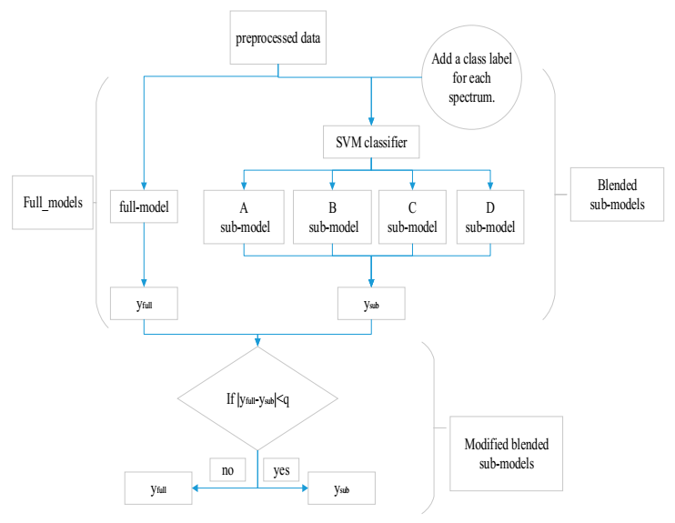
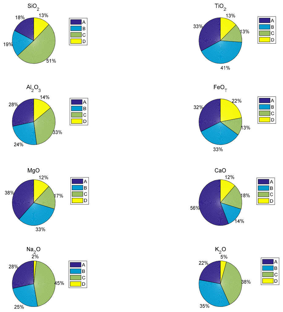
4.1. Selecting a Sub-Model by the SVM Classifier

Before training SVM classifiers, the classes of spectra needed to be defined according to their content of oxides. Spectra in different concentration ranges were put into different groups, and the spectra in the same group belonged to one identical class. For example, the spectra whose contents of silica ranged from 0% to 30% were put into “A” group, and these spectra belonged to “A” class. The four ranges for each oxide were user-defined, and more details are shown in

Table 1. Adding a label of class for each spectrum according to its concentration of each oxide.

	A Class	B Class	C Class	D Class
SiO2	0–30%	30–50%	50–70%	70–100%
TiO2	0–0.5%	0.5–1%	1–2%	2–100%
AL2O3	0–10%	10–15%	15–20%	20–100%
FeOT	0–8%	8–15%	15–20%	20–100%
MgO	0–2%	2–3.5%	3.5–7%	7–100%
CaO	0–2%	2–7%	7–19%	19–100%
Na2O	0–0.5%	0.5–1.9%	1.9–5.4%	5.4–100%
K2O	0–0.6%	0.6–2.7%	2.7–5.3%	5.3–100%

. Figure 3 shows the proportion of samples for each class. Based on the contents of eight major oxides, each oxide was divided into four classes, “A”, “B”, “C”, and “D”. In addition, the presentations of two datasets (D and T) were changed into the following forms (Equations (14) and (15)).

$$D={\{x_i,y_i,z_i\}}_N^{i=1}$$

(14)

$$\mathrm{T}={\{x_i,y_i,z_i\}}_M^{i=1}$$

(15)

where zi is the class of ith spectra. The spectral classifiers were trained on the spectral data (x) and the spectral classes (z) of the training set by using SVM algorithm. The test dataset spectrum were classified in different sub-models by the SVM classifier firstly. Then the corresponding sub-model was used for regression analysis of these spectra.

This section was not mandatory but could be added if there were patents resulting from the work reported in this manuscript.

To train an SVM classifier, two essential parameters (C and γ) needed to be specified, which determined the performance of models. As a key factor for the establishment of the hyperplane, C represented the fault-tolerance. When C was bigger, the tolerance towards errors was low for models, and it was easy to result in a condition called over-fit, which meant the models performed better in the training set while predicting the testing data inaccurately. On the contrary, when C was smaller, the models could not capture enough details of spectra, and this condition was called under-fitting. γ was the vital parameter of the radial basis function (RBF) which mapped the spectra into a higher dimensional linear separable space. The smaller γ was, the higher the number of the support vector was. Furthermore, the number of support vector influenced the speed of the model training. The solution for best choosing the two key parameters was to utilize the method of “3-fold cross-validation (CV)” in the training set. The “3-fold CV” could be described as the spectra in the training set which were divided into three parts: One was used for calibration, while the other two were used for training a model. For eight SVM classifiers, we needed to specify eight sets of parameters by the “3-fold CV”. For each SVM classifier, we firstly set a threshold value (99%) of CV accuracy. When the CV accuracy exceeded the threshold value, the process of parameters’ optimization would be terminated. C and γ under the maximum CV accuracy were chosen as final parameters of SVM classifiers. Then the final parameters were to be used to train SVM classifiers on the whole training set and generate final models.

According to the defined classes of spectra in this paper, the spectra in each class would be used to train a PLSR sub-model, and four PLSR sub-models (A PLSR sub-model, B PLSR sub-model, C PLSR sub-model, and D PLSR sub-model) were needed to be trained for each oxide. PLSR full models were trained on the full composition range in order to compare with sub-models.

4.2. The Optimized Method for Final Outputs of Blended Sub-Models a Sub-Model

The SVM classifiers could not make all spectra exactly find their corresponding sub-models because of misclassification. In order to minimize the errors caused by misclassification, an optimized method for a final output of blended sub-models was utilized in this paper. The optimized process had two steps: Firstly, we calculated the absolute value of the difference between outputs of a full model and a sub-model. Then, if the absolute value was bigger than a user-defined threshold value, the output of the full model would be selected as the final output, otherwise the output of sub-model would be selected as the final output. The equation of the final output is specified as follows (Equation (16)).

$$y_{blended}=\left\{\begin{array}{c}{y}_{full}, |y_{full}-y_{sub}|>=q\\ y_{sub},else\end{array}\right.$$

(16)

where q is a user-defined threshold value, yfull is the output of regression full model, and ysub is the output of regression sub-models. In this experiment, for each oxide, the length of minimum composition range (A, B, C, or D) is chosen as the threshold value (q, 20 for SiO₂, 0.5 for TiO₂, 5 for Al₂O₃, 5 for FeOT, 1.5 for MgO, 2 for CaO, 0.5 for Na₂O, 0.6 for K₂O).

4.3. Model Evaluation

The classification accuracy (CA) for the spectra of the testing set was used to evaluate the performance of the SVM classifiers. The equation is shown in Equation (17).

$$CA=\frac{N_{true}}{N}$$

(17)

where Ntrue is the number of samples with correct classification, and N is the number of all samples.

The root mean square error of predicted concentrations (RMSEP) and R-squared (R²) of the testing set were used as assessment metrics of the regression models. The forms of RMSEP and R² are described in the following equations (Equations (18) and (19)).

$$RMSEP=\sqrt{\frac{{\displaystyle \sum _1^N{(y_{i,actual}-y_{i,predicted})}^2}}{N}}$$

(18)

$$R^2=1-\frac{{\displaystyle \sum _1^N{(y_{i,actual}-y_{i,predicted})}^2}}{{\displaystyle \sum _1^N{(y_{i,actual}-{\widehat{y}}_{actual})}^2}}$$

(19)

where yi, actual is the actual value of ith sample, yi, predicted is the predicted value of ith sample, and actual is the mean value of all actual value.

5. Results

5.1. Performances of Regression Sub-Models and SVM Classifiers

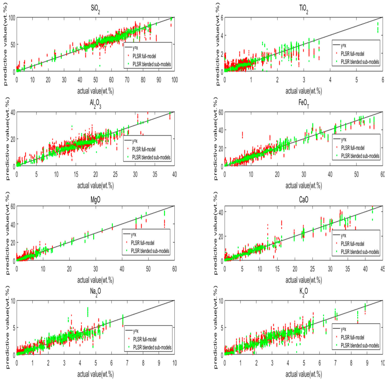
To get the performance of each regression sub-model, a class was also added to each spectrum in the testing set according to its concentration, and then the testing set is divided into four parts, named testing sub-set A, testing sub-set B, testing sub-set C, and testing sub-set D.

Table 2. The performances of PLSR sub-models.

	Sub-Model	Training Spectra	Testing Spectra	RMSEP of Each PLSR Sub-Model
SiO2	A sub-model	600	300	0.9004
	B sub-model	1614	810	0.9227
	C sub-model	4314	2160	1.3831
	D sub-model	959	480	1.0504
TiO2	A sub-model	2200	1100	0.0755
	B sub-model	3240	1620	0.0737
	C sub-model	1074	540	0.1203
	D sub-model	714	360	0.1843
AL2O3	A sub-model	1500	750	0.2758
	B sub-model	1948	980	0.3574
	C sub-model	2760	1380	0.4761
	D sub-model	1260	630	0.6580
FeOT	A sub-model	2080	1040	0.3455
	B sub-model	2680	1340	0.4479
	C sub-model	1294	650	0.4370
	D sub-model	1434	720	0.7856
MgO	A sub-model	2500	1250	0.1240
	B sub-model	2480	1240	0.1469
	C sub-model	1468	739	0.3703
	D sub-model	1000	500	0.6468
CaO	A sub-model	4000	2000	0.1166
	B sub-model	1220	610	0.4008
	C sub-model	1648	830	0.5528
	D sub-model	600	300	1.0975
Na2O	A sub-model	1740	870	0.0833
	B sub-model	1780	890	0.1163
	C sub-model	3608	1810	0.2592
	D sub-model	200	100	0.7203
K2O	A sub-model	1754	880	0.0792
	B sub-model	2514	1260	0.1836
	C sub-model	2620	1309	0.2240
	D sub-model	320	160	0.4929

exhibits the performance (RMSEP) of each sub-model based on PLSR algorithms. For all oxides, PLSR sub-models had lower RMSEPs, which indicated that the performances of sub-models were well. Because each sub-model just needed to predict the concentrations in a narrow, restricted range, the full models had to predict the concentrations in a wider full range. In addition, the RMSEP of each PLSR sub-model was lower than that of each corresponding PLSR sub-model, except for the D sub-model for FeOT and D sub-model for Na₂O.

Table 3. The parameters (c and γ) and performances of SVM classifiers for eight oxides.

	Training Set			Testing Set
	Optimal Parameters of SVM Classifiers		CV	CA
	C	γ
SiO2	97.0059	0.0010	99.6261%	97.8667% (3670/3750)
TiO2	73.5167	0.0030	99.5849%	97.2652% (3521/3620)
AL2O3	48.5029	0.0052	99.2100%	96.6310% (3614/3740)
FeOT	97.0059	0.0017	99.4658%	98.0533% (3677/3750)
MgO	168.8970	0.0017	99.2213%	97.7480% (3646/3730)
CaO	97.0059	0.0010	99.8527%	98.9037% (3699/3740)
Na2O	55.7152	0.0017	99.5497%	97.8474% (3591/3670)
K2O	97.0059	0.0052	99.0844%	96.8975% (3498/3610)
Average	__			97.65%

shows the parameters (C and γ) and classified results of spectra in the testing set. The minimum CA was more than 96.63% for each oxide, and only a few spectra were misclassified. Hence, for eight oxides, the SVM classifiers based on parameters optimized by the 3-fold CV method had better performances in the classification of testing data. The 97.65% of the average correct classification was a satisfactory value and was conductive to select a sub-model. Higher CA meant more spectra could correctly choose the regression sub-models to predict their concentrations.

5.2. PLSR Models

We also constructed PLSR blended sub-models and PLSR full models on the same training set and testing set. The performances of the PLSR blended sub-model and PLSR full model are listed in

Table 4. The performances of 3 various models in the testing set.

Oxide	Training Spectra	Testing Spectra	Modified PLSR Blended Sub-Models	PLSR Blended Sub-Models	PLSR Full Model
SiO2	7488	3750	3.7936	3.1837	5.6280
TiO2	7228	3620	0.4378	0.2309	0.4797
AL2O3	7468	3740	2.0075	1.2711	2.7404
FeOT	7488	3750	2.6758	1.7602	3.5476
MgO	7448	3730	2.1826	0.8550	2.2724
CaO	7468	3740	2.3404	0.9731	2.4510
Na2O	7328	3670	0.7549	0.4948	0.7834
K2O	7208	3610	0.6760	0.4568	0.7009

. For TiO₂, AL₂O₃, FeOT, MgO, and CaO, PLSR blended sub-models achieve lower RMSEPs of 0.2309, 1.2711, 1.7602, 0.8550 and 0.9731, whose RMSEPs fall below 50% from those of the PLSR full models. For SiO₂, Na₂O and K₂O, the RMSEPs of PLSR blended sub-models are 3.1837, 0.4948, and 0.2832 which decrease 30% from those of the PLSR full models. Obviously, PLSR blended sub-models performed much better. Combining these sub-models with SVM classifiers was an effective and novel method for “sub-model” methods, which had a higher academic application prospect.

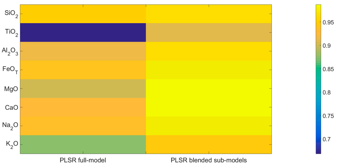
5.3. Effect of Optimized Idea

The final results of the modified PLSR blended sub-model was listed in Table 4. For eight oxides, the RMSEPs of the modified PLSR blended sub-models were much lower than those of PLSR full models. That is to say, compared with PLSR blended sub-models, the modified PLSR blended sub-models was not improved. The reason why the modified PLSR blended sub-models had poor performance may be that during optimization, some spectra classified correctly were treated as misclassified spectra. This phenomenon is called “overcorrection”. Another reason may be that the threshold values of blended sub-models were not the most suitable for PLSR blended sub-models. Although the modified PLSR blended sub-models did not achieve the intended effect, the performance of PLSR blended sub-models was able to prove the efficiency of the new “sub-model” methods, which selected sub-models by classifiers.

5.4. Discussion

In this paper, the regression models with the PLSR algorithm were constructed to demonstrate the performance of selecting a sub-model by a classifier, respectively. Figure 4 shows regression curves between the actual value and the predicted value by PLSR blended models and PLSR full models. The distance of point to the regression line presented the loss of the predicted values. The shorter the distance was, the smaller the loss was, and the more accurate the predicted value was. A temperature map is shown in Figure 5, which exhibited the R² of blended sub-models and full models for eight oxides. R² represented the correlation between the predicted values and the actual values. In the meantime, R² of the PLSR blended sub-models (0.9663, 0.9077, 0.9665, 0.974, 0.985, 0.9873, 0.9727, and 0.9428) were higher than those of the PLSR full models for eight oxides. The higher R2 of blended sub-models illustrated the better performances of blended sub-models than those of full models. The depth of the color indicates the magnitude of the R² value.

For eight oxides, compared with the results of full models, the lower RMSEP and the higher R² of the PLSR blended sub-models strongly confirmed that selecting a sub-model by a classifier was an available idea for the “sub-model” method.

6. Conclusions

In this paper, PLSR models were utilized to prove selecting a sub-model by a classifier is feasible and effective, respectively. The modified PLSR blended sub-models could not only choose sub-models by SVM classifiers, but also improve the accuracy of output, with a 4.3% to 22.7% decrease in RMSEPs compared to PLSR full models RMSEPs. Hence, selecting sub-models by classifiers was a novel and useful approach to the “sub-model” method.

Furthermore, the performance of PLSR sub-model techniques and the conventional PLSR model were also compared in the R² index. The SVM PLS sub-model showed significant improvement in R² for testing the dataset. It could be obtained through experiments that our method is more suitable for the diverse Mars standard datasets. The authors also observed significant improvements on the lower element composition samples. We still need more work to refine and improve the optimized method. In addition, optimizing the compositional range may bring further improvement, which can perfect the method of sub-model selection by classifiers.

References

1. Yang, J.; Li, X.; Lu, H.; Xu, J.; Li, H. An LIBS quantitative analysis method for alloy steel at high temperature based on transfer learning. J. Anal. At. Spectrom. 2018, 33, 1184–1195. [Google Scholar] [CrossRef]
2. Cousin, A.; Sautter, V.; Payré, V.; Forni, O.; Mangold, N.; Gasnault, O.; Le Deit, L.; Johnson, J.; Maurice, S.; Salvatore, M.; et al. Classification of igneous rocks analyzed by ChemCam at Gale crater, Mars. Icarus 2017, 288, 265–283. [Google Scholar] [CrossRef]
3. Roux, C.P.M.; Rakovský, J.; Musset, O.; Monna, F.; Buoncristiani, J.F.; Pellenard, P.; Thomazo, C. In situ Laser Induced Breakdown Spectroscopy as a tool to discriminate volcanic rocks and magmatic series, Iceland. Spectrochim. Acta Part B At. Spectrosc. 2015, 103–104, 63–69. [Google Scholar] [CrossRef]
4. Sautter, V.; Fabre, C.; Forni, O.; Toplis, M.J.; Cousin, A.; Ollila, A.M.; Meslin, P.Y.; Maurice, S.; Wiens, R.C.; Baratoux, D.; et al. Igneous mineralogy at Bradbury Rise: The first ChemCam campaign at Gale crater. J. Geophys. Res. Planets 2014, 119, 30–46. [Google Scholar] [CrossRef] [Green Version]
5. Rossi, M.; Aglio, M.D.; De Giacomo, A.; Gaudiuso, R.; Senesi, G.S.; De Pascale, O.; Capitelli, F.; Nestola, F.; Ghiara, M.R. Multi-methodological investigation of kunzite, hiddenite, alexandrite, elbaite and topaz, based on laser-induced breakdown spectroscopy and conventional analytical techniques for supporting mineralogical characterization. Phys. Chem. Miner. 2014, 41, 127–140. [Google Scholar] [CrossRef]
6. Clegg, S.M.; Wiens, R.C.; Anderson, R.; Forni, O.; Frydenvang, J.; Lasue, J.; Cousin, A.; Payré, V.; Boucher, T.; Dyar, M.D.; et al. Recalibration of the Mars Science Laboratory ChemCam instrument with an expanded geochemical database. Spectrochim. Acta Part B At. Spectrosc. 2017, 129, 64–85. [Google Scholar] [CrossRef]
7. Wiens, R.C.; Maurice, S.; Barraclough, B.; Saccoccio, M.; Barkley, W.C.; Bell, J.F., III; Bender, S.; Bernardin, J.; Blaney, D.; Blank, J.; et al. The ChemCam Instrument Suite on the Mars Science Laboratory (MSL) Rover: Body Unit and Combined System Tests. Space Sci. Rev. 2012, 170, 167–227. [Google Scholar] [CrossRef]
8. Fu, H.; Ni, Z.; Wang, H.; Jia, J.; Dong, F. Accuracy improvement of calibration-free laser-induced breakdown spectoscopy. Plasma Sci. Technol. 2019, 21, 034001. [Google Scholar] [CrossRef]
9. Yang, J.; Li, X.; Xu, J.; Ma, X. A Calibration-Free Laser-Induced Breakdown Spectroscopy (CF-LIBS) Quantitative Analysis Method Based on the Auto-Selection of an Internal Reference Line and Optimized Estimation of Plasma Temperature. Appl. Spectrosc. 2018, 72, 129–140. [Google Scholar] [CrossRef] [PubMed]
10. Lu, C.; Wang, B.; Jiang, X.; Zhang, J.; Niu, K.; Yuan, Y. Detection of K in soil using time-resolved laser-induced breakdown spectroscopy based on convolutional neural networks. Plasma Sci. Technol. 2019, 21, 34014. [Google Scholar] [CrossRef]
11. Guezenoc, J.; Payré, V.; Fabre, C.; Syvilay, D.; Cousin, A.; Gallet-Budynek, A.; Bousquet, B. Variable selection in laser-induced breakdown spectroscopy assisted by multivariate analysis: An alternative to multi-peak fitting. Spectrochim. Acta Part B At. Spectrosc. 2019, 152, 6–13. [Google Scholar] [CrossRef]
12. Anderson, R.B.; Clegg, S.M.; Frydenvang, J.; Wiens, R.C.; McLennan, S.; Morris, R.V.; Ehlmann, B.; Dyar, M.D. Improved accuracy in quantitative laser-induced breakdown spectroscopy using sub-models. Spectrochim. Acta Part B At. Spectrosc. 2017, 129, 49–57. [Google Scholar] [CrossRef]
13. Yuanyuan, C.; Zhibin, W. Quantitative analysis modeling of infrared spectroscopy based on ensemble convolutional neural networks. Chemom. Intell. Lab. Syst. 2018, 181, 1–10. [Google Scholar] [CrossRef]
14. Zhang, X.; Lin, T.; Xu, J.; Luo, X.; Ying, Y. DeepSpectra: An end-to-end deep learning approach for quantitative spectral analysis. Anal. Chim. Acta 2019, 1058, 48–57. [Google Scholar] [CrossRef] [PubMed]
15. Bjerrum, E.J.; Glahder, M.; Skov, T. Data Augmentation of Spectral Data for Convolutional Neural Network (CNN) Based Deep Chemometrics. arXiv 2017, arXiv:1710.01927. [Google Scholar]
16. Padarian, J.; Minasny, B.; McBratney, A.B. Using deep learning to predict soil properties from regional spectral data. Geoderma Reg. 2019, 16, e00198. [Google Scholar] [CrossRef]
17. Fabre, C.; Maurice, S.; Cousin, A.; Wiens, R.C.; Forni, O.; Sautter, V.; Guillaume, D. Onboard calibration igneous targets for the Mars Science Laboratory Curiosity rover and the Chemistry Camera laser induced breakdown spectroscopy instrument. Spectrochim. Acta Part B At. Spectrosc. 2011, 66, 280–289. [Google Scholar] [CrossRef]
18. Boser, E.; Guyon, M.; Vapnik, V.N. A Training Algorithm for Optimal Margin Classifiers. In Proceedings of the 5th Annual Workshop on Computational Learning Theory (COLT’ 92), Pittsburgh, PA, USA, 27–29 July 1992; pp. 144–152. [Google Scholar]
Figure 1. Box plots of concentration distribution for eight oxides. Maximum whisker length is 1.5. Black rhombic points are outliers.
Symmetry 13 00319 g001
Figure 2. Flowchart of the experimental design. Support vector machine (SVM) classifiers and partial least squares regression (PLSR) sub-models were implemented on the MATLAB R2016a.
Symmetry 13 00319 g002
Figure 3. Pie charts show the proportion of samples in each class.
Symmetry 13 00319 g003
Figure 4. The regression curves between the actual value and the predicted value by the PLSR blended models and PLSR full models.
Symmetry 13 00319 g004
Figure 5. R2 of PLSR full models and the modified PLSR blended sub-models for SiO2, TiO2, Al2O3, FeOT, MgO, CaO, Na2O, and K2O.
Symmetry 13 00319 g005