Abstract
Many man-made or natural objects are composed of symmetric parts and possess symmetric physical behavior. Although its shape can exactly follow a symmetry in the designing or modeling stage, its discretized mesh in the analysis stage may be asymmetric because generating a mesh exactly following the symmetry is usually costly. As a consequence, the expected symmetric physical behavior may not be faithfully reproduced due to the asymmetry of the mesh. To solve this problem, we propose to optimize the material parameters of the mesh for static and kinematic symmetry behavior. Specifically, under the situation of static equilibrium, Young’s modulus is properly scaled so that a symmetric force field leads to symmetric displacement. For kinematics, the mass is optimized to reproduce symmetric acceleration under a symmetric force field. To efficiently measure the deviation from symmetry, we formulate a linear operator whose kernel contains all the symmetric vector fields, which helps to characterize the asymmetry error via a simple norm. To make the resulting material suitable for the general situation, the symmetric training force fields are derived from modal analysis in the above kernel space. Results show that our optimized material significantly reduces the asymmetric error on an asymmetric mesh in both static and dynamic simulations.
1. Introduction
Symmetry is a ubiquitous phenomenon in nature and a very essential rule for artistic design. Mathematically, it encodes some invariance of given structures under certain transformations. In practice, symmetry reflects both aesthetics considerations and functionality purposes. Because of its importance, symmetry has been widely used in many geometry processing procedures, such as remeshing, editing, repairing, etc, as well as the virtual reproduction of animations with symmetry for visual realism and artistic harmony.
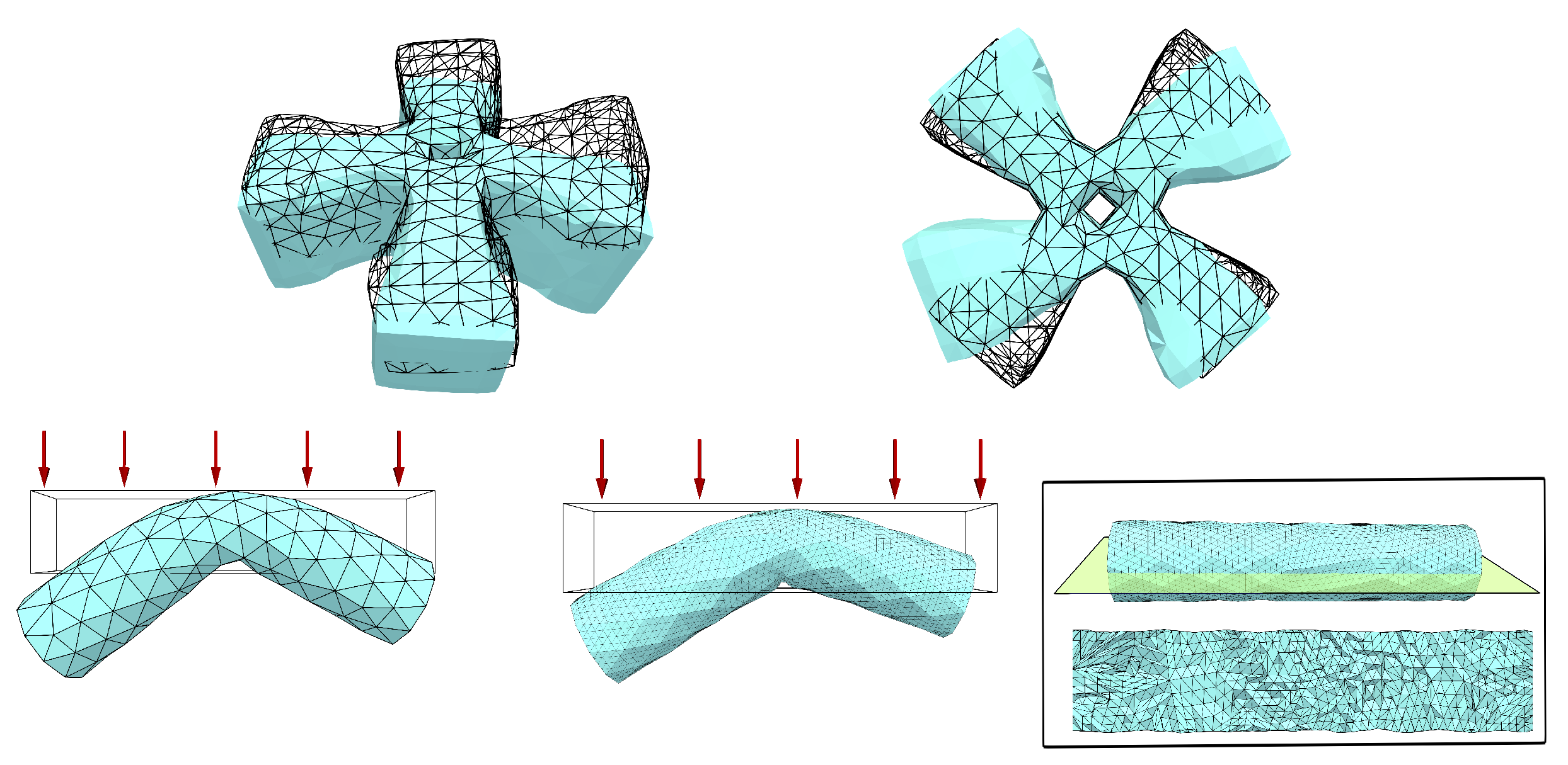
However, at the stage of simulation, the symmetry may be lost. Some models used in computer animation come from 3D scanning or other geometry modeling software. On the one hand, limited by data acquiring techniques and real-world noises, the symmetry of a shape may be broken when transformed into digital representations. More importantly, even if the shape is in perfect symmetry, e.g., modeled by software, the mesh tessellated from the shape could be asymmetric. The elastic simulation based on the asymmetric mesh may result in asymmetric behavior. In other words, the displacement or acceleration may be not symmetric even if the force field is in symmetry (see Figure 1). To reduce the asymmetric artifacts, increasing the mesh density may help, but the additional computational cost is not affordable in some real-time applications (e.g., game, virtual reality). If the mesh has some asymmetrically distributed badly shaped elements, which brings strong shear locking, we also notice that refining the mesh by subdivision cannot easily reduce the asymmetrical behavior (see Figure 1).

Figure 1.
Asymmetric deformations caused by meshing. Even subdividing the meshes, asymmetry still exists, which is largely due to the asymmetrically distribution of badly shaped elements as shown in the close-up figure of the cut section.
To get rid of such undesired asymmetry artifacts, a natural idea is to generate a symmetric mesh, and a few works (e.g., [1]) do make such attempts. However, they are not generally applied and cannot be used for generating the desired volumetric meshes. It is worth noticing that it is even impossible to generate meshes with the desired symmetry sometimes. For instance, no structural hexahedral mesh can have the correct symmetry at the rotational axis of a fan with five symmetric blades.
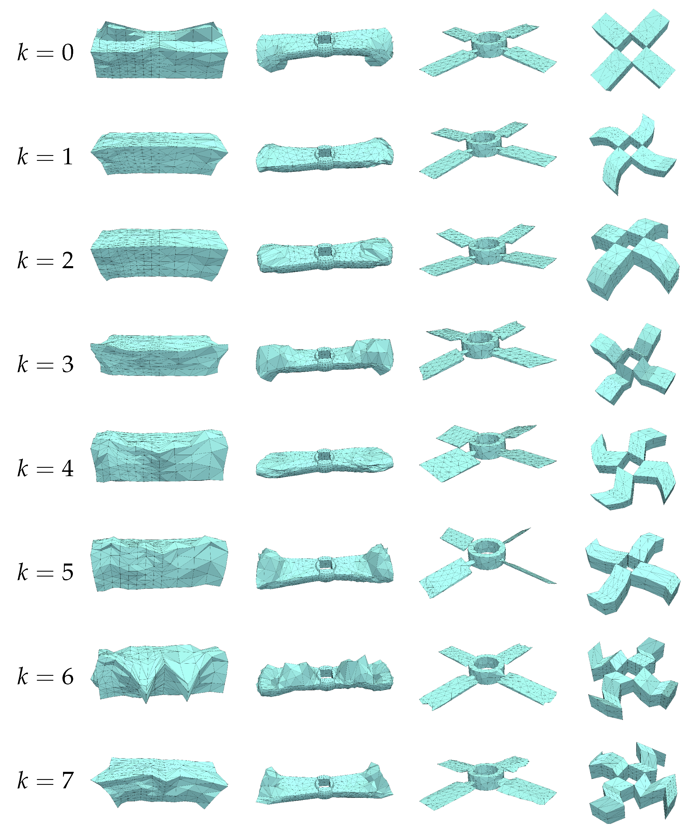
There are other possible remedies. One can impose constraints or use post-processing to modulate the elastic simulation so that the displacement or even acceleration is symmetric. However, such a way introduces artificial ingredients into the simulation, and the constraints or the post-processing are not easy to design for general situations. Roughly speaking, such a way is very restricted and not applicable in general elastic simulation involving asymmetric boundary conditions. A more flexible method is to refine the mesh or use a high order basis function to reduce the impact of asymmetry in the mesh. This strategy results in a larger or denser system matrix, and the additional cost may not be affordable for some applications that require intensive user interactions and rapid feedbacks.
Considering the above-mentioned issues, we instead propose to optimize the material to compensate the error coming from asymmetric meshes. Unlike refinement approaches, our method keeps the problem size and matrix sparsity. Consequently, numerical performance will not be notably affected while desired symmetry behaviors can be nicely preserved with the optimized materials. Moreover, once the material gets adjusted, it can be generalized to solve a series of problems defined over this object without any necessities for specifically designed constraints or post-processing, thus saving enormous cost on computational or operational efforts and allowing for better interactivity for editing or design tasks.
Technically, there are two challenges to be addressed. Firstly, a clear mathematical definition of symmetric behavior is required. Secondly, a reasonable symmetry-deviation measurement is necessary—because even if the material gets optimized, it is generally not possible to have symmetric behavior in any case. To address these two challenges, we make the following contributions:
- Both static and kinematic symmetry behaviors are considered. Under a symmetric force field, we ask the displacement of the static equilibrium status and acceleration in kinematic simulation to be symmetry.
- We find that all the above symmetric vector fields fall in the kernel of a linear operator associated with the symmetry. Therefore, the asymmetric error can be efficiently measured via a simple norm.
- Taking the common assumption used in modal analysis that low frequency modes dominant the behavior, we formulate the physical equation in the above kernel space and take its leading eigenvectors as the training force fields so that the resulting material can be generally applied.
To justify the proposed method, we show results on various meshes with rotational and mirror shape symmetries, as well as an illustration on symmetric behavior in dynamic elastic simulation. The asymmetric error generally deceases greatly after using an optimized material, which clearly shows the benefits of our method.
2. Related Work
2.1. Symmetry
Symmetry analysis and its application have been an active area of research for a very long time. Many works have been proposed to detect or use symmetry in geometry processing. A detailed survey in this area can be found in [2]. Here, we only mention some of the works that are closely related to ours.
For symmetry detection, different methods have been proposed to handle different kinds of symmetries. Early methods can only detect global symmetries [3] for the whole model, while most recent ones could find partial symmetries. Podolak et al. [4] extracted approximate and partial reflection symmetries. Mitra et al. [5] and Shi et al. [6] covered symmetries under similar transformations. In our work, we use the method of Lie algebra voting proposed in [6] to detect symmetries.
For symmetry-aware applications, most of the previous works focused on geometry processing. Dessein et al. [7] used symmetry to tessellate the input mesh into symmetric patches. Thrun et al. [8] reconstructed a complete model from partial 3D views by considering symmetry relations. Wang et al. [9] proposed a high level structural representation of a 3D model by grouping parts using symmetry or connectivity. Chen et al. [10] incorporated symmetry information into the parametric model of the 3D human body. However, to the best of our knowledge, we have not seen any work considering symmetry in physically based simulation.
2.2. Material Optimization
FEM-based deformable object simulation is a well-studied topic in graphics-related community. A through review of the methods can be found in [11,12] and the references therein. In simulation, the material plays an important role that governs the physical behavior of the deformable objects. Our method optimizes the material, specifically Young’s modulus in each element; therefore, it naturally relates to many material optimization methods, though aiming at a different purpose.
Material optimization is often used in physical property related modeling [13,14,15] and its downstream applications of computational fabrication (e.g., 3D printing) [16] and topology optimization via homogenization [17], etc. Many methods “reconstruct” the material by optimization to fit the measurement from the real objects with data acquisition devices [13,16,18,19,20]. There are also methods to “model” the material with respect to a certain designed goal. For instance, Xu et al. [14] explicitly optimized the material parameters to make the object reach a specific shape under a specific force. The mathematical model of a material, i.e., the “parameters” to describe the material, plays an important role in such research. Xu et al. [21] provided an explicit nonlinear material model via the principal stretches of the material. Miguel et al. [22] proposed a method for a hyperelasticity material. The model of the material and the specific numeral method are different in those methods, but they generally take pairs of the force field and the associated displacement field as the input. Sharply different from them, there is no pair of force and displacement fields in our method. When the force field is symmetric, we just ask the displacement field to satisfy the symmetric condition, but we do not need to specify a target field.
In material optimization, the problem is usually highly non-linear, which brings many challenges for numerical solving. Many techniques are proposed to address such issues. For efficiency, some methods rely on the reduction of the solution space [14,15,19], while some others apply Sherman–Morrison–Woodbury formulas for fast inverse computation [23]. Recently, Yan et al. [24] improved the efficiency by alternating between two phases, forward simulation and parameter updating in an inexact descent manner. Because the error coming from the asymmetric mesh is usually distributed in a non-smooth way, the adjustment of the material to compensate such error is often non-smoothly distributed. As a consequence, the former technique [14], i.e., solving the problem in a solution space spanned by a few smooth bases, is not applicable. The latter one [23] makes an assumption that the correction of the stiffness matrix is in low rank, which does not hold in our case. Therefore, we roughly follow the method in [14] to solve the problem, but do not apply reduction.
3. Symmetry Behavior
In this section, we briefly introduce the notion of shape symmetry for a deformable model. Based on that, we treat the symmetry of the displacement, acceleration, and force fields in a similar way, by means of unifying them as a symmetric vector field attached to the model. Finally, we integrate the symmetric fields into the elastic model to characterize the expected symmetric behavior.
3.1. Shape-Symmetry
First of all, we need to define precisely what the symmetry of a shape is before any discussion. Mathematically, symmetry implies a kind of invariance under the actions of a group of transformations. Here, let us investigate a 3D model , i.e., a subset in 3D vector space associated with the standard Euclidean metric. We say that is symmetric under transformation if and only if [2]. The symmetry transformation g can be manually specified or automatically detected via algorithms [5,6]. We only consider isometric transformation g in this work, which can be encoded by a combination of rotation (or reflection) part T and translation part t: . By definition, any point has its counterpart .
3.2. Symmetry of Fields
We first discuss the symmetric behavior under the static equilibrium state. To be more specific, the model should be deformed into a symmetric shape under a static equilibrium state when the symmetric force field is applied. Mathematically, for a model with symmetry g, when applying a force field with the same symmetry g, the resulting displacement field should be symmetric with respect to g as well. In other words, a symmetric point pair keeps symmetry when it moves to new positions :
or equivalently (by ):
thus, we have:
The symmetry of the force field can be described similarly because it can be viewed as an offset vector field directly added to the rest state, but later, it will be transformed into “real” displacement by the elastic model. In this sense, a force filed is symmetric if it satisfies the following equation similar to Equation (3):
To sum up, the symmetry of both the displacement and force fields can be characterized by the same equation. Given a vector field z expected to be symmetric under g, we can define the deviation from the symmetry at as:
where the anti-symmetric part of z, i.e., , is linear to z via a linear operator S. The overall deviation of symmetry for z can be measured via the norm energy of , i.e.,
For the sake of efficiency, the above measurement of asymmetry can be evaluated on a pair of subsets associated with symmetry g, i.e., . Comparing with Equation (6), the resulting measurement:
is only evaluated on part of the model and can save the computational cost of generating training force fields, which will be explained later. We interactively construct such symmetric subsets in our implementation, but automatic methods with previous symmetric segmentation techniques [5,7,25] are also available. As an illustration, we enclose and for the CAD model in Figure 2. Here, and follow the mirror symmetry associated with the reflection T, and the symmetric force field on them should also obey the symmetry, i.e., .

Figure 2.
Symmetric force field and symmetric subsets.
Such a subset based formulation also helps for models with multiple symmetries. The left fan model in Figure 2 has four blades with the same shape, but different orientations. There are indeed several symmetries, e.g., , , and rotations denoted as respectively. Taking one blade as , each rotation is associated with another blade . Applying Equation (7) to with measures the asymmetry for vector field z on these two blades, which leads to a linear operator defined on . To measure the deviation of symmetry on the whole model, we simply sum all three measurements associated with , which boils down to the linear operator that characterizes these symmetries on the fan model.
3.3. Symmetric Behavior
The displacement field, or its dynamic evolution, is a response from the object’s physical model to the applied external force field. We will revisit the problem of computing static equilibrium and dynamics and explain how our idea is applied then.
In the common linear elasticity model, the equation of motion relates the acceleration, displacement, and force via:
where is the acceleration. M is the mass matrix, and the stiffness matrix is the Hessian of the potential energy being quadratic in u.
To measure how the physical behavior is symmetric, except for the symmetric force field f, we also apply symmetric position constraints, i.e., fixing some symmetric point pairs:
The specific choice of point set depends on the application. As an illustration, the fixed points are marked with a red sphere in Figure 2. More examples can be found in Section 5. In our implementation, we approximate these constraints via mass-springs, which brings the following additional potential energy:
which augments the total potential energy into and Equation (8) is thus turned into:
where . Taking the widely used implicit integrator [26] in the simulation, the above equation results in the following equation with time step size h for acceleration a:
where are the displacement and velocity at the beginning of this time step.
For simplicity, we start from the symmetric behavior at static equilibrium status, i.e., the status when acceleration and velocity ; thus, the above equation can be simplified into:
Naturally, the displacement u should be symmetric under symmetric force field f. It is easy to see that characterizes the linear relationship between u and f, where is related to the material.
Our idea is to properly scale at each point with a scalar field by minimizing the symmetric deviation energy according to Equation (7). Scaling is equivalent to scaling Young’s modulus because the local stiffness is linear to the local Young’s modulus. The lower and upper bounds, denoted by and , respectively, are user specified parameters to constrain the range of scaling factors. It is well known that the common displacement formulation in the finite element method is generally over stiff due to insufficient degrees of freedom. Therefore, there is not much sense to further increase Young’s modulus when optimizing the material. Thus, we experimentally set and as and one, respectively, to prevent the material from stiffening. Similar to many material optimization techniques, we also regularize s by asking it to be close to one:
As for the dynamics, the acceleration field a in Equation (11) is expected to be symmetric at rest status when f is symmetric. According to Equation (12), we have:
(i.e., Young’s modulus) should not be changed here, otherwise the symmetric behavior may be lost at static equilibrium status. The mass M encoding the inertia also plays a crucial role in determining the kinematic behavior and will be optimized. The approach for optimizing can be similarly applied here. A scalar field is used to compensate the asymmetric mass distribution caused by asymmetric tessellation. The regularization on r has the same form in Equation (14).
For the sake of simplicity, we will explain our method mainly based on solving symmetric equilibrium states in the following sections.
3.4. Training Force Fields
In practice, it is difficult to obtain a scale s that makes the resulting displacement field u satisfy for arbitrary symmetry force field acting on and . Therefore, we sample a set of force fields and solve the following optimization,
where is set to experimentally. Following Equations (7) and (13),
measures the deviation from the symmetry for training forces , and weights the asymmetric error associated with training force . The training forces and their weights are carefully selected following the overall idea of modal analysis, but are restricted in the linear subspace . Roughly speaking, we want to obtain symmetric force field minimizing the energy under the constraint that they should be orthogonal to each other:
is indeed the eigenvalue in the linear subspace for . Its inverse naturally assigns large weight for low frequency modes in the deviation of the symmetry. This heuristic weighting scheme relaxes the error penalty for non-smooth high frequency modes and manages to better keep the symmetry for smooth low frequency modes, which dominants the common behavior.
4. Discretization and Numerical Method
In this section, we show our implementation for the above formulations. We show how to apply the aforementioned method to an model discretized by a tetrahedral mesh composed of a node set and an element set with piece-wise linear shape functions. Other discretization strategies, such as higher order FEM or even meshless methods, are also feasible.
To discretize the key equation Equation (7), some points in are sampled, and the integration is approximated by the weighted sum of . To be specific, the sampling points are the boundary nodes of in , i.e., . The weight for each sampling point is the area of the Voronoi cell in . It should be noticed that we indeed just evaluate the integration on the boundary of the mesh, but it works well in our experiments. The set contains all the points symmetric to . If happens to fall outside of , we use its nearest point on to replace it.
Denoting the flattened vectors of all nodal coordinates in , and as , , and , respectively, we can have two sparse matrices to interpolate the positions of the points, i.e., and . The symmetry of these two point sets can be verified by:
where and . The linear operator in Equation (7) is then discretized as a matrix:
Following the common linear FEM strategy, a 3D vector field z, which can be a displacement field u, acceleration field a, or a force field f, is encoded on each node and linearly interpolated in each element, and thus can be represented as . The vectors on the above points can be interpolated by . As a consequence, the integration in Equation (7) can be approximated as:
where is a diagonal matrix whose entries are the aforementioned weight for each sampling point.
The discretization of the elastic model and other parts is in the common way. The scale of Young’s modulus s is piece-wise constant in each element, and thus can be represented as a vector . The global stiffness matrix is assembled from local stiffness matrices computed on each tetrahedral element. Because scaling Young’s modulus of the original material is equivalent to scaling the local stiffness matrix, we have:
where is the scale in the e-th element. The stiffness matrix for element e is pre-computed with the input Young’s modulus. The scale of mass is encoded on each node, thus represented as a vector as well. We use the lumped mass matrix, and the entries related to the n-th node in this diagonal matrix have the value where stands for the input mass of this node. The energy to fix symmetric points is simply reduced to:
where is a sparse matrix to interpolate the displacement of and from . The stiffness matrix for these constraints is .
Putting all of them together, Equation (11) becomes a linear system in dimensions:
The training force field is in the kernel of . Moreover, those forces of the nodes that are not involved by are all , which intuitively means that we do not apply any force on such nodes not in and or algebraically meaning that if the column of is all zeros, then the corresponding component of is zero. Actually, we are more interested in some symmetric forces, which implies that this force is in the kernel space of S. A set of bases for can be extracted by singular value decomposition of . Given a matrix with columns composed of such bases, we solve the following general eigenvalue problem for associated with non-trivial eigenvalues:
is similar to , but composed of the Voronoi volume for every node in . The training force fields simply become , where are the columns of . For better understanding, We visualize the shape of the training forces of different models in Section 5.3. The weight of asymmetric measurement for is , and the number of forces N is set to 40 experimentally in all of our experiments. One can set as or as , but this will significantly increase the computational cost of the singular value decomposition here.
The asymmetric energy term F in Equation (17) is thus discretized as:
and the regularization term is:
where is an diagonal matrix with entries being the volume of the i-th element in mesh , and here is a constant -D vector whose entries are all ones.
Finally, the optimization problem becomes:
Note that when we are further attempting to symmetrize kinematic behavior, the objective function can be thus replaced by:
in conjunction with the additional regularization term and box constraints on variable . There is no need to alternatively optimize the stiffness scaling and mass scaling , because they are indeed decoupled and used to symmetrize the static equilibrium and kinematic behavior, respectively. The stiffness scaling can be simply fixed after getting optimized in the equilibrium step for efficiency, which is also helpful to keep an invariant static equilibrium state as the object finally stops moving after a long time.
In addition, some user-controlled parameters are summarized here: , and h are set to , , 1, and , respectively.
Numerical Method
Because the material to compensate the asymmetric mesh is not smoothly changed in the general situation, existing acceleration techniques like dimension reduction [14] are not applicable. Instead, we solve the material optimization problem in full space.
The Hessian of the objective function in Equation (28) is a dense matrix, which leads to very high computational cost by the common Newton method. Therefore, we take the L-BFGS method provided by the ALGLIB library [27] with box constraints because it just needs the gradient of the objective function derived in Appendix A. During the optimization, we set as the initial guess and take a simple diagonal preconditioner provided in Appendix B to accelerate the convergence. We use multiple conditions for termination: if one of the following conditions satisfies, i.e., the change of the objective value, or the change of the step value, , or the norm of the gradient, is less than the corresponding threshold, or the number of iterations reaches the maximum, the iteration stops. In practice, The first three thresholds , , and are set to , and the maximal iteration number is set to 500 in all of our experiments.
5. Results
Unless otherwise specified, we use default parameters mentioned in the last section in the optimization process for all of the following experiments.
5.1. Optimized Symmetric Deformation
In this section, we present side-by-side comparisons of the deformations before and after material optimization on models with reflectional or rotational symmetry.
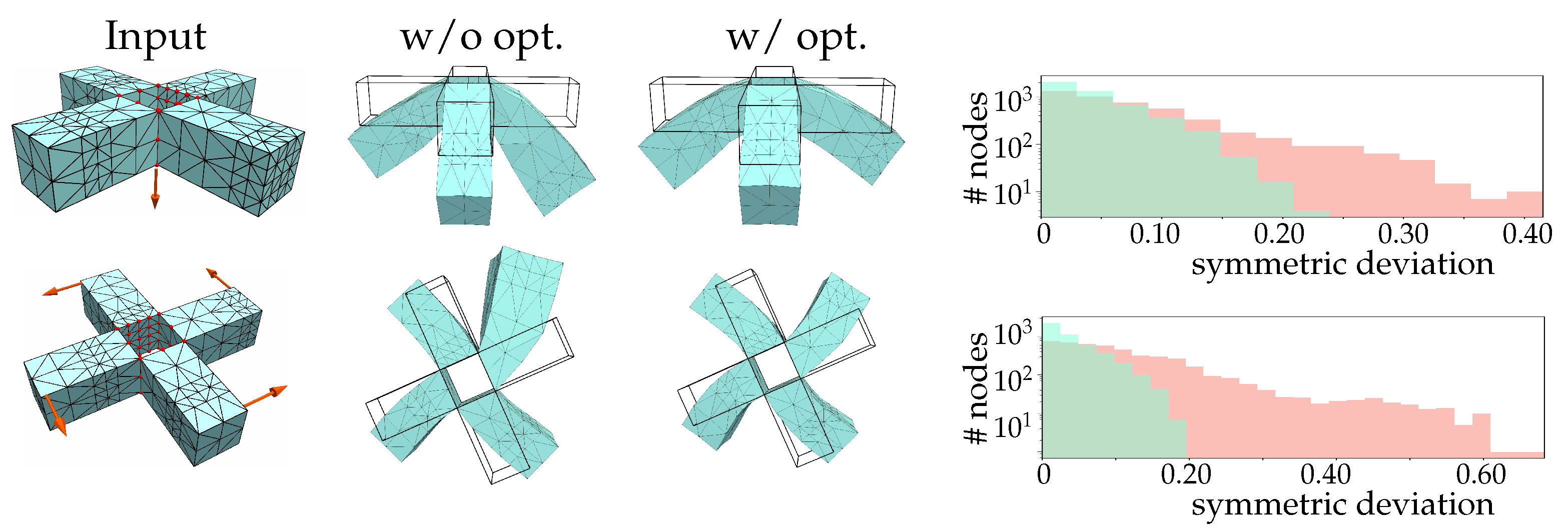
In Figure 3, for a cuboid model, we take points on its reflection plane as fixed and apply the same forces on its two ends (as illustrated in the first row). In the first column, the deformations before and after optimization are presented when the same downward forces are applied on both ends. It is clear to see that the deformation result after optimization becomes more symmetric. The effectiveness of the optimization is also shown in the second row when the outward forces are imposed. Furthermore, the histogram in Figure 3 for the distribution of the symmetry error on all the nodes clearly demonstrates the effectiveness.

Figure 3.
Deformation of a cuboid model under different forces. We use a linear material with Poisson’s ratio and Young’s modulus . The top and bottom rows show the deformation results under a downward and an outward force, respectively. In both cases, points on the reflection plane are fixed. In the middle columns, we show the deformation result before optimization (w/o opt.) and after optimization (w/ opt.). As for a quantitative evaluation, we also calculate the symmetry deviation per node. After optimization (green), the error distribution among nodes is significantly refined compared to its unoptimized counterpart (red). Before optimization, the averaged nodal symmetric deviation is for the first example and for the second. After optimization, this metric reduces to and , respectively.
Similar results can be obtained for models with rotational symmetry. The cross model in Figure 4 has four symmetric parts. Just like the fan model in Figure 2, it has three multiple rotational symmetries. We fix points on the innermost layer (as shown by the red points in the first row) and illustrate its deformation results under two symmetric forces before/after optimization. As is shown in the figure, the deformations under the downward or the spin force after optimization are much more symmetric than those before optimization as well.
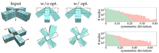
Figure 4.
Deformation of a cross model under different forces. We still use a linear material with Poisson’s ratio and Young’s modulus . The top and bottom rows show the deformation results under a downward force and a spin force, respectively. In both cases, points on the innermost layer are fixed (red points in the first column). The histograms count the same metric as Figure 3. Before and after optimization, the first deformation example has an averaged nodal symmetry deviation of and , respectively, while they become and for the second example.
It is worth noticing that although being simple in geometry, these two examples clearly show the benefits of our material adaption regarding the deformation symmetry. For ever more complex models, things could get even worse, where neither discrete shapes nor the tessellations can easily stay perfectly symmetric in the discretization. A rough, irregularly sampled, or even non-manifold input surface mesh could seriously destroy the regularity of the resulting volumetric meshes, further making the solutions on the generated meshes look hardly close to symmetric, while our method notably overcomes existing defects in meshing.
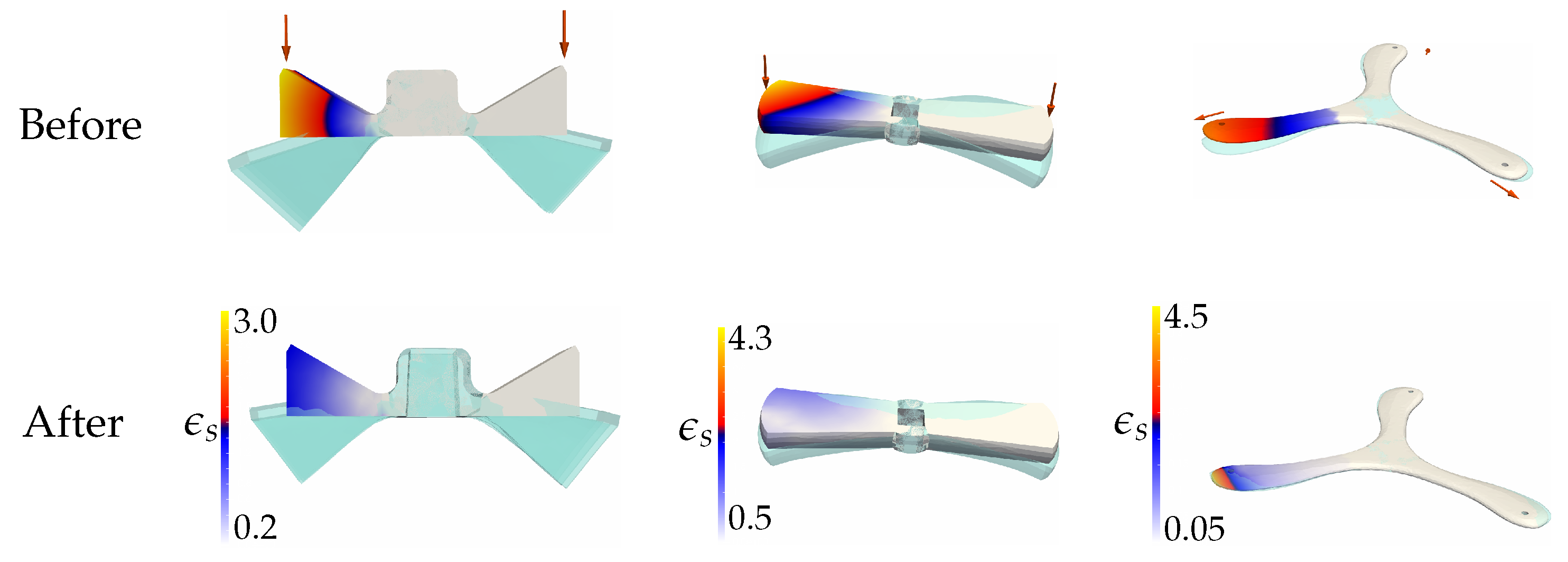
Furthermore, to conduct quantitative assessment on the results, we also show the symmetric displacement error on each sampling point in one of the symmetric parts (e.g., in Equation (7)). The symmetric displacement error on a sampling point is defined as:
In Figure 5, we compare both the deformation results and the distribution of on a few models before/after optimization. In this figure, all symmetric forces are applied on the ends of models with the center part of the models being fixed. In such a setting, sampling points near the end of the model generally have larger symmetric displacement error. As for the symmetric displacement error , it tends to be smaller after optimization, which leads to a better deformation result (more symmetric).
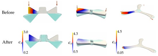
Figure 5.
Visualization of the distribution of symmetric displacement error on sampling points in one of the symmetric parts (other parts are shown in white color). The color bar of is shown for each model. The value increases as the color varies from blue to red. For all these models, symmetric forces applied to their ends with center parts are fixed.
5.2. Optimized Material Distribution
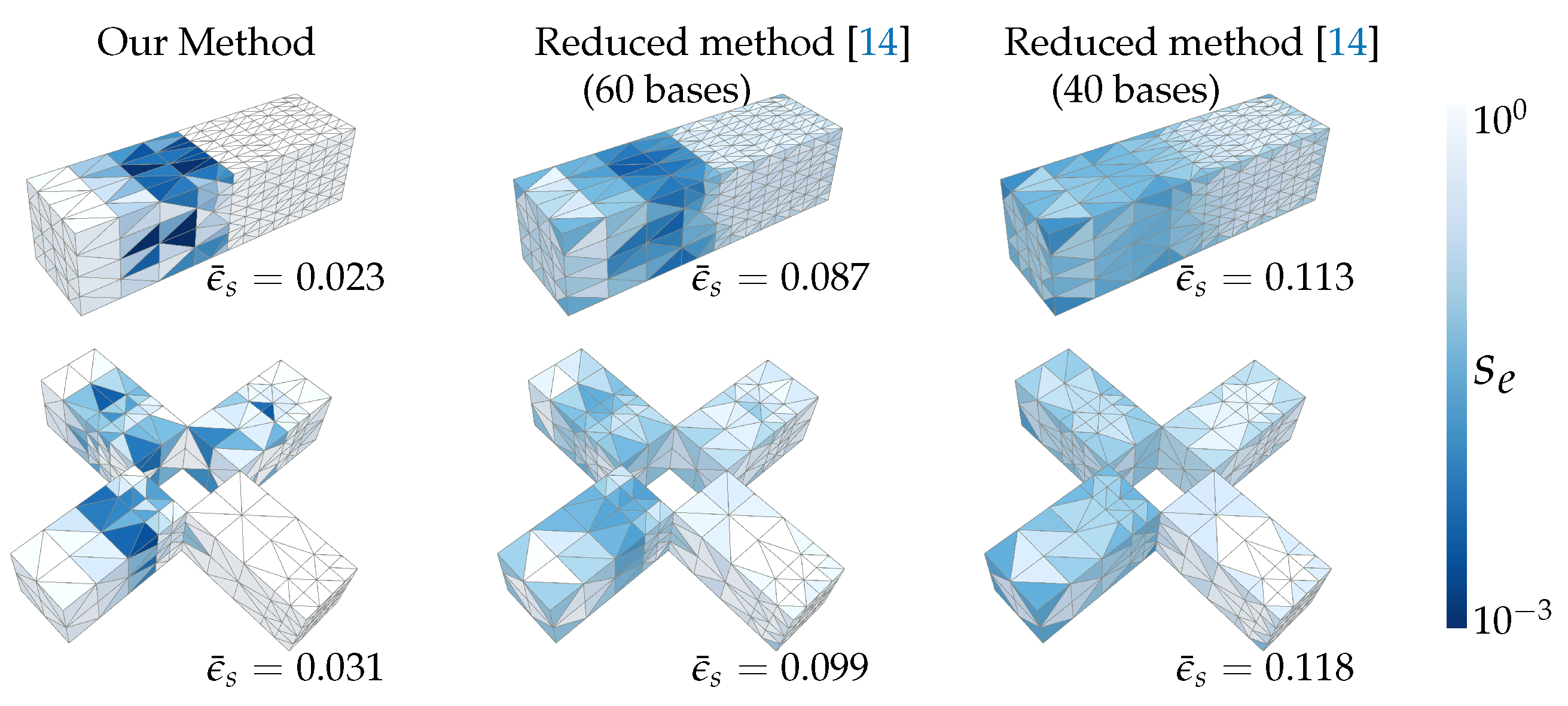
In this section, we look into the optimized material. The optimized material can be represented by the stiffness scale on each element. In Figure 6, we visualize the scale field on the cuboid model (Figure 3) and the cross model (Figure 4). Note that these two models have very different tessellations in the symmetric parts. It can be observed that, in the symmetric parts, big elements tend to have a small stiffness scale, which could compensate the numerical stiffness. On the contrary, small elements tend to have a large stiffness scale, making them more stiff. Overall, the optimized material makes the deformation result symmetric under symmetric forces, as was illustrated in the previous section.
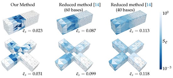
Figure 6.
This figure shows the optimized material for the cuboid model (left) and the cross model (right) by visualizing the stiffness scale on each element. Generally, big elements have a small stiffness scale to compensate their numerical stiffness and vice versa. Compared to applying the reduced method [14] to optimize the material, although being faster in the computations, the resulting material could be undesirably smoothed out and introduce a large error. In this figure, the error is computed as . These two examples have an average nodal symmetry deviation of 0.245 and 0.259, respectively, without material optimization.
Most of our previous experiments fix points near the reflection plane or rotation axis of a model, which is common in practice. However, our method does apply to other scenarios as well. For example, for the cuboid model, we can also fix points on its ends and apply symmetric forces to the other part of the model. As shown in Figure 7, the sampling points on the end of the cuboid (red sphere in (a)) are fixed, while downward force is applied to the whole model. In this case, the deformation result after material optimization also becomes more symmetric. From the comparison results of Figure 6 and Figure 7, we can see that different fixed points lead to a different optimized material. This implies that the material optimized for one boundary condition may not be suitable for others. As a limitation, this will be discussed at the end of this paper.

Figure 7.
Another setting of fixed points for the cuboid model. In this experiment, the sampling points colored in red on the end of the model are fixed (a), and the optimized material is shown in (b). We use a linear material with Poisson’s ratio and Young’s modulus . In this case, we apply a downward force to the whole model, and the result shows that after optimization (d), the deformation result is also more symmetric than before (c).
5.3. Kernel Forces Visualization
To make it easy and intuitive to understand the force at different modes, we visualize some of these modes in Figure 8.
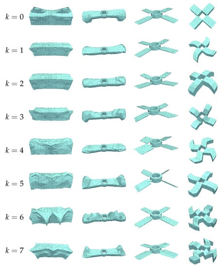
Figure 8.
Visualization of the first eight kernel vectors of (i.e., the training forces). The kernel vectors associated with smaller eigenvalues are smoother and dominate the physical behavior.
5.4. Performance
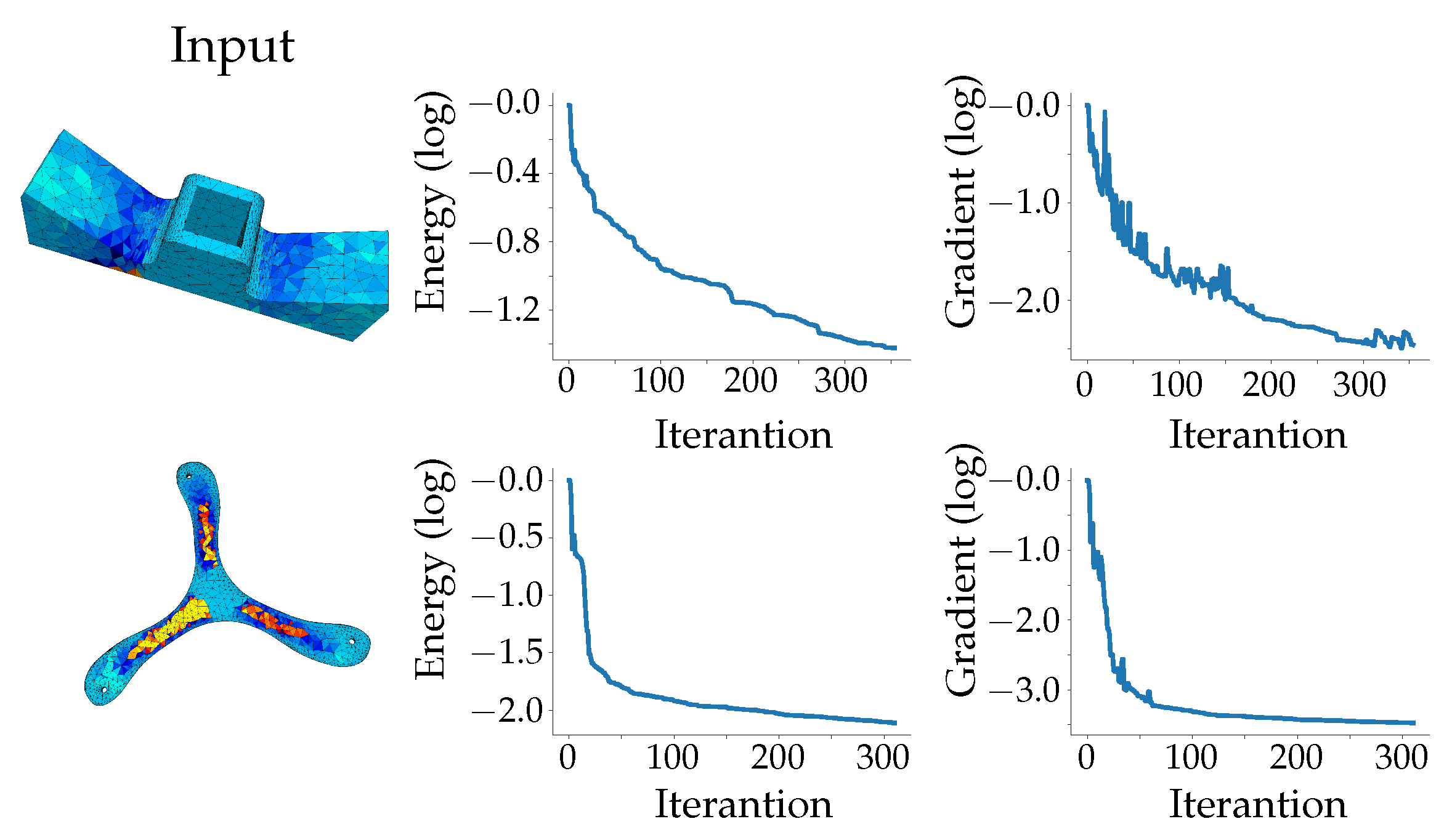
The performance of our algorithm is investigated in this section. In all of our experiments, the optimization energy in Equation (28) drops quickly in the first few iterations and mostly converges in less than 350 iterations, as is shown in Figure 9.
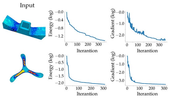
Figure 9.
Statistic of the energy value and gradient (Frobenius norm) for the material optimization of two models. In the curve graph, the energy values and gradient norms are normalized by their initial values and taken by the logarithm, so that the magnitude change of their values could be better observed. For both models, the energy values quickly drop in a few iterations.
We also count and analyze the time consumption of our algorithm. In our implementation, there are two time-consuming stages: one is the generation of the training force , and the other is the numerical optimization (Equation (28)). Suppose that one is able to know what kinds of symmetric forces are mostly used in practice, then the optimization can only focus on the forces of interests, which saves the time-consuming effect of computing many kernel vectors in the symmetry subspace. We show the statistic results in Table 1. These results were evaluated on a PC with an Intel®Core™i5-6300HQ CPU @ 2.30 GHz × 4, and 8 G memory.

Table 1.
The time statistics of the material optimization for more models. The second and third rows show the number of vertices and elements , respectively. Constraint num is the number of symmetry constraints. Kernel dim is the dimension of the kernel of . Training records the time of generating , which includes the cost of computing the kernel of and solving the general eigenvalue problem in Equation (25). Optimization records the time of the numerical optimization in Equation (28). The last row displays the total running time of our implementation.
Although such a precomputation step is inefficient, extra cost can be saved in the following stages of numerical optimization. This reveals the fact that our method for symmetrizing solutions does not need to have sharply increasing cost due to mesh or basis refinement. Thus, it is particularly useful to process batches of tasks, e.g., generating a many-frame animation of nonlinear dynamics, as we will show in the next subsection.
5.5. Symmetrizing Dynamics
As mentioned, our idea to adjust the material is not only applicable to elastic stiffness for pursuing symmetric equilibrium statics, but is also able to symmetrize the dynamics by incorporating mass compensation. Once the mass and stiffness have been optimized, the physical model can be applied to simulate a sequence of symmetry-preserving animations without the need for frame-by-frame manual editing. In this subsection, we show that our method provides a preliminary method for the dynamics simulation. Indeed, our method just “symmetrizes” the dynamic behavior around the rest state. Integrating the co-rotational method, we can achieve some natural results under large deformation. However, general non-linear elastic models will bring big challenge to our method, which is reserved for future exploration.
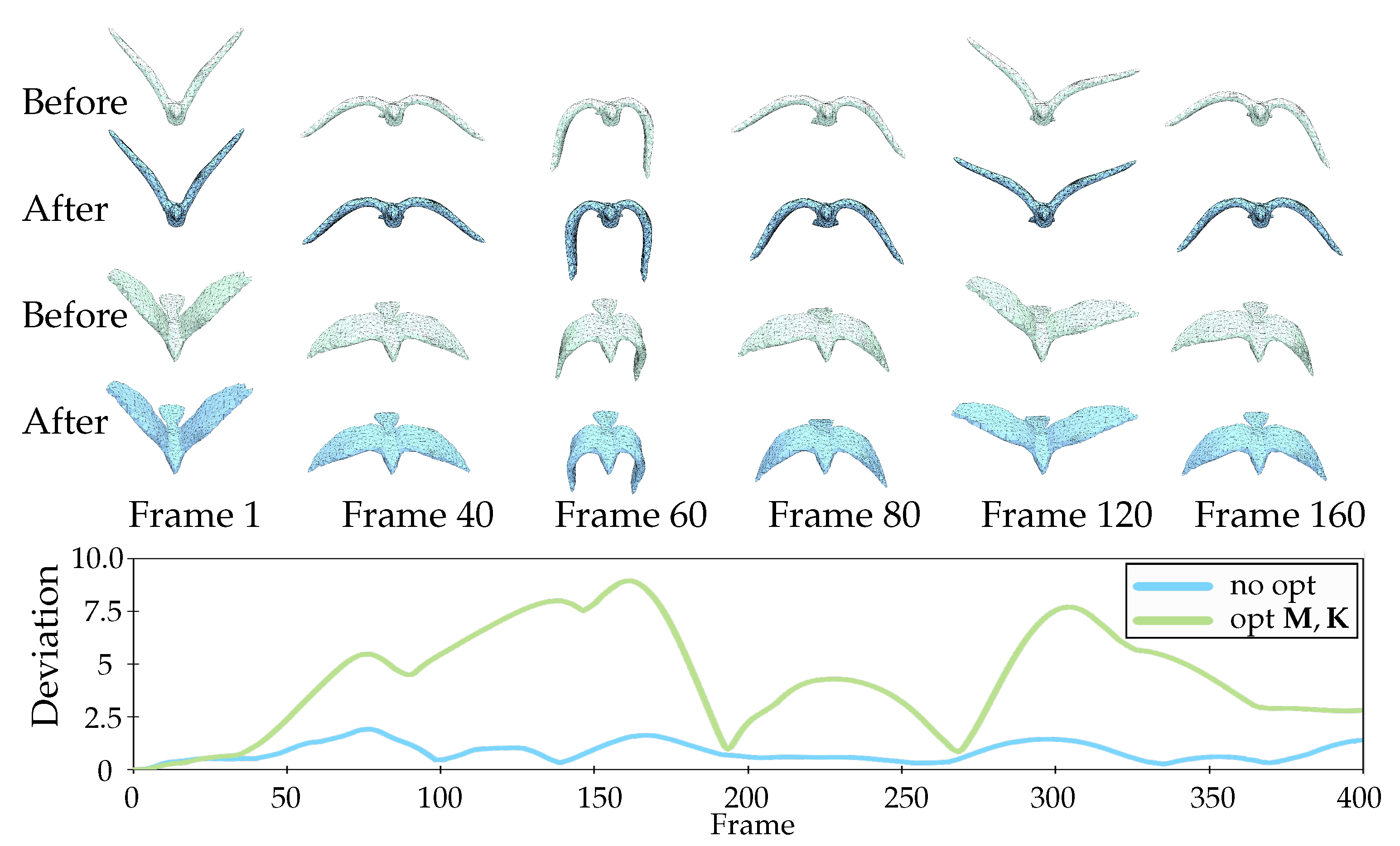
Firstly, we will show how such an additional mass rescaling helps to symmetrize the dynamic simulations in terms of shapes. Although the material optimization in our method is conducted based on the rest-state stiffness, we found that the material scalings are also applicable to co-rotational elasticity, which has the same underlying linear strain-stress relationship, but properly gets rid of rotations when computing the strain from displacements. In Figure 10, it is clear that directly simulating a bird flying with the original mesh causes obvious asymmetry along the dynamic sequence because of the asymmetry of the input mesh. Unlike static deformation, such discretization induced artifacts may become severe since they could be accumulated in the dynamic evolution. In contrast, our method managed to produce a far more symmetric co-rotational simulation in a completely automatic way.
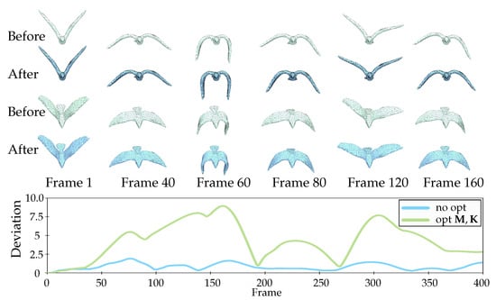
Figure 10.
We use a linear material with Poisson’s ratio and Young’s modulus . From two different camera views (top and bottom two rows, respectively), we can clearly see that the symmetry of the dynamics is preserved much better after optimizing both the elastic stiffness and mass scalings. Reflected in the numerical metrics, the symmetry error calculated by Equation (7) is reduced greatly along the entire simulation as depicted by the bottom chart, in which the blue curve is for the optimized result, while the green one is for the unoptimized result.
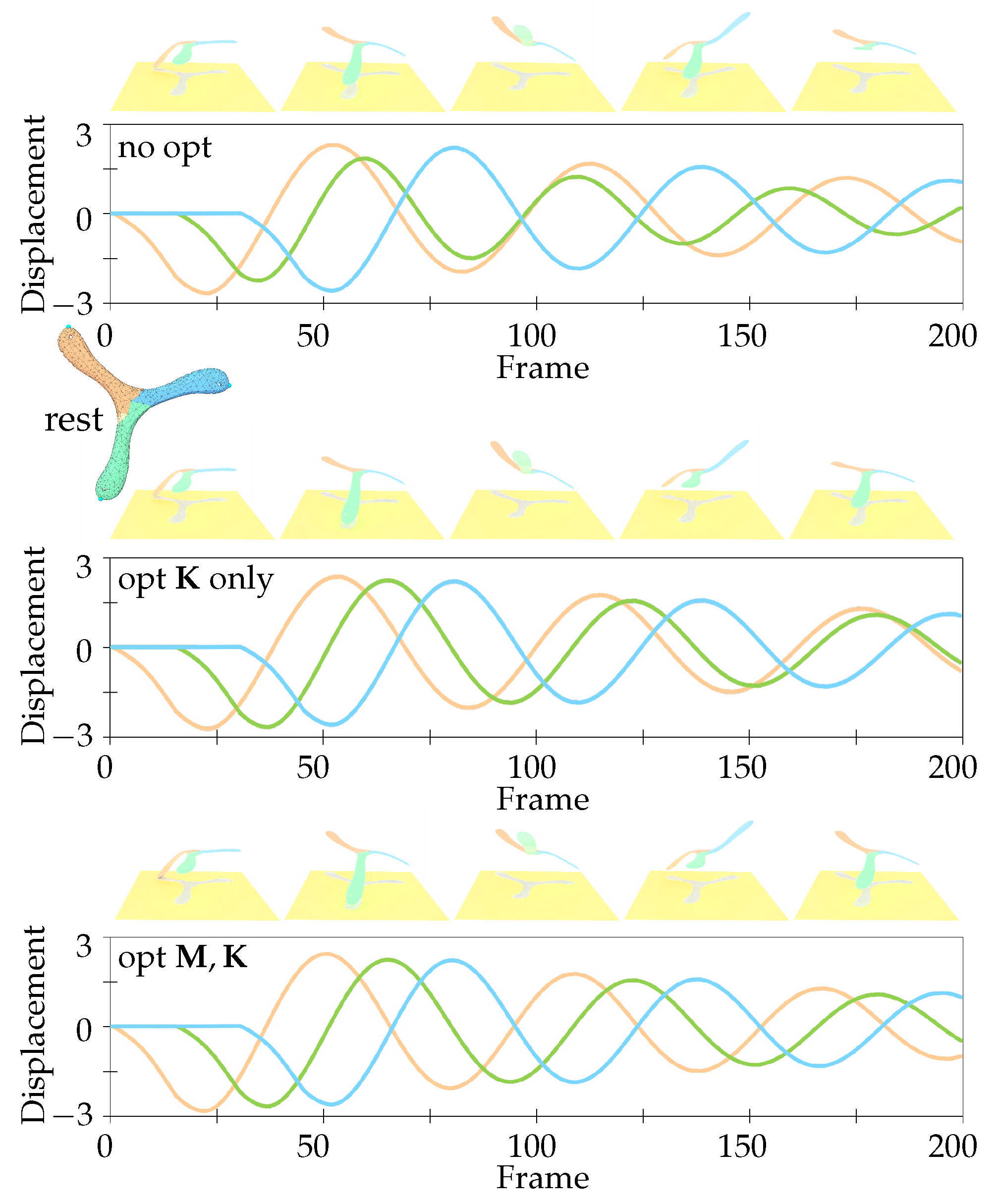
Figure 11 shows that our method can preserve the symmetry in the dynamic trajectory. We apply the same load on each wing of a fan model for an evenly spaced time duration as the initial condition. As illustrated in Figure 11, the dynamic trajectories show notable phase error without material optimization. The results are refined when the stiffness is optimized, and it keeps a significantly better symmetry in “phase” while both the mass and stiffness are optimized. Note that it is difficult or tedious for traditional methods to design special constraints or post-processing for this simulation.
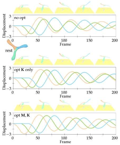
Figure 11.
After optimizing the stiffness and mass scaling sequentially (bottom row), the vibration amplitude and phase of each component are increasingly consistent compared to those without optimization (top row) and optimizing elastic stiffness only (middle row). The colored curves record the vertical displacements of three marker nodes (blue dots on the model) selected on each wing with the same color.
6. Conclusion and Future Work
In this paper, a material optimization method for symmetric models is proposed to rectify the unexpected asymmetry behavior caused by asymmetric meshes. Thanks to the method, the model discretized with the asymmetric mesh can be deformed into symmetric shapes under symmetric force fields in a static equilibrium state and exhibits symmetric kinematic behavior in the dynamic simulation. It saves the efforts of specially designing constraints and post-processing for kinematic symmetric behavior. Compared to those methods that simply increasing the density of the mesh or use higher order bases, our method brings a reduction of the computation time during the simulation.
Similar to most material optimization methods, the cost to adjust Young’s modulus and the mass is high, although it can be precomputed. The material is sensitive to the prescribed boundary conditions, and the simulation results may become asymmetric when applying different conditions. These two issues are indeed related. On the one hand, if material optimization is fast enough, one can integrate the costly pre-computation stage with the runtime simulation. To this end, ideas like reducing the material space [14,15] could be used. On the other hand, one can regress a function between the boundary conditions and the optimized materials and adapt the material according to the current boundary condition.
Author Contributions
Conceptualization, Z.S. and J.H.; formal analysis, Z.S. and J.C.; funding acquisition, Y.J.; software, J.L.; supervision, Y.J. and J.H.; writing—original draft, Z.S., J.L., and J.C.; writing—review and editing, Y.J. and J.H. All authors read and agree to the published version of the manuscript.
Funding
This work was supported in part by the National Natural Science Foundation of China (No. 61702458) and the 2011 Collaborative Innovation Center for Garment Personalized Customization of Zhejiang Province, China (No. 63, 2016).
Institutional Review Board Statement
Not applicable.
Informed Consent Statement
Not applicable.
Data Availability Statement
The data presented in this study are available on request from the corresponding author. The data are not publicly available due to usage restrictions.
Acknowledgments
We would like to thank the anonymous reviewers for their careful reading and valuable comments and suggestions.
Conflicts of Interest
The authors declare no conflict of interest.
Appendix A. Gradients
While calculating the derivatives of the regularization term is quite simple, it is more involved for the asymmetric energy term . Hence, we provide a detailed derivation here.
For clarity, let H denote the asymmetric energy term, and let , , so that . We number the elements in and let and denote the scaling coefficient and stiffness matrix for the i-th element, respectively. Together, we have:
Applying the chain rule, the gradient of H can be computed as:
Since , we have:
According to Equation (A1), we have:
Appendix B. Diagonal of the Approximate Hessian
To accelerate the convergence of the optimization by Equation (28), we use a simple preconditioner based on the diagonal entries of the Hessian matrix. Calculating the Hessian matrix of the regularization term is relatively easy, so we only provide the derivation for the asymmetric energy term. The same notations as in Appendix A are taken here. In the Hessian of H, each diagonal entry is written as . According to Equation (A2), we have:
By applying the chain rule and differentiating the matrix inverse, the above formula can be evaluated as:
So far, we have obtained the expression of each term in Equation (A6). The inverse diagonal of the approximate Hessian evaluated at is used for preconditioning all the L-BFGS iterations.
References
- Panozzo, D.; Lipman, Y.; Puppo, E.; Zorin, D. Fields on Symmetric Surfaces. ACM Trans. Graph. 2012, 31, 1–12. [Google Scholar] [CrossRef]
- Mitra, N.J.; Pauly, M.; Wand, M.; Ceylan, D. Symmetry in 3D Geometry: Extraction and Applications. Comput. Graph. Forum 2013, 32, 1–23. [Google Scholar] [CrossRef]
- Atallah, M.J. On Symmetry Detection. IEEE Trans. Comput. 1985, 34, 663–666. [Google Scholar] [CrossRef]
- Podolak, J.; Shilane, P.; Golovinskiy, A.; Rusinkiewicz, S.; Funkhouser, T. A Planar-Reflective Symmetry Transform for 3D Shapes. ACM Trans. Graph. 2006, 25, 549–559. [Google Scholar] [CrossRef]
- Mitra, N.J.; Guibas, L.J.; Pauly, M. Partial and Approximate Symmetry Detection for 3D Geometry. ACM Trans. Graph. 2006, 25, 560–568. [Google Scholar] [CrossRef]
- Shi, Z.; Alliez, P.; Desbrun, M.; Bao, H.; Huang, J. Symmetry and Orbit Detection via Lie-Algebra Voting; Eurographics Association: Goslar, Germany, 2016; pp. 217–227. [Google Scholar]
- Dessein, A.; Smith, W.A.P.; Wilson, R.C.; Hancock, E.R. Symmetry-Aware Mesh Segmentation into Uniform Overlapping Patches. Comput. Graph. Forum 2016, 36, 95–107. [Google Scholar] [CrossRef]
- Thrun, S.; Wegbreit, B. Shape from symmetry. In Proceedings of the Tenth IEEE International Conference on Computer Vision (ICCV’05), Beijing, China, 17–21 October 2005; Volume 2, pp. 1824–1831. [Google Scholar]
- Wang, Y.; Xu, K.; Li, J.; Zhang, H.; Shamir, A.; Liu, L.; Cheng, Z.Q.; Xiong, Y. Symmetry Hierarchy of Man-Made Objects. Comput. Graph. Forum 2011, 30, 287–296. [Google Scholar] [CrossRef]
- Chen, Y.; Song, Z.; Xu, W.; Martin, R.R.; Cheng, Z. Parametric 3D modeling of a symmetric human body. Comput. Graph. 2019, 81, 52–60. [Google Scholar] [CrossRef]
- Sifakis, E.; Barbič, J. Finite element method simulation of 3d deformable solids. Synth. Lect. Vis. Comput. Comput. Graph. Animat. Comput. Photogr. Imaging 2015, 1, 1–69. [Google Scholar] [CrossRef]
- Huang, J.; Chen, J.; Xu, W.; Bao, H. A survey on fast simulation of elastic objects. Front. Comput. Sci. 2019, 13, 443–459. [Google Scholar] [CrossRef]
- Bickel, B.; Bächer, M.; Otaduy, M.A.; Matusik, W.; Pfister, H.; Gross, M. Capture and Modeling of Non-Linear Heterogeneous Soft Tissue. ACM Trans. Graph. 2009, 28, 1–9. [Google Scholar] [CrossRef]
- Xu, H.; Li, Y.; Chen, Y.; Barbič, J. Interactive Material Design Using Model Reduction. ACM Trans. Graph. 2015, 34, 1–14. [Google Scholar] [CrossRef]
- Li, S.; Huang, J.; de Goes, F.; Jin, X.; Bao, H.; Desbrun, M. Space-Time Editing of Elastic Motion through Material Optimization and Reduction. ACM Trans. Graph. 2014, 33, 1–10. [Google Scholar] [CrossRef]
- Bickel, B.; Bächer, M.; Otaduy, M.A.; Lee, H.R.; Pfister, H.; Gross, M.; Matusik, W. Design and Fabrication of Materials with Desired Deformation Behavior. ACM Trans. Graph. 2010, 29, 1–10. [Google Scholar] [CrossRef]
- Cheng, L.; Zhang, P.; Biyikli, E.; Bai, J.; Robbins, J.; To, A. Efficient design optimization of variable-density cellular structures for additive manufacturing: Theory and experimental validation. Rapid Prototyp. J. 2017, 23, 660–677. [Google Scholar] [CrossRef]
- Wang, H.; O’Brien, J.F.; Ramamoorthi, R. Data-driven elastic models for cloth: Modeling and measurement. ACM Trans. Graph. (TOG) 2011, 30, 1–12. [Google Scholar]
- Lee, H.P.; Lin, M.C. Fast optimization-based elasticity parameter estimation using reduced models. Vis. Comput. 2012, 28, 553–562. [Google Scholar] [CrossRef]
- Weiss, S.; Maier, R.; Cremers, D.; Westermann, R.; Thuerey, N. Correspondence-Free Material Reconstruction using Sparse Surface Constraints. In Proceedings of the IEEE/CVF Conference on Computer Vision and Pattern Recognition, Seattle, WA, USA, 14–19 June 2020; pp. 4686–4695. [Google Scholar]
- Xu, H.; Sin, F.; Zhu, Y.; Barbič, J. Nonlinear material design using principal stretches. ACM Trans. Graph. (TOG) 2015, 34, 1–11. [Google Scholar] [CrossRef]
- Miguel, E.; Miraut, D.; Otaduy, M.A. Modeling and Estimation of Energy-Based Hyperelastic Objects. Comput. Graph. Forum 2016, 35, 385–396. [Google Scholar] [CrossRef]
- Akgün, M.A.; Garcelon, J.H.; Haftka, R.T. Fast exact linear and non-linear structural reanalysis and the Sherman–Morrison–Woodbury formulas. Int. J. Numer. Methods Eng. 2001, 50, 1587–1606. [Google Scholar] [CrossRef]
- Yan, G.; Li, W.; Yang, R.; Wang, H. Inexact descent methods for elastic parameter optimization. ACM Trans. Graph. (TOG) 2018, 37, 1–14. [Google Scholar] [CrossRef]
- Simari, P.; Kalogerakis, E.; Singh, K. Folding Meshes: Hierarchical Mesh Segmentation Based on Planar Symmetry. In Proceedings of the Fourth Eurographics Symposium on Geometry Processing; Eurographics Association: Goslar, Germany, 2006; pp. 11–119. [Google Scholar]
- Baraff, D.; Witkin, A. Large Steps in Cloth Simulation. In Proceedings of the 25th Annual Conference on Computer Graphics and Interactive Techniques; Association for Computing Machinery: New York, NY, USA, 1998; pp. 43–54. [Google Scholar]
- Bochkanov, S. ALGLIB. Version 3.16.0. 2019. Available online: www.alglib.net (accessed on 13 February 2021).
Publisher’s Note: MDPI stays neutral with regard to jurisdictional claims in published maps and institutional affiliations. |
© 2021 by the authors. Licensee MDPI, Basel, Switzerland. This article is an open access article distributed under the terms and conditions of the Creative Commons Attribution (CC BY) license (http://creativecommons.org/licenses/by/4.0/).

