Abstract
Heavy hadron spectroscopy was well understood within the naive quark model until the end of the past century. However, in 2003, the was discovered, with puzzling properties difficult to understand in the simple naive quark model picture. This state made clear that excited states of heavy mesons should be coupled to two-meson states in order to understand not only the masses but, in some cases, unexpected decay properties. In this work, we will give an overview of a way in which the naive quark model can be complemented with the coupling to two hadron thresholds. This program has been already applied to the heavy meson spectrum with the chiral quark model, and we show some examples where thresholds are of special relevance.
1. Introduction
Heavy hadron spectroscopy started in November 1974, when Brookhaven National Laboratory announced the discovery of a new particle called J [1] and, at the same time, the Stanford Linear Accelerator reported the existence of another new particle, called [2]. Very soon, both particles were seen as the same state, which we know now as the state of the charmonium spectrum. This state was understood as a bound state in the naive quark model, and its discovery was the confirmation of the existence of the charm quark that was predicted by the GIM mechanism [3] a few years before.
Afterwards, heavy meson spectroscopy developed very fast during the following years. The , the first state with bottom quarks discovered, was found at Fermilab [4] in 1977. Already in 1980, there were 11 new mesons included in the Particle Data Group (PDG) table [5] on these energy ranges, but that rate decreased to only 15 new states added during the period 1980 to 2003 [6]. However, during these last 17 years, 35 new states have been added [7], considering only unflavored mesons.
In the case of the baryon spectra, the first evidence of charmed baryons came six months after the discovery of the , in 1975 [8], but, in 1980, only the and baryons were included in the heavy baryon spectrum of the PDG [5]. In 2003, only 14 states were identified [6], while again, during the last 17 years, 33 new states have been included [7].
This impressive development of the heavy hadron spectrum has been possible thanks in part to the so called B-factories, like Belle and BaBar, which are electron–positron colliders tuned to the center of mass energy of the that decays into two B mesons. Other facilities like BESIII, with a lower energy electron–positron collider, have contributed. Many impressive results have also been obtained and are underway at LHC by the LHCb, CMS, and ATLAS Collaborations. The next generation SuperB-factory Belle II is running from 2018, and it is expected to make many important contributions to heavy hadron physics.
From a theoretical point of view, the description of the hadron spectroscopy has mostly relied on potential models since the discovery of the meson. Regarding heavy quarkonium spectroscopy, potential models have been very successful at describing the charmonium and bottomonium spectra (see, e.g., [9,10,11,12,13,14,15,16,17]). It is worth mentioning that new theoretical approaches directly derived from QCD, such as Effective Field Theories (EFTs) like non-relativistic QCD (NRQCD) [18,19,20] or lattice gauge theories [21,22,23] have been recently employed to study hadron spectroscopy. However, due to their complexity, many features of the hadron spectroscopy are more easily addressed with potential model approaches. Already in 1978, the Cornell model [24] was developed to understand heavy meson spectroscopy. This model is a non-relativistic approach for heavy quarks with interactions that are governed by color gauge symmetry, with the flavor only broken by the quark masses. The main pieces of the model are a Coulomb-like interaction, inspired by the one-gluon exchange, and a linear term, which describes the confining effect. It also took into account two important features that one expects from QCD, Heavy Flavor Symmetry (HFS) and Heavy Quark Spin Symmetry (HQSS), considering terms that are flavor and spin independent. The naive quark model from Cornell was fitted to the only 11 states that were known in 1978 and gave a quite good description of the charmonium and bottomonium spectrum at that time [25]. Not only that, the predictions were in quite good agreement with the experiments up to 2003, giving a prediction for 15 new states in the correct energy range. The Cornell potential has been related with the QCD static potential by Sumino [26] and more recently with NRQCD up to [27].
For the baryon spectra, also very soon, in 1979, quark models developed for the light sector were applied in the heavy quark sector [28]. In addition, Stanley and Robsen [29] extended the Cornell model to study heavy baryons. Many new states were predicted, but it took a long time to be seen on experiments.
Until 2003, the simple naive quark model picture was in quite good agreement with experiments. However, already in the original Cornell model [24], the coupling with two-meson thresholds was considered for excited states, although it was found to be of no relevance for the states considered at that time. The key event in 2003 for heavy hadron spectroscopy was the discovery of the by the Belle Collaboration [30]. It was very soon confirmed by the CDF [31], D0 [32], and BaBar [33] Collaborations. It has some intriguing properties that are difficult to understand in the naive quark model picture but easily explained when coupled channel effects are included.
Nevertheless, one of the clearest indications that coupled-channel effects have to be considered are the famous pentaquarks measured by LHCb [34,35]. These states are unflavored baryons in the region of GeV which rules out a three-light quark baryon interpretation. The only possible explanation is a pentaquark with three light quarks and a pair. Whether these states are compact pentaquarks or baryon-meson molecules is a matter of intense debate, although the closeness of these states to different meson–baryon thresholds is seen as a clear indication of the second possibility.
In this work, we will make a brief overview of coupled-channel effects in the framework of the quark model, in the same spirit as the original Cornell model. Thus, we will use naive quark-model states coupled to two-hadron channels, also built from naive quark-model states. The coupling between these two different sectors will be obtained using the microscopic creation model. The paper is organized as follows: In Section 2, we will give a brief introduction to the naive chiral quark model and how to calculate the spectrum in this picture. In Section 3, we will give the basis of the model and how to evaluate the transition amplitude. Section 4 will be devoted to present the formalism to couple one and two-hadron states. In Section 5, we will show a few examples in the meson spectrum where such effects are relevant and show some results in the quark model picture. We will end with some conclusions.
2. The Naive Chiral Quark Model
The quark model we use is a constituent quark model based on spontaneous chiral symmetry breaking [36]. It was first applied to the light-quark sector [37] and then extended to the heavy sector [38].
The main ingredients of the model are the following. The spontaneous chiral symmetry breaking generates two important effects in the light-quark sector. On one side, the light quarks acquire a dynamical mass that, at zero momentum, is of the order of 330 MeV for the u and d quarks, and 550 MeV for the s quark. This dynamical effect has been seen on the lattice [39], and it is the idea introduced phenomenologically in the constituent quark model. On the other side, it introduces the interaction of light quarks through the exchange of pseudo-Goldstone bosons. Another important non-perturbative effect is confinement, seen as the fact that hadrons are only seen in color singlets. We include it phenomenologically using a linear screened confinement interaction. This effect has also been observed in lattice QCD, where, in quenched QCD, a linear rising of the energy of two static sources with increasing distance is clearly seen [40] and, in unquenched QCD, this string is broken [41] when there is enough energy to produce a quark–antiquark pair. Finally, we introduce QCD perturbative effects through the one-gluon exchange interaction [42]. The model has been reviewed in many works, and all of the details can be found in Refs. [43,44].
Once the model interaction is settled, in order to obtain the hadron wave functions, one has to solve a non-relativistic bound equation for the two-body problem, in the case of mesons, as quark–antiquark pairs or the three body problem, for baryons, as three-quark states. There are many different approaches to solve these systems. The problem can be solved in coordinate space, in momentum space or using the Rayleigh–Ritz variational principle using a certain basis function. Sometimes, the potential involved poses special problems for some technique. For example, the use of a Coulomb-like potential makes the diagonal part of the potential in momentum space logarithmically divergent, which introduces a numerical problem. On the other hand, if we use a non-local interaction in coordinate space, the Schrödinger equation ends up being an integro-differential equation, which is also numerically more demanding. Another important fact is whether coupled channels are considered or not. Momentum space calculations or variational calculations are very easily extended to such a case, while coordinate space calculations are not straightforwardly extended.
Nonetheless, the method that can be usually used in any case is the variational method. This method is specially interesting for our purposes since we will be able to calculate transition amplitudes based on the model with matrix elements of the basis functions used.
The main problem of the method is to find the appropriate basis functions. There are many different options for many different systems. However, the Gaussian Expansion Method (GEM) has been shown to be a very good approach in almost any case. The method was firstly proposed by Kamimura [45] and has been applied to many few body problems [46,47].
In the case of the two-body problem, the employed basis functions are a set of Gaussians multiplied by a solid-spherical harmonic in the relative coordinate, to take into account the correct behavior of the wave function at the origin
The basis function is generated by taking several values for the Gaussian parameter . In the GEM, these parameters are taken in geometrical progression as
where and are the minimum and maximum radius and N the number of Gaussians. and should be chosen such that the range of the wave functions is well represented. For excited states, usually the range increases, so states with a higher range than will not be correctly represented. should be below the range of the potential. Numerically, it is important that the parameter a is not too close to 1 so that the problem does not become singular, so N can not be increased arbitrarily for fixed values of and . Then, one can use the expansion
and ends up with the generalized eigenvalue problem
with
In the case of the naive quark model, one has to include the spin–flavor–color degrees of freedom so the total wave function is
where is the spin wave function, is the flavor wave function, and is the color singlet quark–antiquark wave function and where the orbital angular momentum l is coupled with the spin S to total angular momentum J.
As a matter of fact, the GEM is more interesting when we have more than two interacting particles. Usually, one chooses a set of coordinates that includes the center of mass, so one solves for the relative motion of the interacting particles. Then, one builds the most general wave function with the desired total quantum numbers. This is usually done considering an expansion in angular momentum of the different coordinates and one assumes that, for short-range interactions, only the lowest partial waves will be needed. To have a feeling of what is needed, typical accurate three-body Fadeev calculations of Triton binding energy need up to 38 of such partial waves. The GEM approaches the problem in a different way; it also considers the lowest partial waves, although not only in one set of possible Jacobi coordinates, but in different sets. This has been shown to have a much faster convergence than the previous approach, which numerically is less demanding because radial wave functions in a lower number of partial waves are needed. The drawback is that now different partial waves are not orthogonal, so they cannot be considered separately.
In the case of the three-body problem, there are three different sets of Jacobi coordinates given by
where is the position vector of particle i, and is one of the three even permutations of . The orbital wave function is taken as
where gives the parity, and is the total orbital angular momentum. If there are identical particles, some relations between different modes i may be needed. These relations can be easily obtained from the action of the permutation operator
If we consider, for example, the Helium atom, with particle 1 being the nuclei and particles 2 and 3 the electrons, then we can consider two different wave functions with definite symmetry against the operator
where the symmetry to the exchange of the electrons is in the first case and for the second case. In principle, one could only work with one basis including all possible angular momentums but numerically is more efficient to use both with the lower angular momentum. Then, the spin wave functions of the electrons have to be considered to solve the wave functions for parahelium () and orthohelium (). In Table 1 and Table 2, we show the ground state and first excited states for parahelium and orthohelium, respectively, compared to experimental data from the NIST database. Here, we only include Coulomb interactions so we should expect deviations of the order of . As we can see, even with a long-range interaction such as the Coulomb one, the GEM works very well.

Table 1.
First levels of parahelium () with orbital angular momentum . The experimental data are taken from NIST, Ref. [48]—results with the GEM method from this work. All energies are in eV.
Table 2.
First levels of orthohelium () with orbital angular momentum . The experimental data are taken from NIST, Ref. [48]—results with the GEM method from this work. All energies are in eV.
If the three particles are identical, then the wave function to be used is
As explained above, we have to include the spin–flavor–color wave function for baryons in a quark model where, again, the spin is coupled with the total orbital angular momentum to give a total angular momentum J, and the color wave function corresponds to the color singlet.
The GEM is again very accurate and, in Table 3, we give the result of ground state heavy baryons in the Bhaduri [49] model, calculated with the GEM and compared with a Fadeev calculation by B. Silvestre-Brac [50]. The GEM calculation only includes wave functions with . In addition, the matter radius square and the charge radius square defined by
are given. From the results, one expects to have a good approximation to the solution of the three-body problem using the GEM.
Table 3.
Results for the Bhaduri potential obtained with a Fadeev calculation (FD) [50] and the GEM method (this work). Masses are given in MeV, while matter radius square and charge radius square are in fm.
However, not all the states are below the lowest open threshold. If we again consider the Helium atom, the first ionization occurs at an energy of eV [51], when the continuum of a ground state of a atom and a free electron starts. As the GEM takes boundary conditions for bound states, one can still find these bound states as shown in Table 4, although it is more difficult. These states can decay into a so they are resonances and can be seen on scattering processes. In the case of hadrons, there is a similar situation; however, quarks can not abandon a hadron, and a quark–antiquark pair is produced to generate two hadron states.
Table 4.
Levels of orthohelium () above the first open threshold. The experimental data are taken from NIST, Refs. [52,53]—results with the GEM method from this work. All energies are in eV.
3. The Model
The quark–pair creation model or model is a microscopic model that allows for coupling channels with different number of quarks (Figure 1). The name comes from the fact that a quark–antiquark pair is created with quantum numbers of the vacuum. It was first proposed by Micu [54] and, afterwards, Le Yaouanc et al. applied it to the strong decays of mesons [55] and baryons [56]. These authors also evaluated strong decay partial widths of the three charmonium states , , and within the same model [57,58].
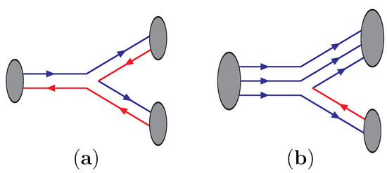
Figure 1.
Diagrams of the model that contributes to the decay of a meson into two mesons (a) and a baryon into a baryon and a meson (b).
The model is usually formulated in terms of the Hamiltonian operator
where the only parameter of the model is . The factor is usually not included, but, in our case, cancels the color factor in the meson sector, so has the usual definition.
It can be also formulated in terms of a transition operator given by
where are the spin, flavor, and color quantum numbers of the created quark (antiquark). The spin of the quark and antiquark is coupled to one. The is the solid harmonic defined as a function of the spherical harmonic.
It is common to give the transition operator in terms of the strength of the quark–antiquark pair creation from the vacuum as in Ref. [59]. The relation is given as
m being the mass of the pair created, which is usually a light pair.
We consider a process where an initial hadron A decays into two final hadrons B and C. When we work in the center of mass system of the initial hadron, we have , with the momentum of the initial hadron and the total momentum of the final hadrons. Then, the matrix element of the transition operator is written as
The matrix element is taken between hadron states written in terms of quark degrees of freedom in second quantization. Meson and baryon states are written as
where is a quark creation operator and an antiquark creation operator, is a factor in terms of the number of identical quarks in the baryon, and with the normalization convention for the wave functions,
where the sum is for discrete degrees of freedom. With these states, two hadron states with correct quantum numbers are constructed.
With the transition amplitude, the widths for strong decays can be evaluated
with the relative momentum of the two final hadrons.
The transition amplitude is basically given in terms of the wave function of the naive quark model considered. There are many factors that are given in terms of the quark model symmetries, but also an important form factor is given in terms of the overlap of the initial and final hadron wave functions with the transition operators. The orbital part of the matrix element can be difficult to compute, and this is the reason why the use of the GEM to solve the internal wave function of mesons and baryons is of special interest. The linearity of the operator allows that, using the expansion of the wave function in the GEM basis,
where , , and are the different GEM components for the hadrons and the c’s the coefficients for the solution of the GEM, one can evaluate the matrix element in terms of matrix elements in the GEM basis as
where the matrix elements in the GEM basis are evaluated analytically.
Once the naive quark model is fixed, the only unknown to determine the transition amplitude is the strength parameter . In the case of meson decays, a scale-dependent parameter was considered in Ref. [60] as
with and MeV. The scale is taken as the reduced mass of the quarks on the initial meson. The parameters were fixed to the strong width of a few open-charm, charmonium, and bottomonium states and, then, applied to many different states on these sectors. However, it is interesting to notice that this scale dependence was able to predict the strong decay widths of open-bottom mesons correctly without including this sector on the fit.
4. The Unquenched Quark Model
The unquenched quark model [61] or unitarized quark models [62] include the effects of two-hadron thresholds in one hadron state through hadron loops. They are usually implemented with approximate wave functions, and the interaction between the two-hadrons in the loops is not considered. Here, we present how these effects can be incorporated in an easy way.
In the previous section, we showed how one and two-hadron states are connected and give rise to the strong decay widths. However, the same transition amplitude has as a consequence: The one-hadron and two-hadron states connected gets mixed. As the origin is the strong force, this mixing can be sizable. For this reason, in some cases, it is important to consider the effect and, for this purpose, we consider the physical state as
where are naive quark model one-hadron states with quantum numbers and are two-hadron state with quantum numbers and relative momentum P. We define now the transition amplitude
If we impose the Schrödinger equation
and solve for the one-hadron amplitudes, we find
where is given by the equation in the two-hadron sector
Here, is the Hamiltonian generated by the kinetic energy of all the quarks and interaction between pairs of quarks that depend on the relative momentum of the hadrons, since the other degrees of freedom are fixed by the hadron states. There is also a part of the interaction which is generated by the coupling with one-hadron states and is given by
It is interesting to notice that this effective potential has special relevance at an energy close to the threshold of a two meson channel , , where one expects the molecules to appear. Furthermore, one should expect attraction for since and there is repulsion in the other case, it being more intense when the bare state is closer to the threshold . Thus, states above threshold will help to bind a molecule while states below threshold will help to unbind it. This analysis helps to know when a dynamically generated state can appear.
This formalism is suitable for bound states. However, in order to solve the scattering or consider resonances, it is convenient to work with the equivalent Lippmann–Schwinger equation written as
with
The solution to this equation is given in Ref. [63]
The first term on the right-hand side is the non-resonant contribution given by the solution of the equation
The resonant part include the dressed vertex functions
and the dressed two hadron propagator defined as the inverse of
The dressed propagator has singularities at the energies of the resonance states so, to find these energies, we solve the equation
Once the resonance energies are known, we find one-hadron amplitudes by solving
and the two-hadron wave function is given by
with . Notice that the normalization of the wave-function requires
The solution with naive quark model states is only exact if all the state are included. However, including only those states close to the energy range under consideration has been shown to be a good approximation. In Ref. [64], the unquenched quark model for charmonium mesons was considered but solving not only for the relative two-hadron wave function, but for the wave function of the meson as a meson, getting very similar results to the present approximation.
5. Coupled Channel Effects
As mentioned before, since 2003, it has been clear that the naive quark model is not enough to understand the heavy hadron spectra. In some cases, such as the pentaquarks, the energy scale of its mass makes it unavoidable to include higher Fock components. However, as we will see, in other cases, threshold effects can easily explain properties that are very difficult to understand in the naive quark model. In this section, we give a few examples of such cases and we will summarize results obtained using the model previously introduced.
5.1. Isospin Breaking Effects
The was discovered in the invariant mass distribution of the decay. The two-pions in this decay came from a meson [65], which is an isospin 1 final state. The ratio of the decay into three pions was also measured, and the three-pions came from the decay of an meson [66], which is an isospin 0 channel. The ratio between these two decay modes was found to be
Thus, this state can decay into final states with two different values of isospin, which implies that either isospin is violated in the decay process or the isospin of the is not well defined.
The is now included in the PDG as the . Quark models usually predict this state at higher energies, although the deviation can be explained if one considers that this theoretical state is close and above the threshold. One important question is whether the is the state expected in this energy region by quark models, or if it is an additional state dynamically generated in the channel. In any case, the crucial property of this state is that its mass is very close to the with a binding energy given by
where the first number is from Ref. [67], the second from Ref. [68], and the third is from Ref. [69].
Since the mass is so close to the threshold, one would expect a molecule or a mixing with some charmonium state. Considering the large isospin breaking, the most promising source is the mass splitting between charge and neutral states of D and mesons, finding
to be a larger scale than the binding energy, which suggests a big effect. Notice that the masses by themselves do not suggest it, since the breaking is only of and for the D and mesons, respectively. This effect was introduced by Swanson [70] in a coupled channel calculation in which an isospin 1 channel was introduced. The important point to notice is that the binding energy for the charged channel is around 8 MeV, so the size of this component is around fm, while, for the neutral, the small binding energy B makes the size of the order of 4 fm or bigger. This effect generates a big isospin breaking on the wave function out of the interaction region. This assertion generated some confusion since the isospin breaking effect is small in the interaction region. The isospin breaking was further analyzed in Ref. [71] in the framework of an Effective Field Theory, where the coupling of the states to the different final channels could be evaluated. The couplings obtained for states were MeV and MeV for charged and neutral channels, respectively, showing an isospin breaking of less than . In fact, although the ratio given in Equation (56) suggests a big isospin breaking, this is only due to the big phase space effects that enhances the isospin 1 channel against the isospin 0 [71]. Excluding phase space effects, the decay in the channel is only around of the channel decay. This was clarified in Ref. [72] relating the couplings with the probability of the wave function in the interacting region.
The microscopic calculation at the quark level was performed in Ref. [73] in the framework of the chiral quark model previously described. Within the model, the naive quark model state has a mass of 3947 MeV, which is far above the . Coupling with states makes the naive quark model masses change slightly. However, the important effect is that a new state appears in the threshold with properties in overall good agreement with those of the . This is in contrast to other unquenched quark models [74] where the is not an additional state but just a corrected naive quark model state by two meson loops.
The ratio of Equation (56) was analyzed in Ref. [75], finding a value close to the experimental result. The big isospin breaking on the wave function is represented in Figure 2. For exact isospin symmetry, the charged and neutral components should have the same probabilities, while we see that, close to the neutral threshold, this component dominates.
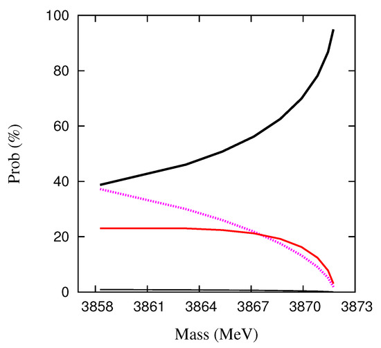
Figure 2.
Probabilities of different components in the physical state obtained in the unquenched chiral quark model as a function of the mass. The mass is varied using the strength parameter. Lines are , charged neutral in black and charged channel in red, in dashed magenta and in thin black.
This effect, seen on the state, may appear in any hadron–hadron molecule close to the threshold. Of particular interest are the famous pentaquark states [34,35], which are close to the , , and thresholds. This is the reason why it is widely accepted that the nature of these states is more likely to be a hadron–hadron molecule than a compact pentaquark state. Being close to the threshold, isospin breaking effects were studied [76], and these effects could be magnified in the [77]. For this state, the binding energy is MeV for the charged channel with lower threshold and MeV for the higher threshold. Analogously to the decays into and , the pentaquark could decay into an isospin channel or an isospin channel . Within an EFT framework, the ratio
was evaluated and showed to be up to . The measurement of this isospin violating decay of the pentaquark could be the best indication of its molecular nature.
5.2. HQSS and HFS Breaking
Heavy Quark Spin Symmetry (HQSS) and Heavy Flavor Symmetry (HFS) are good approximate symmetries of QCD, so one would expect them to be realized in the heavy hadron spectrum.
If we look into the heavy-light sector, under exact HQSS, the D and mesons should have the same mass. Despite it not exactly being realized, the ratio shows that the breaking is, indeed, small. In the hidden charm sector, we have and , so even smaller breaking. HFS implies that interactions do not depend on the heavy quark mass, so, when we find a state in the charm sector, there must exist an analog in the bottom sector.
If we consider the to be a molecule, HQSS [78,79,80] leads to unavoidable predictions. The interaction between and channels is the same, so, if the is a molecule, it implies that there should be a bound state with very similar binding energy in the , which was dubbed . In addition, HFS requires the interaction between charmed mesons to be the same as for bottom mesons [81], so the same molecules observed in the hidden-charm sector should appear in the hidden-bottom sector.
HQSS is usually fulfilled by heavy quark models, since the heavy quark mass only appears in fine structure terms that are suppressed as corrections. Within HQSS, one finds for S partial-waves [82]
where H represents the interacting Hamiltonian. In the chiral quark model of previous sections, the results for diagonal matrix elements are shown in Figure 3 and Figure 4, showing that HQSS is approximately fulfilled. Additionally, comparing the matrix elements of the interactions in the charmed and bottom sectors, we can see that HFS is also fulfilled.
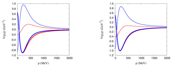
Figure 3.
Diagonal matrix elements of the two meson interaction in momentum space for the sector (left panel) and sector (right panel). For the left panel, the dashed blue line gives the matrix element, the dashed red line the , the solid blue line the right-hand side of Equation (61), and the solid red line left-hand side of the same equation. For the right panel, it is the same but for channels.
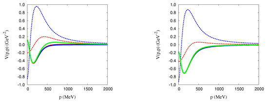
Figure 4.
Diagonal matrix elements of the two meson interaction in momentum space for the sector (left panel) and sector (right panel). For the left panel, the dashed blue line gives the matrix element, the dashed red line the , the solid blue line the right-hand side of Equation (62), the solid red line the left-hand side of the same equation, and the solid green line the right-hand side of Equation (63). At exact HQSS, the three solid lines should be equal. For the right panel, it is the same but for channels.
Nevertheless, open thresholds appear in energy regions where we can also find naive quark model states, so one-hadron and two-hadron states can be mixed as shown in the previous sections. This effect can have important consequences for states that are mainly dynamically generated molecules. Let’s see an example and consider the P-wave charmonium states. Considering the allowed spins, using the spectroscopic notation , we may have the states (), (), () and () coupled to . Under HQSS, all these states are degenerated (within a small deviation due to the breaking). The largest mass splitting is given by the difference of the ground states MeV, the splitting for excited states being smaller in the naive quark model picture. The and states are in the region of the thresholds; however, the threshold difference MeV is larger. Taking only S-wave two-meson states, only and can have quantum numbers, while only can have and can have . This means that the relevant threshold in each channel will have a different relative position with respect to naive quark model states. This is shown in Figure 5, where we can see that, for the channel, the naive quark model state is above the threshold, giving additional attraction, while, in the channel, the P-wave state is below the threshold, giving repulsion (The state above threshold is an F state.). This explains why the channel has an additional state, while the does not, which is against HQSS expectations. A systematic study of this effect was performed at the hadron level in Ref. [83], and a more elaborate study at the quark level was performed in Ref. [84].
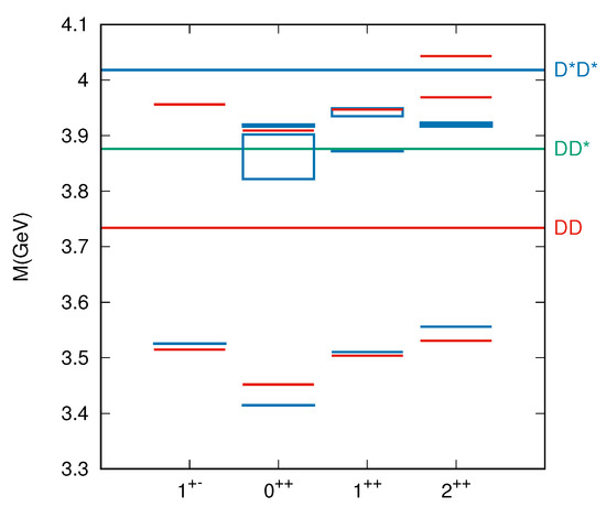
Figure 5.
Charmonium spectrum in the energy region of and states. Blue boxes show the states in the Particle Data Group [7]. The has been included in the and in the channels since the J quantum number is not known. The quantum numbers of the are also not known, but it has been included in the channel since it has been seen in but not in . The states in red are naive states predicted by the model.
In bottomonium, we have a different situation. In the channel, the naive quark model state generates repulsion and no additional state appears, while, in the channel, there is attraction from the state above threshold and repulsion from the state below, and the final result is that an additional state appears. This result is, again, against HFS expectations [82]. A more elaborate calculation including more thresholds is underway (Figure 6).
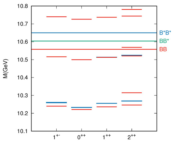
Figure 6.
Bottomonium spectrum in the energy region of and states. Blue boxes show the states in the Particle Data Group [7]. The states in red are the pure states predicted by the model.
5.3. Threshold Cusps
These are enhancements of the cross sections near the opening of a threshold. One famous example is the measurement of the scattering lengths difference in scattering using a cusp-like enhancement in the invariant mass distribution in the decay [85]. It was first noticed in Ref. [86] and then proposed to be measured by Cabibbo [87]. Due to the very precise experimental data available, a very precise determination of this combination was performed [88] that was in very good agreement with PT predictions.
This effect has been also used to explain strong energy dependencies near the threshold of invariant mass distributions, as in the case of and states [89,90]. The effect should be present when the interaction is attractive [91]; however, it has been argued [92] that such big effects may not appear without the existence of a nearby pole (bound, virtual, or resonance state).
One example of a threshold cusp effect in the hidden-charm sector is the resonance, a structure observed in the invariant mass spectrum by many collaborations, such as CDF [93], D0 [94], CMS [95], Belle [96], BaBar [97], and LHCb [98]. Within the chiral quark model described above, a coupled calculation of the main open-charm channels [99] showed that the structure just above the threshold is not caused by the effect of a nearby pole, but it is associated with the presence of the channel. The residual interaction is strong enough to show a rapid increase of the experimental counts, but too weak to develop a bound or virtual state.
Even more interesting is the case of and states. For the Zc(3900), there exist analyses of the BESIII data considering two-body coupled channels and triangle singularities [100,101,102]. In the chiral quark model, the states have been studied in Ref. [103]. The and are meson states in the charmonium energy range. The fact that they are charged rules out the possibility of being states, and, at least, four quarks are needed. The nature of these charged states is still an open question.
The was discovered by the BESIII [104] and Belle [105] Collaborations in the invariant mass distribution of the reaction . It was then seen by the BESIII Collaboration [106] in the invariant mass distribution of the reaction with a lower mass and was referred to as the , although now it is seen as the same state. Soon after this discovery, the BESIII Collaboration reported the discovery of another charged state, the , in the reaction [107]. Later on, BESIII also reported about the neutral partner [108], completing the isospin triplet.
In Ref. [103], was analyzed in the sector , within the formalism previously mentioned. Although here there is no state coupled to two-meson components, this system is interesting for another reason. There are two close-by channels that one would not expect to have an important effect, the and , since the interactions between these mesons are expected to be small. However, the non-diagonal interaction and are dominant, and they do not generate bound states but virtual states.
In Table 5, we give the pole position for the states corresponding to the and . The poles are below the and thresholds, respectively, and in the second Riemann sheet corresponding to virtual states. Despite these poles already emerging when the main open-charm channels are included, other channels are important in order to describe the experimental lineshapes. Lineshapes for different reactions are shown in Figure 7 and Figure 8. Although we find poles on the S-matrix that produce structures in the lineshapes, in some cases, they don’t seem enough, which supports the idea that a threshold cusp effect might not be sufficient to describe the experimental data without the existence of some associated pole.
Table 5.
The S-matrix pole positions, in , for different coupled-channels calculations [103]. The included channels for each case are shown in the first column. Poles are given in the second and fourth columns by the value of the complex energy in a specific Riemann sheet (RS). The RS columns indicate whether the pole has been found in the first (F) or second (S) Riemann sheet of a given channel. Each channel in the coupled-channels calculation is represented as an array’s element, ordered with increasing energy.
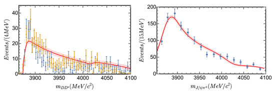
Figure 7.
Line shapes for (left panel) and (right panel) at GeV [103]. Experimental data are from Refs. [109,110], respectively. The theoretical line shapes have been convoluted with the experimental resolution. The line-shape’s uncertainty is shown as a shadowed area.
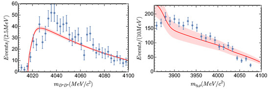
Figure 8.
Line shapes for (left panel) and (right panel) at GeV [103]. Experimental data for are from Ref. [111]. The theoretical line shapes have been convoluted with the experimental resolution. The line-shape’s -uncertainty is shown as a shadowed area.
6. Conclusions
The naive quark model has been very successful in describing heavy hadron phenomenology for a very long time. However, since 2003, it seems clear that the coupling with two hadron states are of relevance to describe the phenomenology of new discovered states.
In this work, we have described how a microscopic quark model can be used, and, in particular, the chiral quark model, to describe systems in which conventional quark model states can couple to two-hadron states in a consistent framework. Although these effects are of no relevance in many low-lying states, keeping the validity of the naive quark model, in some cases, the effects can be very important.
This framework has been used during the last few years to study the meson spectrum, and we have shown a few examples where deviations from naive quark model expectations are of special relevance. In fact, threshold effects can generate deviations from expected results predicted by well-known symmetries such as HFS or HQQS, highlighting the importance of analyzing such effects especially in the heavy meson and baryon sectors.
Author Contributions
Conceptualization and methodology, P.G.O. and D.R.E.; Software, P.G.O. and D.R.E.; Validation, P.G.O. and D.R.E.; Writing—original draft preparation, P.G.O. and D.R.E.; Writing—re-view and editing, P.G.O. and D.R.E.; Funding acquisition, P.G.O. and D.R.E.; All authors have read and agreed to the published version of the manuscript.
Funding
This work has been funded by the Ministerio de Economía, Industria y Competitividad under Contract No. FPA2016-77177-C2-2-P and Ministerio de Ciencia, Innovación y Universidades under Contract No. PID2019-105439GB-C22, and by the EU Horizon 2020 research and innovation program, STRONG-2020 project, under Grant No. 824093.
Institutional Review Board Statement
Not applicable.
Informed Consent Statement
Not applicable.
Data Availability Statement
Not applicable.
Conflicts of Interest
The authors declare no conflict of interest. The funders had no role in the design of the study; in the collection, analyses, or interpretation of data; in the writing of the manuscript, or in the decision to publish the results.
Abbreviations
The following abbreviations are used in this manuscript:
| HQQS | Heavy Quark Spin Symmetry |
| HFS | Heavy Flavor Symmetry |
| PT | Chiral Perturbation Theory |
| QCD | Quantum Chromodynamics |
References
- Aubert, J.J.; Becker, U.; Biggs, P.J.; Burger, J.; Chen, M.; Everhart, G.; Goldhagen, P.; Leong, J.; McCorriston, T.; Rhoades, T.G.; et al. Experimental Observation of a Heavy Particle J. Phys. Rev. Lett. 1974, 33, 1404–1406. [Google Scholar] [CrossRef]
- Augustin, J.E.; Boyarski, A.M.; Breidenbach, M.; Bulos, F.; Dakin, J.T.; Feldman, G.J.; Fischer, G.E.; Fryberger, D.; Hanson, G.; Jean-Marie, B.; et al. Discovery of a Narrow Resonance in e+e− Annihilation. Phys. Rev. Lett. 1974, 33, 1406–1408. [Google Scholar] [CrossRef]
- Glashow, S.L.; Iliopoulos, J.; Maiani, L. Weak Interactions with Lepton-Hadron Symmetry. Phys. Rev. D 1970, 2, 1285–1292. [Google Scholar] [CrossRef]
- Herb, S.W.; Hom, D.C.; Lederman, L.M.; Sens, J.C.; Snyder, H.D.; Yoh, J.K.; Appel, J.A.; Brown, B.C.; Brown, C.N.; Innes, W.R.; et al. Observation of a Dimuon Resonance at 9.5 GeV in 400-GeV Proton-Nucleus Collisions. Phys. Rev. Lett. 1977, 39, 252–255. [Google Scholar] [CrossRef]
- Kelly, R.L.; Horne, C.P.; Losty, M.J.; Rittenberg, A.; Shimada, T.; Trippe, T.G.; Wohl, C.G.; Yost, G.P.; Barash-Schmidt, N.; Bricman, C.; et al. Review of particle properties. Rev. Mod. Phys. 1980, 52, S1–S286. [Google Scholar] [CrossRef]
- Hagiwara, K.; Montanet, L.; Barnett, R.M.; Groom, D.E.; Trippe, T.G.; Wohl, C.G.; Armstrong, B.; Wagman, G.S.; Murayama, H.; Stone, J.; et al. Review of Particle Properties. Phys. Rev. D 2002, 66, 010001. [Google Scholar] [CrossRef]
- Particle Data Group; Zyla, P.A.; Barnett, R.M.; Beringer, J.; Dahl, O.; Dwyer, D.A.; Groom, D.E.; Lin, C.J.; Lugovsky, K.S.; Pianori, E.; et al. Review of Particle Physics. Prog. Theor. Exp. Phys. 2020, 2020, 083C01. [Google Scholar] [CrossRef]
- Cazzoli, E.G.; Cnops, A.M.; Connolly, P.L.; Louttit, R.I.; Murtagh, M.J.; Palmer, R.B.; Samios, N.P.; Tso, T.T.; Williams, H.H. Evidence for ΔS=−ΔQ Currents or Charmed-Baryon Production by Neutrinos. Phys. Rev. Lett. 1975, 34, 1125–1128. [Google Scholar] [CrossRef]
- Eichten, E.; Gottfried, K.; Kinoshita, T.; Lane, K.D.; Yan, T.M. Charmonium: The Model. Phys. Rev. D 1978, 17, 3090–3117, Erratum in 1980, 21, 313. [Google Scholar] [CrossRef]
- Eichten, E.; Gottfried, K.; Kinoshita, T.; Lane, K.D.; Yan, T.M. Charmonium: Comparison with Experiment. Phys. Rev. D 1980, 21, 203–233. [Google Scholar] [CrossRef]
- Gupta, S.N.; Radford, S.F.; Repko, W.W. Semirelativistic Potential Model for Charmonium. Phys. Rev. D 1985, 31, 160. [Google Scholar] [CrossRef] [PubMed]
- Barnes, T.; Close, F.E.; Page, P.R.; Swanson, E.S. Higher quarkonia. Phys. Rev. D 1997, 55, 4157–4188. [Google Scholar] [CrossRef]
- Ebert, D.; Faustov, R.N.; Galkin, V.O. Properties of heavy quarkonia and Bc mesons in the relativistic quark model. Phys. Rev. D 2003, 67, 014027. [Google Scholar] [CrossRef]
- Eichten, E.; Godfrey, S.; Mahlke, H.; Rosner, J.L. Quarkonia and their transitions. Rev. Mod. Phys. 2008, 80, 1161–1193. [Google Scholar] [CrossRef]
- Danilkin, I.V.; Simonov, Y.A. Channel coupling in heavy quarkonia: Energy levels, mixing, widths and new states. Phys. Rev. D 2010, 81, 074027. [Google Scholar] [CrossRef]
- Ferretti, J.; Santopinto, E. Higher mass bottomonia. Phys. Rev. D 2014, 90, 094022. [Google Scholar] [CrossRef]
- Godfrey, S.; Moats, K. Bottomonium Mesons and Strategies for their Observation. Phys. Rev. D 2015, 92, 054034. [Google Scholar] [CrossRef]
- Caswell, W.E.; Lepage, G.P. Effective Lagrangians for Bound State Problems in QED, QCD, and Other Field Theories. Phys. Lett. B 1986, 167, 437–442. [Google Scholar] [CrossRef]
- Pineda, A.; Soto, J. Effective field theory for ultrasoft momenta in NRQCD and NRQED. Nucl. Phys. B Proc. Suppl. 1998, 64, 428–432. [Google Scholar] [CrossRef]
- Brambilla, N.; Pineda, A.; Soto, J.; Vairo, A. Effective Field Theories for Heavy Quarkonium. Rev. Mod. Phys. 2005, 77, 1423. [Google Scholar] [CrossRef]
- Dudek, J.J.; Edwards, R.G.; Mathur, N.; Richards, D.G. Charmonium excited state spectrum in lattice QCD. Phys. Rev. D 2008, 77, 034501. [Google Scholar] [CrossRef]
- Gray, A.; Allison, I.; Davies, C.T.H.; Dalgic, E.; Lepage, G.P.; Shigemitsu, J.; Wingate, M. The Upsilon spectrum and m(b) from full lattice QCD. Phys. Rev. D 2005, 72, 094507. [Google Scholar] [CrossRef]
- Meinel, S. The Bottomonium spectrum from lattice QCD with 2+1 flavors of domain wall fermions. Phys. Rev. D 2009, 79, 094501. [Google Scholar] [CrossRef]
- Gottfried, K. The spectroscopy of massive quark-antiquark systems, Progress in Particle and Nuclear Physics. Prog. Part. Nucl. Phys. 1982, 8, 49–71. [Google Scholar] [CrossRef]
- Gostev, V.B.; Mineev, V.S.; Frenkin, A.R. The inverse problem of quantum mechanics for a linear potentia. Theor. Math. Phys. 1983, 56, 682–686. [Google Scholar] [CrossRef]
- Sumino, Y. QCD potential as a “Coulomb-plus-linear” potential. Phys. Lett. B 2003, 571, 173–183. [Google Scholar] [CrossRef]
- Mateu, V.; Ortega, P.G.; Entem, D.R.; Fernández, F. Calibrating the Naïve Cornell Model with NRQCD. Eur. Phys. J. C 2019, 79, 323. [Google Scholar] [CrossRef]
- Copley, L.A.; Isgur, N.; Karl, G. Charmed baryons in a quark model with hyperfine interactions. Phys. Rev. D 1979, 20, 768–775. [Google Scholar] [CrossRef]
- Stanley, D.P.; Robsen, D. Do Quarks Interact Pairwise and Satisfy the Color Hypothesis? Phys. Rev. Lett. 1980, 45, 235–238. [Google Scholar] [CrossRef]
- Choi, S.K.; Olsen, S.L.; Abe, K.; Abe, T.; Adachi, I.; Ahn, B.S.; Aihara, H.; Akai, K.; Akatsu, M.; Akemoto, M.; et al. Observation of a Narrow Charmoniumlike State in Exclusive B±→K±π+π−J/ψ Decays. Phys. Rev. Lett. 2003, 91, 262001. [Google Scholar] [CrossRef] [PubMed]
- Acosta, D.; Affolder, T.; Ahn, M.H.; Akimoto, T.; Albrow, M.G.; Ambrose, D.; Amerio, S.; Amidei, D.; Anastassov, A.; Anikeev, K.; et al. Observation of the Narrow State X(3872)→J/ψπ+π− in Collisions at = 1.96 TeV. Phys. Rev. Lett. 2004, 93, 072001. [Google Scholar] [CrossRef]
- Abazov, V.M.; Abbott, B.; Abolins, M.; Acharya, B.S.; Adams, D.L.; Adams, M.; Adams, T.; Agelou, M.; Agram, J.L.; Ahmed, S.N.; et al. Observation and Properties of the X(3872) Decaying to J/ψπ+π− in Collisions at = 1.96 TeV. Phys. Rev. Lett. 2004, 93, 162002. [Google Scholar] [CrossRef]
- Aubert, B.; Barate, R.; Boutigny, D.; Couderc, F.; Gaillard, J.M.; Hicheur, A.; Karyotakis, Y.; Lees, J.P.; Tisserand, V.; Zghiche, A.; et al. Study of the B−→J/ψK−π+π− decay and measurement of the B−→X(3872)K− branching fraction. Phys. Rev. D 2005, 71, 071103. [Google Scholar] [CrossRef]
- Aaij, R.; Adeva, B.; Adinolfi, M.; Affolder, A.; Ajaltouni, Z.; Akar, S.; Albrecht, J.; Alessio, F.; Alexander, M.; Ali, S.; et al. Observation of J/ψp Resonances Consistent with Pentaquark States in →J/ψK−p Decays. Phys. Rev. Lett. 2015, 115, 072001. [Google Scholar] [CrossRef]
- Aaij, R.; Beteta, C.A.; Adeva, B.; Adinolfi, M.; Aidala, C.A.; Ajaltouni, Z.; Akar, S.; Albicocco, P.; Albrecht, J.; Alessio, F.; et al. Observation of a Narrow Pentaquark State, Pc(4312)+, and of the Two-Peak Structure of the Pc(4450)+. Phys. Rev. Lett. 2019, 122, 222001. [Google Scholar] [CrossRef] [PubMed]
- Manohar, A.; Georgi, H. Chiral quarks and the non-relativistic quark model. Nucl. Phys. B 1984, 234, 189–212. [Google Scholar] [CrossRef]
- Fernandez, F.; Valcarce, A.; Straub, U.; Faessler, A. The nucleon-nucleon interaction in terms of quark degrees of freedom. J. Phys. G Nucl. Part. Phys. 1993, 19, 2013–2026. [Google Scholar] [CrossRef]
- Vijande, J.; Fernández, F.; Valcarce, A. Constituent quark model study of the meson spectra. J. Phys. G Nucl. Part. Phys. 2005, 31, 481–506. [Google Scholar] [CrossRef]
- Burgio, G.; Schröck, M.; Reinhardt, H.; Quandt, M. Running mass, effective energy, and confinement: The lattice quark propagator in Coulomb gauge. Phys. Rev. D 2012, 86, 014506. [Google Scholar] [CrossRef]
- Bali, G.S. QCD forces and heavy quark bound states. Phys. Rep. 2001, 343, 1–136. [Google Scholar] [CrossRef]
- Bali, G.S.; Neff, H.; Düssel, T.; Lippert, T.; Schilling, K. Observation of string breaking in QCD. Phys. Rev. D 2005, 71, 114513. [Google Scholar] [CrossRef]
- De Rújula, A.; Georgi, H.; Glashow, S.L. Hadron masses in a gauge theory. Phys. Rev. D 1975, 12, 147–162. [Google Scholar] [CrossRef]
- Segovia, J.; Yasser, A.M.; Entem, D.R.; Fernández, F. JPC=1−− hidden charm resonances. Phys. Rev. D 2008, 78, 114033. [Google Scholar] [CrossRef]
- Segovia, J.; Entem, D.R.; Fernandez, F.; Hernandez, E. Constituent quark model description of charmonium phenomenology. Int. J. Mod. Phys. E 2013, 22, 1330026. [Google Scholar] [CrossRef]
- Kamimura, M. Nonadiabatic coupled-rearrangement-channel approach to muonic molecules. Phys. Rev. A 1988, 38, 621–624. [Google Scholar] [CrossRef] [PubMed]
- Hiyama, E.; Kino, Y.; Kamimura, M. Gaussian expansion method for few-body systems. Prog. Part. Nucl. Phys. 2003, 51, 223–307. [Google Scholar] [CrossRef]
- Hiyama, E. Gaussian expansion method for few-body systems and its applications to atomic and nuclear physics. Prog. Theor. Exp. Phys. 2012, 2012, 01A204. [Google Scholar] [CrossRef]
- Morton, D.; Wu, Q.; Drake, G.W. Energy Levels for the Stable Isotopes of Atomic Helium (4He I and 3He I). Can. J. Phys. 2006, 84, 83–105. [Google Scholar] [CrossRef]
- Bhaduri, R.K.; Cohler, L.E.; Nogami, Y. A unified potential for mesons and baryons. Il Nuovo Cimento A 1981, 65. [Google Scholar] [CrossRef]
- Silvestre-Brac, B. Spectrum and Static Properties of Heavy Baryons. Few-Body Syst. 1996, 20. [Google Scholar] [CrossRef]
- Kandula, D.Z.; Gohle, C.; Pinkert, T.J.; Ubachs, W.; Eikema, K.S.E. Extreme Ultraviolet Frequency Comb Metrology. Phys. Rev. Lett. 2010, 105, 063001. [Google Scholar] [CrossRef] [PubMed]
- Martin, W.C. Energy Levels of Neutral Helium (4He I). J. Phys. Chem. Ref. Data 1973, 2, 257–266. [Google Scholar] [CrossRef]
- Tech, J.L.; Ward, J.F. Accurate Wavelength Measurement of the 1s2p3P0 − 2p23P Transition in 4He I. Phys. Rev. Lett. 1971, 27, 367–370. [Google Scholar] [CrossRef]
- Micu, L. Decay rates of meson resonances in a quark model. Nucl. Phys. 1969, B10, 521–526. [Google Scholar] [CrossRef]
- Le Yaouanc, A.; Oliver, L.; Pène, O.; Raynal, J.C. “Naive” Quark-Pair-Creation Model of Strong-Interaction Vertices. Phys. Rev. D 1973, 8, 2223–2234. [Google Scholar] [CrossRef]
- Le Yaouanc, A.; Oliver, L.; Pène, O.; Raynal, J.C. Naive quark-pair—Creation model and baryon decays. Phys. Rev. D 1974, 9, 1415–1419. [Google Scholar] [CrossRef]
- Yaouanc, A.L.; Oliver, L.; Pene, O.; Raynal, J.C. Strong decays of ψ(4028) as a radial excitation of charmonium. Phys. Lett. B 1977, 71, 397–399. [Google Scholar] [CrossRef]
- Yaouanc, A.L.; Oliver, L.; Pène, O.; Raynal, J. Why is ψ(4414) so narrow? Phys. Lett. B 1977, 72, 57–61. [Google Scholar] [CrossRef]
- Ackleh, E.S.; Barnes, T.; Swanson, E.S. On the mechanism of open-flavor strong decays. Phys. Rev. D 1996, 54, 6811–6829. [Google Scholar] [CrossRef]
- Segovia, J.; Entem, D.; Fernández, F. Scaling of the P03 strength in heavy meson strong decays. Phys. Lett. B 2012, 715, 322–327. [Google Scholar] [CrossRef]
- Bijker, R.; Santopinto, E. Unquenched quark model for baryons: Magnetic moments, spins, and orbital angular momenta. Phys. Rev. C 2009, 80, 065210. [Google Scholar] [CrossRef]
- Heikkilä, K.; Törnqvist, N.A.; Ono, S. Heavy and quarkonium states and unitarity effects. Phys. Rev. D 1984, 29, 110–120. [Google Scholar] [CrossRef]
- Baru, V.; Hanhart, C.; Kalashnikova, Y.S.; Kudryavtsev, A.E.; Nefediev, A.V. Interplay of quark and meson degrees of freedom in a near-threshold resonance. Eur. Phys. J A 2010, 44, 93. [Google Scholar] [CrossRef]
- Ortega, P.G.; Entem, D.R.; Fernández, F. Unquenching the Quark Model in a Nonperturbative Scheme. Adv. High Energy Phys. 2019, 2019, 3465159. [Google Scholar] [CrossRef]
- Abulencia, A.; Acosta, D.; Adelman, J.; Affolder, T.; Akimoto, T.; Albrow, M.G.; Ambrose, D.; Amerio, S.; Amidei, D.; Anastassov, A.; et al. Measurement of the Dipion Mass Spectrum in X(3872)→J/ψπ+π− Decays. Phys. Rev. Lett. 2006, 96, 102002. [Google Scholar] [CrossRef] [PubMed]
- Abe, K. Evidence for X(3872) —> γ J / ψ and the sub-threshold decay X(3872) —> ω J / ψLepton and photon interactions at high energies. In Proceedings of the 22nd International Symposium, LP 2005, Uppsala, Sweden, 30 June–5 July 2005. [Google Scholar]
- Aushev, T.; Eidelman, S.; Gabyshev, N.; Shwartz, B.; Usov, Y.; Zhulanov, V.; Zyukova, O.; Drutskoy, A.; Goldenzweig, P.; Lange, J.S.; et al. Study of the B→X(3872)(→D*0 )K decay. Phys. Rev. D 2010, 81, 031103. [Google Scholar] [CrossRef]
- Guo, F.K. Novel Method for Precisely Measuring the X(3872) Mass. Phys. Rev. Lett. 2019, 122, 202002. [Google Scholar] [CrossRef]
- Aaij, R.; Abellan Beteta, C.; Ackernley, T.; Adeva, B.; Adinolfi, M.; Afsharnia, H.; Aidala, C.A.; Aiola, S.; Ajaltouni, Z.; Akar, S.; et al. Study of the ψ2(3823) and χc1(3872) states in B+→Jψπ+π−K+ decays. JHEP 2020, 08, 123. [Google Scholar] [CrossRef]
- Swanson, E.S. Diagnostic decays of the X(3872). Phys. Lett. B 2004, 598, 197–202. [Google Scholar] [CrossRef]
- Gamermann, D.; Oset, E. Isospin breaking effects in the X(3872) resonance. Phys. Rev. D 2009, 80, 014003. [Google Scholar] [CrossRef]
- Gamermann, D.; Nieves, J.; Oset, E.; Arriola, E.R. Couplings in coupled channels versus wave functions: Application to the X(3872) resonance. Phys. Rev. D 2010, 81, 014029. [Google Scholar] [CrossRef]
- Ortega, P.G.; Segovia, J.; Entem, D.R.; Fernández, F. Coupled channel approach to the structure of the X(3872). Phys. Rev. D 2010, 81, 054023. [Google Scholar] [CrossRef]
- Ferretti, J.; Galatà, G.; Santopinto, E. Interpretation of the X(3872) as a charmonium state plus an extra component due to the coupling to the meson-meson continuum. Phys. Rev. C 2013, 88, 015207. [Google Scholar] [CrossRef]
- Ortega, P.G.; Entem, D.R.; Fernández, F. Molecular structures in the charmonium spectrum: TheXYZpuzzle. J. Phys. G Nucl. Part. Phys. 2013, 40, 065107. [Google Scholar] [CrossRef]
- Burns, T.J. Phenomenology of Pc(4380)+, Pc(4450)+ and related states. Eur. Phys. J. A 2015, 51, 152. [Google Scholar] [CrossRef]
- Guo, F.K.; Jing, H.J.; Meißner, U.G.; Sakai, S. Isospin breaking decays as a diagnosis of the hadronic molecular structure of the Pc(4457). Phys. Rev. D 2019, 99, 091501. [Google Scholar] [CrossRef]
- Nieves, J.; Pavón Valderrama, M. Heavy quark spin symmetry partners of the X(3872). Phys. Rev. D 2012, 86, 056004. [Google Scholar] [CrossRef]
- Hidalgo-Duque, C.; Nieves, J.; Valderrama, M.P. Light flavor and heavy quark spin symmetry in heavy meson molecules. Phys. Rev. D 2013, 87, 076006. [Google Scholar] [CrossRef]
- Baru, V.; Epelbaum, E.; Filin, A.A.; Hanhart, C.; Nefediev, A.V. Molecular partners of the X(3872) from heavy-quark spin symmetry: A fresh look. EPJ Web Conf. 2017, 137, 06002. [Google Scholar] [CrossRef]
- Guo, F.K.; Hidalgo-Duque, C.; Nieves, J.; Pavón Valderrama, M. Consequences of heavy-quark symmetries for hadronic molecules. Phys. Rev. D 2013, 88, 054007. [Google Scholar] [CrossRef]
- Entem, D.R.; Ortega, P.G.; Fernández, F. Partners of the X(3872) and heavy quark spin symmetry breaking. AIP Conf. Proc. 2016, 1735, 060006. [Google Scholar] [CrossRef]
- Cincioglu, E.; Nieves, J.; Ozpineci, A.; Yilmazer, A.U. Quarkonium Contribution to Meson Molecules. Eur. Phys. J. C 2016, 76, 576. [Google Scholar] [CrossRef]
- Ortega, P.G.; Segovia, J.; Entem, D.R.; Fernández, F. Charmonium resonances in the 3.9 GeV/c2 energy region and the X(3915)/X(3930) puzzle. Phys. Lett. B 2018, 778, 1–5. [Google Scholar] [CrossRef]
- Batley, J.; Lazzeroni, C.; Munday, D.J.; Slater, M.W.; Wotton, S.A.; Arcidiacono, R.; Bocquet, G.; Cabibbo, N.; Ceccucci, A.; Cundy, D.; et al. Observation of a cusp-like structure in the π0π0 invariant mass distribution from K±→π±π0π0 decay and determination of the ππ scattering lengths. Phys. Lett. B 2006, 633, 173–182. [Google Scholar] [CrossRef]
- Budini, P.; Fonda, L. Pion-Pion Interaction from Threshold Anomalies in K+ Decay. Phys. Rev. Lett. 1961, 6, 419–421. [Google Scholar] [CrossRef]
- Cabibbo, N. Determination of the a0 − a2 Pion Scattering Length from K+→π+π0π0 Decay. Phys. Rev. Lett. 2004, 93, 121801. [Google Scholar] [CrossRef]
- Cabibbo, N.; Isidori, G. Pion-pion scattering and the K→3π decay amplitudes. J. High Energy Phys. 2005, 2005, 021. [Google Scholar] [CrossRef]
- Bugg, D.V. An explanation of Belle states Z b (10610) and Z b (10650). EPL (Europhys. Lett.) 2011, 96, 11002. [Google Scholar] [CrossRef][Green Version]
- Swanson, E.S. Zb and Zc exotic states as coupled channel cusps. Phys. Rev. D 2015, 91, 034009. [Google Scholar] [CrossRef]
- Dong, X.K.; Guo, F.K.; Zou, B.S. Why there are many threshold structures in hadron spectrum with heavy quarks. arXiv 2020, arXiv:2011.14517. [Google Scholar]
- Guo, F.K.; Hanhart, C.; Wang, Q.; Zhao, Q. Could the near-threshold XYZ states be simply kinematic effects? Phys. Rev. D 2015, 91, 051504. [Google Scholar] [CrossRef]
- Aaltonen, T. Observation of the Y(4140) structure in the J/ψϕ Mass Spectrum in B±→J/ψϕK decays. arXiv 2011, arXiv:1101.6058. [Google Scholar] [CrossRef]
- Abazov, V.M. Inclusive Production of the X(4140) State in Collisions at D0. Phys. Rev. Lett. 2015, 115, 232001. [Google Scholar] [CrossRef] [PubMed]
- Chatrchyan, S. Observation of a peaking structure in the J/ψϕ mass spectrum from B±→J/ψϕK± decays. Phys. Lett. 2014, B734, 261–281. [Google Scholar] [CrossRef]
- Shen, C.P.; Yuan, C.Z.; Aihara, H.; Arinstein, K.; Aushev, T.; Bakich, A.M.; Balagura, V.; Barberio, E.; Bay, A.; Belous, K.; et al. Evidence for a new resonance and search for the Y(4140) in the gamma gamma —> phi J/psi process. Phys. Rev. Lett. 2010, 104, 112004. [Google Scholar] [CrossRef] [PubMed]
- Lees, J.P. Study of B±,0→J/ψK+K−K±,0 and search for B0→J/ψϕ at BABAR. Phys. Rev. 2015, D91, 012003. [Google Scholar] [CrossRef]
- Aaij, R. Observation of J/ψϕ structures consistent with exotic states from amplitude analysis of B+→J/ψϕK+ decays. arXiv 2016, arXiv:1606.07895. [Google Scholar]
- Ortega, P.G.; Segovia, J.; Entem, D.R.; Fernández, F. Canonical description of the new LHCb resonances. Phys. Rev. D 2016, 94, 114018. [Google Scholar] [CrossRef]
- Albaladejo, M.; Guo, F.K.; Hidalgo-Duque, C.; Nieves, J. Zc(3900): What has been really seen? Phys. Lett. B 2016, 755, 337–342. [Google Scholar] [CrossRef]
- Pilloni, A.; Fernández-Ramírez, C.; Jackura, A.; Mathieu, V.; Mikhasenko, M.; Nys, J.; Szczepaniak, A. Amplitude analysis and the nature of the Zc(3900). Phys. Lett. B 2017, 772, 200–209. [Google Scholar] [CrossRef]
- Ikeda, Y.; Aoki, S.; Doi, T.; Gongyo, S.; Hatsuda, T.; Inoue, T.; Iritani, T.; Ishii, N.; Murano, K.; Sasaki, K. Fate of the Tetraquark Candidate Zc(3900) from Lattice QCD. Phys. Rev. Lett. 2016, 117, 242001. [Google Scholar] [CrossRef] [PubMed]
- Ortega, P.G.; Segovia, J.; Entem, D.R.; Fernández, F. The Zc structures in a coupled-channels model. Eur. Phys. J. C 2019, 79, 78. [Google Scholar] [CrossRef]
- Ablikim, M.; Achasov, M.N.; Albayrak, O.; Ambrose, D.J.; An, F.F.; An, Q.; Bai, J.Z.; Ferroli, R.B.; Ban, Y.; Becker, J.; et al. Observation of a Charged Charmoniumlike Structure in e+e−→π+π−J/ψ at = 4.26 GeV. Phys. Rev. Lett. 2013, 110, 252001. [Google Scholar] [CrossRef]
- Liu, Z.Q.; Shen, C.P.; Yuan, C.Z.; Adachi, I.; Aihara, H.; Asner, D.M.; Aulchenko, V.; Aushev, T.; Aziz, T.; Bakich, A.M.; et al. Study of e+e−→π+π−J/ψ and Observation of a Charged Charmoniumlike State at Belle. Phys. Rev. Lett. 2013, 110, 252002. [Google Scholar] [CrossRef] [PubMed]
- Ablikim, M.; Achasov, M.N.; Albayrak, O.; Ambrose, D.J.; An, F.F.; An, Q.; Bai, J.Z.; Baldini Ferroli, R.; Ban, Y.; Becker, J.; et al. Observation of a Charged ()± Mass Peak in e+e−→π at = 4.26 GeV. Phys. Rev. Lett. 2014, 112, 022001. [Google Scholar] [CrossRef] [PubMed]
- Ablikim, M.; Achasov, M.N.; Albayrak, O.; Ambrose, D.J.; An, F.F.; An, Q.; Bai, J.Z.; Baldini Ferroli, R.; Ban, Y.; Becker, J.; et al. Observation of a Charged Charmoniumlike Structure Zc(4020) and Search for the Zc(3900) in e+e−→π+π−hc. Phys. Rev. Lett. 2013, 111, 242001. [Google Scholar] [CrossRef] [PubMed]
- Ablikim, M.; Achasov, M.N.; Ai, X.C.; Albayrak, O.; Albrecht, M.; Ambrose, D.J.; Amoroso, A.; Lou, X.; BESIII Collaboration. Observation of e+e−→π0π0hc and a Neutral Charmoniumlike Structure Zc(4020)0. Phys. Rev. Lett. 2014, 113, 212002. [Google Scholar] [CrossRef]
- Ablikim, M.; Achasov, M.N.; Ai, X.C.; Albayrak, O.; Albrecht, M.G.; Ambrose, D.J.; BESIII Collaboration. Confirmation of a charged charmoniumlike state Zc(3885)∓ in e+e−→π±()∓ with double D tag. Phys. Rev. 2015, D92, 092006. [Google Scholar] [CrossRef]
- Ablikim, M.; Achasov, M.N.; Ai, X.C.; Albayrak, O.; Albrecht, M.; Ambrose, D.J.; Amoroso, A.; An, F.F.; An, Q.; Bai, J.Z.; et al. Determination of the Spin and Parity of the Zc(3900). Phys. Rev. Lett. 2017, 119, 072001. [Google Scholar] [CrossRef] [PubMed]
- Ablikim, M.; Achasov, M.N.; Albayrak, O.; Ambrose, D.J.; An, F.F.; An, Q.; Bai, J.Z.; Ferroli, R.B.; Ban, Y.; Becker, J.; et al. Observation of a charged charmoniumlike structure in e+e−→()±π∓ at = 4.26 GeV. Phys. Rev. Lett. 2014, 112, 132001. [Google Scholar] [CrossRef] [PubMed]


Publisher’s Note: MDPI stays neutral with regard to jurisdictional claims in published maps and institutional affiliations. |
© 2021 by the authors. Licensee MDPI, Basel, Switzerland. This article is an open access article distributed under the terms and conditions of the Creative Commons Attribution (CC BY) license (http://creativecommons.org/licenses/by/4.0/).