Abstract
The monitoring and management of consistently changing landscape patterns are accomplished through a large amount of remote sensing data using satellite images and aerial photography that requires lossy compression for effective storage and transmission. Lossy compression brings the necessity to evaluate the image quality to preserve the important and detailed visual features of the data. We proposed and verified a weighted combination of qualitative parameters for the multi-criteria decision-making (MCDM) framework to evaluate the quality of the compressed aerial images. The aerial imagery of different contents and resolutions was tested using the transform-based lossy compression algorithms. We formulated an MCDM problem dedicated to the rating of lossy compression algorithms, governed by the set of qualitative parameters of the images and visually acceptable lossy compression ratios. We performed the lossy compression algorithms’ ranking with different compression ratios by their suitability for the aerial images using the neutrosophic weighted aggregated sum product assessment (WASPAS) method. The novelty of our methodology is the use of a weighted combination of different qualitative parameters for lossy compression estimation to get a more precise evaluation of the effect of lossy compression on the image content. Our methodology includes means of solving different subtasks, either by altering the weights or the set of aspects.
1. Introduction
The use of modern technologies increases the capabilities to explore the landscape using satellite images and aerial photography. Remote sensed data provide us with the information for studying and surveying the Earth and its bodies. The land cover patterns–vegetation, soil, rock, water, buildings, roads, and other elements–are continually changing due to anthropogenic impact and climate variations. The monitoring of land cover changes and use, and emergency management [1] is accomplished through a large amount of remote sensing data. These changes are related to urban planning [2], deforestation, biodiversity loss [3,4,5] and other causes, like natural disasters [6]. This amount of data requires compression for effective management–storage, transmission, view, manipulation, processing, etc. of the information. Uncompressed high-resolution images, containing remote sensing data, tend to fill the storage space ineffectively and require long transmission time. Effective data compression reduces the amount of data at the expense of their quality. Therefore, it is important to determine the balance between the quality of remote sensing data and the degree of compression.
Both lossy and lossless compression can be used for remote sensing imagery, reducing the amount of data with significantly different compression ratios. Lossless compression can be considered symmetric compression, which does not introduce the loss and distortions into information, so the compression ratios in most cases are low [7]. Higher compression ratios are achievable using lossy compression methods at the expense of image quality [7] as this type of compression is asymmetric (the original file does not match the decompressed file). For extremely large image files, lossy compression is the obvious solution. Simultaneously, it is essential to evaluate the quality of the compressed images to preserve the detailed and important visual features of the aerial images [8]. In this article, an image that is reconstructed after compression will be referred to as a compressed image.
The degree of image degradation during each lossy compression process depends on the compression algorithm, compression ratio, and the image itself. It is important to select the proper lossy compression format and compression quality for the appropriate aerial image to minimize the compression impact [8,9]. Different algorithms are used to save satellite images and aerial photography data into the lossy compression formats [10,11,12]. The majority of the popular compression algorithms for aerial imagery are wavelet-based [13]. The most used are the proprietary Enhanced Compression Wavelet (ECW) [14] and Joint Photographic Experts Group (JPEG2000) [15]. The Consultative Committee for Space Data Systems (CCSDS) is mostly used for real-time remote sensing data transmission [16]. The ICER (Progressive Wavelet Image Compressor) is used for onboard image compression by the NASA Mars Rovers [17]. The ECW method, in comparison to the proprietary wavelet-based method Multiresolution Seamless Image Database (MrSid), produces smaller and better quality images and in less time [18]. JPEG image compression is based on the discrete cosine transform (DCT) and is the most well-known and widely applied [19]. All these algorithms offer excellent compression performance, which is usually evaluated by efficiency and computational requirements [13]. There are works [13,19,20,21] devoted to the analysis of lossy compression performance comparing different algorithms at various conditions. We are interested in the compression efficiency as it relates to the ability to maintain the highest possible visual quality of the compressed aerial image by increasing the number of bits per pixel for data storage. Our analysis and selection of lossy compression for aerial images do not target the real-time applications, and the compression and decompression times are not a priority. Considering the peculiarities of the algorithms used for satellite and aerial images, we selected three of them for qualitative evaluation: ECW, JPEG2000, and JPEG. The CCSDS method, compared to ECW and JPEG2000, retains the lower qualitative result when reconstructing the original image after compression but is faster [13].
Continuous improvement of the current state-of-the-art lossy compression methods requires proper methods and methodologies for qualitative evaluation of lossy compression. Usually, the single objective metrics are used to examine images’ lossy compression quality [9,10,11,12,13]. We think the related and weighted combination of different qualitative parameters can evaluate the influence of lossy compression on the image content more precisely. We proposed and verified a set of qualitative parameters evaluating the compressed aerial images using the MCDM framework. We formulated a new MCDM problem dedicated to the rating of lossy compression algorithms governed by appropriate qualitative parameters of compressed images and visually acceptable lossy compression for them. Herewith, we performed ranking for lossy compression algorithms with different compression ratios by their suitability for the different resolution aerial images. To ensure the stability of MCDM ranking results, we chose the direct weight determination and weighted aggregated sum product assessment (WASPAS) methods in the neutrosophic environment. These methods show great stability in solving various real-life problems. We created the original multi-criteria decision-making methodology for the qualitative selection of the aerial images’ lossy compression, which also provides the means of solving different subtasks, either altering the weights or the set of aspects.
The article consists of five sections. Section 2 provides a summary of published papers on the qualitative assessment of compressed aerial images. Section 3 describes the general framework of the methodology, a set of alternatives and criteria for a multi-criteria task of the qualitative rating of aerial images’ lossy compression, and defines the direct weight determination and MCDM neutrosophic WASPAS methods for data processing. Section 4 presents the set of selected aerial images, qualitative evaluation, the ranking of compression results of the set by the neutrosophic WASPAS-SVNS method, and discussion of the results. Concluding remarks and future directions are presented in Section 5.
2. Related Works
Qualitative assessment for compressed aerial images plays a vital role in identifying the quality of different features of interest after the compression like forests, marshes, shrubs, roads, buildings, water bodies, and others. The task is to identify the important visual features that were lost during lossy compression. The features can be characterized by generalizations like shape, size, density, color tone, texture [22,23]. Various land covers, like vegetation, sand, or water, have distinct textures and colors in the aerial images. Information on the change of the colors and textures can be calculated using global [20] and local [20,23] statistical parameters: first-order histogram-based global statistics, like standard deviation, mean, or second-order Grey Level Co-occurrence Matrix (GLCM)-based local statistics like contrast, homogeneity, entropy, and other. Textural or color changes can be evaluated without prior image processing, and compared to the other features like shape, size, density. The effect of lossy compression on the region color is usually calculated using statistics of the image color components before and after compression obtaining color components after image conversion to the appropriate color spaces [20]. Qualitative evaluation of color changes after compression can be performed using prior image processing—segmentation by color [24,25]—and comparing the quality of segmentation before and after compression, where the original image segmentation results serve as ground truth. The color RGB images of the remote sensing are obtained by assigning a specific multispectral band to each RGB channel. The obtained color of the object is the combination of radiometric resolution (RS), or the number of bits obtained for each band. The RS range depends on the possibility to collect values, based on the sensitivity and range of the instrumentation. As edge detection is closely related to the image density [26,27], the qualitative evaluation of edge detection after image compression can be used to assess the change of compressed and original image density. Segmentation, edge detection, morphological, and other image processing and analysis methods are applied to extract the regions of the image. After the image regions are separated, their shape and size can be evaluated. Mostly the general objective image quality assessment (IQA) metrics are used to evaluate the degradations of the compressed images: mean square error (MSE) [8,19], Peak Signal to Noise Ratio (PSNR) [8,9,13,19], Structural Similarity Index (SSIM) [8,19], multiscale SSIM (MS-SSIM) [8,19], Visual Information Fidelity (VIF) [19], etc. Some authors derived new methods to evaluate compression quality [28,29]. There were attempts to include more parameters for the comparative analysis and evaluation of the compression algorithms, including texture measures [20]. In [13,16,18], the authors included compression speed and compression ratios to evaluate the performance of appropriate algorithms. The change of land cover pattern after lossy compression influences the proper detection of distinct areas and their boundaries. The impact of lossy compression on the content of remote sensing images usually occurs at higher compression ratios and depends on the compression algorithms. In [30], the effect of lossy compression was evaluated for edge detection, segmentation [31,32], and classification [32,33]. The visual features’ degradation in areal images compressed using lossy algorithms is related to the image content and resolution [34]. The effect of lossy compression on the processed result and quality of the compressed images can be evaluated using subjective metrics like Mean Opinion Score (MOS), but it is not always effective. Visual data in the relevant application areas can be collected, compressed for easier transmission, saving storage space, and later reviewed by the inspectors or processed by the appropriate methods [35]. In these cases, it should be useful to find the best solution for image lossy compression implementation in hardware.
We aim to manage the qualitative rating process of lossy compression by the set of qualitative parameters such as general image quality metrics, change of color (using first-order histogram-based statistics), change of texture (using second-order GLCM-based statistics), and subjective evaluation (using MOS). These qualitative parameters were applied both for the ranking of lossy compression algorithms and the decision making about the acceptable threshold of visual distortions in the lossy compressed image. A weighted combination of different qualitative parameters could be used to evaluate the effect of lossy compression on the image content more precisely. This approach also provides the possibilities to solve different subtasks, either altering the weights or the set of aspects.
The impact of the lossy compression process was analyzed using a set of qualitative parameters, considered as criteria in our multi-criteria decision-making methodology. The MCDM approach was successfully applied in a broad spectrum of image processing areas: improvement of edge detection [36] and segmentation [37] of images, selection of edge detection algorithms for satellite images [27]. The MCDM was used as an important technique in sustainability engineering [38,39], as a solution for various complex tasks based on the assessment of variants. Direct determination for qualitative parameters’ weighting and WASPAS methods were chosen as efficient decision-making tools. These methods were not applied for the qualitative rating of lossy compression by a set of aspects before our research. WASPAS is capable of providing a higher accuracy result compared to the weighted product model (WPM), and the weighted sum model (WSM) methods as it is the combination of both methods [40].
3. Methods for the Methodology of the Selection of Lossy Compression Algorithms by Set of Qualitative Parameters
We apply the framework of multi-criteria decision-making for the evaluation of lossy compression algorithms. The problem formulation in the MCDM context is formalized by constructing the decision matrix. This matrix is defined by the criteria, placed in rows, and the alternatives are placed in columns. The first step in the selection of lossy compression algorithms is the definition of the set of qualitative parameters. The content change of the reconstructed aerial image after compression depends on the compression algorithm, compression ratio, image resolution, and image content itself. Image content is presented by pixel values, and after lossy compression, these values of the reconstructed image are altered. Herewith, the visual appearance of the features, like a forest, cropland, roads, buildings, water, is changing too. In this work, visual features are characterized by generalizations like texture, color tone, and luminance.
3.1. A Framework of the Methodology
The developed original MCDM methodology for the qualitative rating (selection) of lossy compression algorithms for aerial images includes seven essential stages:
- The selection and verification of a set of qualitative parameters for the change detection between the original and compressed aerial images as the criteria;
- The selection of a set of lossy compression algorithms with the appropriate compression ratios that are used for aerial image compression as the alternatives;
- The compression of the selected aerial images using the selected lossy compression algorithms with different compression ratios;
- The evaluation of the influence of lossy compression to the content of the aerial image using the set of qualitative parameters;
- Definition of the acceptable visible distortion threshold in the compressed image;
- The processing of the acquired data using MCDM neutrosophic WASPAS method;
- The ranking of the compression algorithms and their compression ratios by their qualitative suitability for the appropriate aerial images of different resolutions.
The generalized framework for the implementation of the methodology is presented in Figure 1.
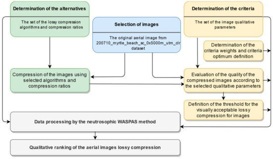
Figure 1.
The framework for rating the lossy compression algorithms and their compression ratios by their qualitative suitability for the aerial images. Different colors present stages related to the data selection, lossy compression (alternatives), lossy compression evaluation by the qualitative parameters (criteria) and data processing for qualitative ranking of lossy compression.
The transform-based lossy compression algorithms—JPEG2000, ECW, and JPEG—were selected to implement our methodology. The algorithms were ranked by the amount of the distortions introduced to the aerial image, estimated using: (a) the supervised objective image quality measures; (b) subjective evaluation; (c) the change in the appropriate first-order statistical measures; (d) the change in the second-order statistical measures. The novelty of the approach is the use of a weighted combination of different qualitative parameters for lossy compression estimation compared to the estimation using only single objective image quality metrics. Thus, the effect of lossy compression on the image content can be evaluated more precisely. This also allows targeting different subtasks, either altering the weights or the set of aspects: the same approach can be used to assess the texture or color quality after the compression.
3.2. Lossy Compression Algorithms for Aerial Images
In this work, three lossy transform-based compression algorithms, namely, JPEG2000 [41], ECW [42,43], and JPEG [44], were selected as alternatives for MCDM methodology to evaluate them by compression efficiency. JPEG2000 is a still image (greyscale, color etc.) encoding and decoding system that defines both lossy and lossless compression techniques based on the discrete wavelet transform (DWT) method [45]. ECW is a proprietary lossy compression format based on the DWT method, targeted for satellite imagery and aerial photography [46]. JPEG is a commonly used image encoding and decoding system, using a lossy compression technique based on the DCT [47].
It has been stated [48] that the transform-based compression is less sensitive to changes in the statistical image properties, and the subjective image quality is preserved better. The proper lossy compression technique uses the image data decomposition to reduce the redundant information and maintain the quality of the image. The generalized scheme for lossy aerial image compression and decompression is presented in Figure 2. It consists of the reduction in redundancy, entropy coding, bit stream transmission, decoding, and data reconstruction. The typical encoder performs color space conversion and image decomposition, transformation, quantization and coding [49,50]. The decoder performs entropy decoding, dequantization, inverse transformation, and inverse color space conversion [49,50].
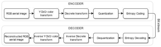
Figure 2.
Basic procedures for aerial image transform-based lossy compression–decompression.
As shown in Figure 1, the encoder converts the original image into the bit stream. The encoded bit stream is received by the decoder, and the restored image is obtained. For the lossy compression system, the total data quantity of the original image is larger than the data quantity of the compressed image. The ratio between these images is called the compression ratio [7,51] and can be expressed as:
where Usize–uncompressed image size; Csize–the size of a compressed image file stored in a disk.
It must be noted that the compression ratio is calculated for the storage size, not the image data, so storing the same compressed image in the different storage formats will affect the compression ratio because of the additional data, introduced by the file format.
The aerial image is transformed from the spatial domain to the frequency domain at the decomposition stage. This process is usually lossless. The JPEG2000 and ECW algorithms use DWT to decompose an image into sub-images (sub-bands) of low-pass (approximate) and high-pass (detail) coefficients at different resolutions. The ECW algorithm exploits this decomposition during compression of images to maintain the quality close to the uncompressed imagery, and the quality at different compression ratios changes less compared to JPEG2000. The difference between JPEG2000 and ECW is the analysis and synthesis filters used for DWT. The JPEG uses a discrete cosine transform (DCT) to obtain the approximation blocks, representing the magnitude of the appropriate frequencies. DWT and DCT coefficients of the decomposed image are ordered by their impact, and coefficients contributing insignificant information to image content may be omitted. Properties like energy compaction, data decorrelation, computational speed characterize the discrete transforms and can be reused in data compression.
The quantization is an irreversible process in the lossy compression pipeline. It is a compromise between the quality of the image and the compression ratio. As the lower frequencies provide the most important part of the information in the image, there is a possibility to discard high-frequency components and reduce the amount of data considering the human eye is almost insensitive to the rapidly varying differences in brightness (high frequencies). In the JPEG pipeline, blocks containing high-frequency and thus low-importance coefficients that are close to zero are discarded to get an enhanced compression rate. The visually weighted quantization tables are exploited for the minimization of the perceptible loss of information. Considering that each sub-band has different importance based on the human perceptibility, the selection of the quantizer step-size can exploit the human visual system (HVS) model like DCT quantization tables in JPEG. The JPEG2000 uses a uniform scalar quantizer to quantize wavelet sub-band coefficients, for which the magnitudes are below the quantizer step-size. The sub-bands of each JPEG2000 image tile are further divided into non-overlapping blocks—the rectangular arrays for entropy coding. Similar to JPEG2000, the ECW quantization is adopted to the coefficients of separate wavelet sub-bands. The image compression is achieved after the quantization.
For the creation of the compressed bit stream, the JPEG2000 algorithm uses Embedded Block Coding with Optimized Truncation (EBCOT) that encompasses the arithmetic coding system. The entropy coder of JPEG uses Huffman coding. The encoded bit stream can be transmitted over communication channels or stored in repositories. The encoding procedure is lossless.
The compressed image is reconstructed via decoding, dequantization, and transformation, inverse DWT for JPEG2000/ECW and inverse DCT for JPEG. Finally, the color transform from YCbCr to the presentation color space is performed. The reconstructed aerial image is a close approximation of the original image, as distortions are introduced during lossy compression.
Since ECW is a proprietary algorithm, only the compression results can expose its peculiarities. The aerial images were compressed by the ECW algorithm using Global Mapper v20.0.1 software package [52] in our work.
3.3. Qualitative Parameters for Compressed Aerial Images
In aerial images, the different areas like grass, sand, vegetation, water, and others may be defined as regions of different textures. As the texture is defined by the local fluctuations of intensities or color brightness in an image, a human can discern the appropriate regions even in grayscale images by distinct textures. The region of rough texture is characterized by contrasting values of the neighboring pixels (e.g., forest canopy). The smooth region contains pixels of similar values (e.g., calm water) [27]. Texture characteristics are used in various application areas of remote sensing images like segmentation and classification [23,53,54]. The aerial images are rich not only in texture but also in color information. This information is used for edge detection, segmentation, classification, and other purposes [5,36,37].
The visual features depend on the image content since it is represented by the spatial arrangement and interrelationships of pixel values. The pixel-based approaches are widely used in change detection in remote sensing data [23,55]. Because of this, it is essential to evaluate the impact of lossy compression on the visual features of the aerial image content. Change detection of the texture and color characteristics can be evaluated by numerical pixel-based statistical measures [20,55]. The image does not require the prior processing to assess the statistical change of information after lossy compression and statistics are calculated for the compressed and the original image to find the differences.
There are different methods to calculate the texture features, like Gabor Filter [56], wavelet [57], Grey Level Co-occurrence Matrix (GLCM) [53,54,55]. The GLCM-based method is commonly used for texture analysis and discrimination using second-order histogram statistics. In [58], the authors proposed 14 statistics properties to describe the texture. There are five commonly used Haralic statistical measures (irrelative to each other) for texture analysis in remote sensing images: contrast, correlation, energy, entropy, and homogeneity [53,59]. The statistical texture measures are calculated using the probability matrix P of the GLCM method. The number of grey levels in the aerial image determines the dimensions of this matrix. The gray levels can be quantized with the cost of the reduction in the information [60]. Each element (i, j) of the probability matrix P defines the frequency of a pixel of the i grayscale intensity occurring at a specified distance d and direction adjacent to a pixel of a grayscale intensity j. Smaller distances are used for capturing local information [54].
In this research, we used five GLCM-based statistics to evaluate the distortions introduced into the grayscale image (Y channel of YCbCr color space) textures after lossy compression: contrast, correlation, homogeneity, energy, entropy.
The contrast [53,54,58] statistic measures the intensity contrast between each image pixel and its neighbor. This statistic presents the local variations in the image content and is defined by the equation:
where P—the probability matrix, —location of the current pixel.
The correlation [53,54,58] shows the link between a pixel and its neighbors. It also reflects texture similarity in the appropriate direction and will be high for the image regions with a linear structure. The correlation is expressed as:
where —the mean, —the standard deviation.
The homogeneity [53,54,58] statistic reflects how close to the GLCM diagonal are distributed the elements of GLCM. Low contrast image exposes high values of homogeneity. This statistic is closely related to the change of the pixel intensity values in the image region. The homogeneity is calculated as:
The energy [53,54,58] statistic measures the uniformity. The less smooth the texture of the image is, the lower its energy value. The energy is computed as:
The entropy [53,54,58] measures the image information. The high entropy reflects the high complexity and disorder of the image textures. The smooth textures have low entropy values. The entropy statistic is computed as:
The effect of lossy compression on the image color is defined by first-order statistics—mean and standard deviation—of Cb and Cr color channels of YCbCr color space in our research. These histogram-based statistics are global as they do not localize image distortions in the spatial domain. The one-dimensional histogram is used to provide statistical information about the greyscale or color image or textures. The probability density function p(i) can be calculated by dividing the values of intensity level histogram h(i) by the number of image pixels [61]:
where —the number of image intensity levels.
The average intensity level of the image is defined by the mean statistics. The standard deviation defines the density of the image intensity dispersion around the mean.
Supervised quality metrics—PSNR, PSNR-HVS-M, SSIM, MS-SSIM—compare the distorted image with reference. We included subjective metrics alongside the commonly used supervised objective metrics to evaluate the quality of lossy aerial image compression.
Simple pixel-based differences metric—Peak Signal to Noise Ratio (PSNR) is usually used for assessment of image distortion after lossy compression. The PSNR is only an approximation to human visual perception. Peak signal to noise ratio between the original and compressed images [62] is calculated as:
where MSE—the mean square error; B—the bits per sample.
The Mean Square Error (MSE) [62]:
where M and N—the width and high of the aerial image, respectively.
For YCbCr color space, PSNR is computed as [62]:
PSNR-HVS-M metric was designed to improve PSNR’s performance [63,64], taking into account the HVS. The original and distorted images are divided into 8 × 8 non-overlapping blocks of pixels. The difference between each distorted and original block of DCT coefficients is multiplied by a contrast masking metric (CM), and further, the result is weighted using coefficients of Contrast Sensitivity Function (CSF) [64]:
Then, the MSE in DCT domain [64]:
where (I, J)—the position of the 8 × 8 non-overlapping block in the image; (i, j)—the position of the pixel in the block.
PSNR-HVS-M is computed using Equation (8) and replacing MSE with . Values of PSNR and PSNR-HVS-M metrics are in the range [0, ] dB.
The Structural Similarity Index (SSIM) [65,66] shows the similarity between the two images—the original and reconstructed after compression. The changes of structural information are analyzed in the images using the structure s, luminance l, and contrast c. This HVS-based metric is usually applied to a luminance channel of images (Y channel of YCbCr color space). For j-th scale SSIM, the quality assessment is defined as [66]:
for j = 1, …, M−1 and
for j = M. In (7) and (8), , are i-th local image patches at the j-th scale that are extracted from i-th evaluation widow, and —the number of the evaluation windows in the scale.
The overall multiscale SSIM is denoted as MS-SSIM [66] and is expressed by the equation:
where —the values that are obtained through psychophysical measurements [56].
The values of SSIM and MS-SSIM metrics are in the range from [0, 1]. High image quality is indicated by the high score of SSIM, MS-SSIM, PSNR, and PSNR-HVS-M.
A subjective evaluation of the distorted image quality is based on human visual perception. This method is called the Mean Opinion Score (MOS) [62] and defines the average score of opinions. MOS is commonly used to assess the image quality in a broad spectrum of applications, including image compression. Human judgment is important, but the subjective method is time-consuming and can fail to evaluate high-resolution images because of the vast amount of the data present; it is almost impossible to perceive and estimate the small distortions. This method is reasonable to combine with objective methods.
These four groups of qualitative parameters are presented in Figure 3.
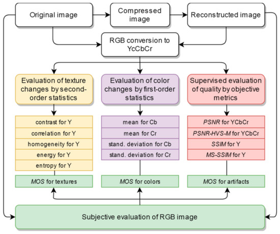
Figure 3.
Qualitative parameters for the evaluation of the reconstructed aerial image after lossy compression. Different colors represent different groups of qualitative parameters.
They were used as criteria for the qualitative evaluation of aerial image lossy compression using MCDM methodology. The chosen combination of the different types of qualitative measurements can improve the qualitative assessment of the image reconstructed after lossy compression.
3.4. Evaluation of the Criteria Weights
One of the constituent parts of MCDM methods is the determination of criteria weights. The criteria weights were assessed using the subjective direct weight determination method. The majority of the present methods for the determination of criteria weights are based on the subjective expert judgment [67,68]. The direct weighting method of criteria importance was used in most cases. This widespread, while subjective, method has higher accuracy compared to the ranking method [68]. Using the criteria weights direct determination method, the sum of all the assessment weights of each expert must be equal to 100% or 1.0 [69,70,71].
The qualitative parameters—criteria—were provided for the experts to evaluate their importance. The calculation of the importance of a criterion is calculated according to (16):
where —the estimation value of i criterion by k expert, and r is the number of experts.
The weights of the criteria are calculated using (17):
where r is the number of experts, m—the number of criteria, —i criterion by expert.
The assessment of the importance of qualitative parameters by experts and the calculated weight of each parameter are presented in Table 1.

Table 1.
Evaluation of the importance of criteria and their weights.
3.5. MCDM WASPAS Method for Data Processing and Evaluation
In the present research, WASPAS has been selected for the exploration of the problem related to the qualitative rating of aerial image lossy compression. The applications of the WASPAS method were presented in [67]. The WASPAS approach is used for the solution to a broad range MCDM problems. This method is popular due to stability and simplicity. WASPAS method initially was introduced in [72] and later was extended by single-valued neutrosophic sets (WASPAS-SVNS) [73]. Although this method has been already used to solve different MCDM tasks [74,75], we could not find any research where WASPAS was applied to assess the lossy compression in the satellite images.
WASPAS-SVNS approach can be decomposed into several steps [73] presented below:
- For the construction of the decision matrix, we need to have the initial information that consists of the evaluations of lossy compression algorithms and compression ratios (as alternatives) according to the qualitative parameters of compressed aerial images (as criteria). When the decision matrix X is constructed, vector normalization is used to normalize the decision matrix X.
Here, , i = 1, …m; j = 1, …n is the value of the of variable for the ithalternative (criteria).
- 2.
- Then, the neutrosophication and calculation of the neutrosophic decision matrix are performed. For the conversion between crisp normalized values and single-valued neutrosophic numbers (SVNNs), is calculated. Elements of the neutrosophic decision matrix are the single-valued neutrosophic numbers , where t is the membership degree, i—the indeterminacy degree and f—the non-membership degree. The standard crisp-to-neutrosophic mapping will be applied in this study.
- 3.
- The first decision component that is based on the sum of the total relative importance of the ith alternative is calculated by the equation:
Here, the values and are associated with the criteria which are maximized; consequently, and correspond to the criteria which are minimized. The weight of criteria is an arbitrary positive real number, the amount of the maximized criteria is , and the amount of the minimized criteria is . For the single-valued neutrosophic numbers (SVNNs), the following algebra operations should be applied:
Here, and .
- 4.
- The second decision component based on the product of total relative importance in the ith alternative is calculated by the equation:
- 5.
- The following equation calculates the weighted criteria:
- 6
- The final ranking of the alternatives is evaluated considering the descending order of the . This is a score function (further referred to as utility function) for deneutrosophication of the joint generalized criteria and is calculated as follows:
4. An MCDM Application for the Selection of Lossy Compression Algorithms and Discussion
In this section, we present the verification of the proposed methodology on the qualitative selection of lossy compression for the aerial images. The aerial images of different content and resolution were selected for the compression and the qualitative evaluation of their lossy compression. The set of qualitative parameters named criteria, encompass the general image quality assessment metrics, first-order color statistics, second-order texture statistics, and subjective evaluation. The influence of the lossy compression algorithms with different compression ratios to the aerial images’ content was estimated using the set of criteria. The compression algorithms with appropriate compression ratios were ranked according to the qualitative degradation for corresponding compressed image using the neutrosophic WASPAS-SVNS method.
4.1. Compression of Aerial Images
Three lossy compression algorithms were selected for the initial experiment: JPEG200, ECW, JPEG. As the quality of the compressed image depends not only on the compression algorithm but also on the compression ratio, four compression ratios were selected for each algorithm named as follows: low (25:1), medium (50:1), high (75:1), very high (100:1). The influence of the compression ratios lower than 25:1 is negligible, as shown in [19,31,34]. Higher compression ratios deteriorated image quality significantly and were not estimated in this work. Larger intervals between compression ratios were chosen to make their effect on the content of an image more explicit. Each algorithm introduces unique artifacts to the image content that are more noticeable in the higher compression ratios.
The GLOBAL MAPPER software [46] was used for the ECW compression of the original aerial images. The RGB color *.tiff image file saved as the *.ecw image using Global Mapper changing the compression ratios. The imwrite() function from MATLAB was used for JPEG2000 and JPEG compression. The source images were obtained as TIFF images with lossless compression. The JPEG2000 compressed files were generated using the imwrite(…, “CompressionRatio”, Value) function, altering Value for the target compression ratio. For JPEG compression imwrite(…, “Quality”, Value) function was used, altering Value as the quality from 100 to 1 of the JPEG compressed file. The smaller the number, the more compression will be reached with the worse quality for the image. All other settings for the imwrite() function were set to default values. The experimental compression ratios were tailored and verified using Equation (1).
The content and resolution of the image also affect the result of the lossy compressed image. Relevant compression algorithms have different effects on image textures, colors, and luminance. Three high-resolution (1 pixel = 0.5 m) aerial images of different content were selected using Earth Explorer [76]. The aerial images used in the experiment (Figure 4) are “img1”, “img2”, and “img3” of the dataset 200710_myrtle_beach_sc_0x5000m_utm_clr, saved as 3000 × 3000 24-bit TIFF images in RGB (8 bits for each band). The “img1” has more smooth textures with low spatial frequencies of intensity changes, and the large regions of different colors and intensities dominate in it. The “img2” is rich with similar rough textures with high spatial frequencies of intensity changes, and small regions occupy a slight part of the image. The “img3” has various types of textures, and a large number of regions differ in size, color, and intensity [27]. We have tested other images with similar textures and colors to verify objective qualitative parameters. Images were selected by the varying characteristic features (texture, color tone, luminance, number, and size of the objects) but not by the appropriate classes, as the aim is to verify the methodology.
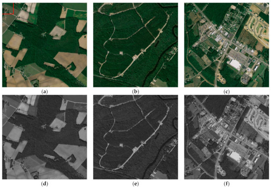
Figure 4.
The original aerial images used in the experiment (Landsat-7 images courtesy of the U.S. Geological Survey): (a) “img1” in RGB. The red rectangular indicates a cropped region presented in Figure 5); (b) “img2” in RGB; (c) “img3” in RGB; dataset 200710_myrtle_beach_sc_0x5000m_utm_clr. (d) “img1”, component Y; (e) “img2”, component Y; (f) “img3”, component Y.
For the other three images of different resolutions, the original images were reduced four times using the impyramid() MATLAB function. The reduced “img1”, “img2”, and “img3” will be referenced as “img4”, “img5”, and “img6” accordingly, with the resolution of 1 pixel = 2 m and the size of 750 × 750 pixels. The remote sensing images with higher spatial resolution have richer spatial textures as their pixels contain more information compared to low-resolution images. All six images of different structures were compressed using three different algorithms using four compression ratios. Figure 5 presents the cropped images “img1” and “img4” compressed using JPEG2000, ECW, and JPEG algorithms at a 100:1 compression ratio.
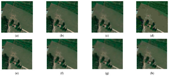
Figure 5.
The same cropped region of the aerial images “img1” and “img4” compressed using different lossy compression algorithms at the compression ratio 100:1: (a) “img1”, the original image; (b) “img1”, Joint Photographic Experts Group (JPEG)2000 compression; (c) “img1”, Enhanced Compression Wavelet (ECW) compression; (d) “img1”, JPEG compression; (e) “img4”, the reduced “img1”; (f) “img4”, JPEG2000 compression; (g) “img4”, ECW compression; (h) “img4”, JPEG compression.
4.2. Qualitative Evaluation of Aerial Image Lossy Compression
The qualitative evaluation was performed using MATLAB. After lossy compression of images “img1”, “img2”, “img3”, “img4”, “img5”, and “img6” all selected qualitative parameters were calculated and estimated using the original and reconstructed versions of the aerial images.
The first group of parameters—texture change of images after compression—includes the second-order statistics: contrast (Equation (2)), correlation (Equation (3)), homogeneity (Equation (4)), energy (Equation (5)), and entropy (Equation (6)). The GLCM-based statistics were calculated for the luminance component in the YCbCr space of the original and compressed images. The difference between them was used to evaluate texture changes. The size of the probability matrix P of the GLCM method was determined by the number of the original gray levels in the Y component. The smaller distances between the image pixel of interest and its neighboring pixel are used to capture local texture information. For 3000 × 3000 images with the resolution of 1 pixel = 0.5 m and for 750 × 750 images with resolution of 1 pixel = 2 m were taken different displacements (respectively, d = 1, 2, 3, 4, 5, 6, and d = 1) for six directions ( = 0°, 45°, 90°, 135°, 180°, 225°, 270°and 315°) as the texture changes are to be assessed in the same area. The extra pixel in each direction is used to minimize the influence of pixel-shifting during image resizing. The mean of each GLCM’s texture statistic was calculated to define final contrast, correlation, homogeneity, energy, and entropy measures used to evaluate changes after lossy compression. Calculated texture changes between the original and compressed images are presented in Figure 6a–e. The more significant difference between the qualitative parameters of textures of the original and distorted images, the higher impact of lossy compression was on the loss of image texture information. As seen from Figure 6a,e, changes of texture contrast and entropy commonly increase with increasing compression ratios for the selected algorithms. However, statistical changes in textures increase in the negative direction for correlation, homogeneity, and energy as the compression ratios increase (Figure 6b–d). Table 2 in the first five rows shows the same results for the calculated qualitative texture parameters, respectively, C1, C2, C3, C4, and C5 but only for the “img1”. The differences between the qualitative parameters of textures of the original and distorted images slightly decrease in some cases from the lower compression ratios to the higher as presented in Figure 6c,e, respectively, for homogeneity and entropy changes using ECW lossy compression from 75:1 to 100:1 compression ratios for “img5”.
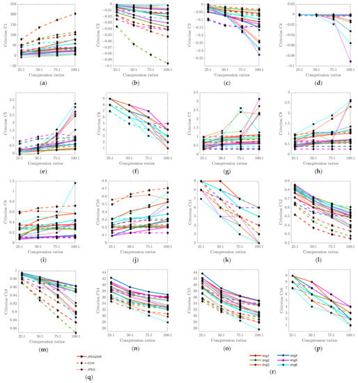
Figure 6.
Influence of lossy compression with selected compression ratios to the quality of the reconstructed different aerial images after compression. Distinct colors represent aerial images “img1”, “img2”, “img3”, “img4”, “img5” and “img6”. Different line types represent lossy compression algorithms JPEG2000, ECW, JPEG. Each figure shows the results of the selected qualitative parameter (criterion) for the six images compressed with different algorithms: (a) C1—contrast change for Y component; (b) C2—correlation change for Y component; (c) C3—homogeneity change for Y component; (d) C4—energy change for Y component; (e) C5—entropy change for Y component; (f) C6—MOS for RGB image texture; (g) C7—change of the mean of Cb component; (h) C8—change of the mean of Cr component; (i) C9—change of the standard deviation of Cb component; (j) C10—change of the standard deviation of Cr component; (k) C11—MOS for RGB image colors; (l) C12—SSIM for Y component; (m) C13—MS-SSIM for Y component; (n) C14—PSNR for YCbCr image; (o) C15—PSNR-HVS-M for YCbCr image; (p) C16—MOS for RGB image artifacts; (q) legends for marking the separate algorithms in each figure; (r) legends for marking the separate images in each figure.
Table 2.
Impact of the lossy compression algorithms with relevant compression ratios to the aerial image “img1” content.
The second group of parameters—color change of images after compression—includes the first-order statistics: mean and standard deviation of Cb and Cr components. Calculated color changes between the original and the compressed images are presented in Figure 6g,h,i,j. The more significant the difference between the original and distorted images’ qualitative color parameters, the higher the impact of lossy compression on the distortions of color information. Changes of chrominance (mean and standard deviation) commonly increase with increasing compression ratios for the selected algorithms. Rows from 7 to 10 in Table 2 show the calculated results of the qualitative texture parameters C7, C8, C9, and C10 for the “img1”. For JPEG lossy compression ratios from 75:1 to 100:1, the change of the mean for the Cb component considerably decreases for “img6”, as presented in Figure 6g.
The third group of parameters—supervised objective IQA metrics—includes PSNR for YCbCr image (Equation (8)), PSNR-HVS-M for YCbCr image (Equation (10)), SSIM for Y component (Equations (13) and (14)), MS-SSIM for Y component (Equation (15)). The supervised objective quality metrics compare the compressed images with the original, and the better image quality is indicated by a higher score (Figure 6l–o). The same results of IQA metrics for the “img1” are presented in Table 2, rows 12 to 15, respectively, including criteria C12, C13, C14, and C15. IQA metrics decrease with increasing compression ratios for the selected algorithms for all images.
The fourth group of parameters—subjective evaluations of RGB images after compression—includes MOS values in the range from 1 to 10 using a 10-point Likert scale [77] for the quality of image textures, colors, and artifacts after compression. The meaning of the qualitative parameters C6, C11, C16, and a rating scale was explained to the 15 students of Information Technologies. They were provided with a questionnaire (see Appendix A) and an individual blank response table (Table 2), excluding all rows except the sixth, eleventh, and sixteenth. The respondents were asked to fill the response tables for the six images. The assessments’ mean values were calculated and included as criteria C6, C11, and C16. Estimated MOS values for textures, colors, general artifacts after lossy compression are presented in both Table 2 and Figure 6f,k,p.
The threshold for the acceptable visible distortions in aerial images reconstructed after each lossy compression was estimated visually by five experts from Vilnius Gediminas technical university, Department of Graphical systems with at least 15 years of experience in image processing. These experts also present their opinion concerning the image visual criteria weights considered in Section 3.4. The qualitative parameters from acceptable compression ratios for each algorithm and image were taken considering their groups—texture, color, IQA. Three threshold alternatives—JPEG2000-A01, ECW-A02, JPEG-A03—were constructed to evaluate acceptable visible distortions for each algorithm (Table 2, A13, A14, A15). The threshold alternatives help to decide at which compression ratios of selected lossy compression algorithms are aerial images’ distortions visually acceptable.
4.3. Ranking of Aerial Image Lossy Compression
After the alternatives were defined and qualitative criteria were calculated, the initial decision matrix for qualitative evaluation of the lossy compression of aerial images was formed. The example of the initial decision matrix for “img1” is presented in Table 2. As the matrix has negative values for the change of correlation, homogeneity, and energy, to make calculations consistent with WASPAS-SVNS, the rows with negative values were upshifted before the vector normalization. The obtained results by WASPAS-SVNS methodology described in Section 3.5 (steps 2–6) are presented in Table 3. The qualitative ranking of images’ lossy compression was calculated using the utility function (Equation (27)). Figure 7 presents the ranking of lossy compression for high and low-resolution images. Ranking of compression algorithms based on their qualitative suitability for the images makes it difficult to decide which compression ratios of lossy compression are unacceptable for visual inspection. Qualitative ranking by estimating the threshold of acceptable visual distortions places the algorithms with their compression ratios in order of priority, excluding those whose distortions are greater than the subjectively determined quality threshold (Table 3, Figure 8).
Table 3.
Qualitative ranking of aerial images’ lossy compression.
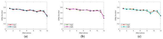
Figure 7.
Qualitative ranking of the high- and low-resolution aerial images’ lossy compression using the selected alternatives as 1 (A1)—JPEG2000, 25:1; 2 (A2)—ECW, 25:1; 3 (A3)—JPEG, 25:1; 4 (A4)—JPEG2000, 50:1; 5 (A5)—ECW, 50:1; 6 (A6)—JPEG, 50:1; 7 (A7)—JPEG2000, 75:1; 8 (A8)—ECW, 75:1; 9 (A9)—JPEG, 75:1; 10 (A10)—JPEG2000, 100:1; 11 (A11)—ECW, 100:1; 12 (A12)—JPEG, 100:1: (a) “img1” and its reduced version “img4”; (b) “img2” and its reduced version “img5”; (c) “img3” and its reduced version “img6”.
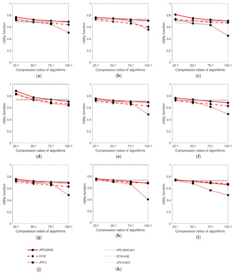
Figure 8.
Qualitative ranking of lossy compression algorithms with selected compression ratios solving the full and partial tasks for aerial images: (a) “img1”—by all the selected qualitative parameters (b) “img1”—by the texture quality; (c) “img1”—by the color quality; (d) “img1”—by the general quality metrics; (e) “img2”—by the all selected qualitative parameters; (f) “img3”—by the all selected qualitative parameters; (g) “img4”—by the all selected qualitative parameters; (h) “img5”—by the all selected qualitative parameters; (i) “img6”—by the all selected qualitative parameters; (j) legends for marking the compression algorithms for each image; (k) legends for marking the thresholds of compression quality of separate algorithms for each image.
As presented in Table 3 and Figure 7a–c graphs, the ranking of algorithms with different compression ratios according to the qualitative suitability for the high-resolution images “img1” and “img2” do not coincide. The “img3” ranking differs more from the first two because its content has more features sensitive to the lossy compression, such as the different types of textures, many small regions of different colors and intensities. The best quality presents JPEG2000 25:1 compression for all high-resolution images (1st place in Table 3, row 1), and the worst—JPEG 100:1 (15th place in Table 3, row 12). The JPEG2000 algorithm maintains better image quality than ECW and JPEG at compression ratios 50:1, 75:1, 100:1 (Table 3, JPEG2000 alternatives at 1st, 4th, 7th, 10th rows) too. Considering the threshold alternative A13 for the JPEG2000 algorithm (Table 3, 13th row), a visually acceptable lossy compression for “img1” and “img2” was ranked above 6th place and for “img3” above 7th place. This corresponds to JPEG2000 compression lower than 100:1 for “img1” (Figure 8a) and lower than 75:1 for “img2” and “img3” (Figure 8e,f). ECW and JPEG algorithms were ranked worse than JPE2000 at all compression ratios. At lower compression ratios 25:1, 50:1, the JPEG algorithm (Table 3, JPEG alternatives at 3rd, 6th rows) was ranked higher than the ECW algorithm for “img1” and “img2”. However, for “img3” can be seen the opposite tendency. At higher compression ratios 75:1, 100:1, the JPEG algorithm (Table 3, JPEG alternatives at 9th, 12th rows) was ranked worse than the ECW algorithm for “img1” and “img3”. For “img2”, JPEG 75:1 was ranked higher than ECW 75:1. Considering the threshold alternative A15 for the JPEG algorithm (Table 3, 15th row), a visually acceptable lossy compression for “img1” was ranked above 9th place, for “img2” above 3rd place, and for “img3” above 6th place. This corresponds to JPEG compression lower than 75:1 for “img1” (near to 50:1 and less, Figure 8a), lower than 50:1 for “img2” and “img3” (near to 25:1 and less Figure 8e,f). The ECW compression rating is presented in 2nd, 5th, 8th, 11th rows of Table 3. At lower compression ratios 25:1, 50:1, the ECW algorithm was rated worse than the JPEG algorithm for “img1” and “img2”, but at very high—100:1—compression ratios was rated higher than JPEG2000. Considering the threshold alternative A14 for the ECW algorithm (Table 3, 14th row), a visually acceptable lossy compression for “img1” was ranked above 11th place, for “img2” above 12th place, and for “img3” above 3rd place. This corresponds to ECW compression lower than 75:1 for “img1” (near to 50:1 and less, Figure 8a), and lower than 50:1 for “img2” and “img3” (near to 25:1 and less, Figure 8e,f).
A similar ranking tendency is observed for the corresponding low-resolution images “img4”, “img5”, and “img6” (Figure 8), but the changes of images’ content due to the reduced resolution made the influence on the rating of lossy compression. The best quality presents JPEG2000 25:1 compression for all low-resolution images (1st place–Table 3, row 1), and the worst—JPEG 100:1 (15th place—Table 3, row 12). The JPEG2000 algorithm maintains better quality than ECW and JPEG at compression ratios 50:1 and 75:1 for “img4” and “img5”, but at 100:1 for “img5” is superior ECW compression (Table 3, JPEG2000 alternatives at 4th, 7th, 10th rows). ECW compression at compression ratios 50:1, 75:1, 100:1 is superior to JPEG2000 compression for “img6” too. Considering the threshold alternative A13 for the JPEG2000 algorithm, a visually acceptable lossy compression for “img4” was ranked above 7th place, for “img5” above 4th place, and “img6” above 6th place. This corresponds to JPEG2000 compression lower than 75:1 for “img4” and “img5” (near to 50:1 and less, Figure 8g,h), and lower than 50:1 for “img6”. At higher compression ratios 75:1, 100:1, the ECW algorithm was ranked higher than the JPEG for the selected low-resolution images, but at low—25:1—compression ratios was ranked worse than JPEG for “img4” and “img5”. Considering the threshold alternative A14 for the ECW algorithm, a visually acceptable lossy compression for “img4” was ranked above 4th place, for “img5” above 9th place, and “img6” above 3rd place. This corresponds to ECW compression lower than 50:1 for “img4”, “img5,” and “img6” (near to 25:1 and less, Figure 8g–i). A visually acceptable JPEG lossy compression for was ranked by A15 alternative for “img4” above 5th place, for “img5” above 6th place, and “img6” above 5th place. This corresponds to JPEG compression lower than 50:1 for “img4”, “img5,” and “img6” (for all images near to 25:1 and less, Figure 8g–i).
The effect of lossy compression on the image content can be evaluated more precisely by the set of qualitative parameters and by using the parameters of the texture, color, and IQA, different subtasks can be solved: the same approach can be used to assess the texture, color, and general quality after the image lossy compression. Figure 8 shows the qualitative suitability of JPEG2000, ECW, JPEG compression for “img1” solving the full (Figure 8a,e–i) and partial tasks (Figure 8b–d)). Figure 8 shows that the JPEG2000 lossy compression is superior to the lossy ECW and JPEG compression in texture (b), color features (c), and by IQA (d). The JPEG compression provides similar image quality to JPEG2000 in texture features only at low compression ratios. JPEG has a significant effect on color, except at low compression ratios. The ECW compression at high compression ratios negatively affects texture but has a low impact on color. By IQA, the JPEG and ECW compression have a similar effect on the “img1” content.
4.4. Discussion
The ranking of JPEG2000, JPEG and ECW algorithms with different compression ratios differs slightly according to the qualitative suitability for the high-resolution aerial images “img1”, and “img2” (Table 3, Figure 7a,b) as both images have similar features of the content. The “img1” and “img2” have textures of the same RGB values and intensities, but rough textures dominate in the “img2”, while smooth ones are more common in the “img1”. Due to prevalence of rough textures, “img1” has the lower visually acceptable threshold of JPEG2000, JPEG and ECW lossy compression (Figure 8a) and the compression artifacts are barely visible in the compressed image, compared to other ones. The “img3” ranking, as well as the content, differs considerably comparing to the “img1” and “img2” (Table 3, Figure 7c). The “img3” contains more features, sensitive to the lossy compression, like textures with the high spatial frequencies (of intensity change) and a large number of small regions differing in size, color, and intensity.
The changes of the content in the images “img4”, “img5”, and “img6” due to the down sampling also influenced the ranking of lossy compression (Table 3, Figure 7a–c) and the visually acceptable threshold of lossy compression (Figure 8g–i). The low-resolution aerial images do not have the rich spatial textures of the high-resolution images, and their lossy compression artifacts are more noticeable. The “img6” has the highest visually acceptable threshold of JPEG2000, JPEG and ECW lossy compression (Figure 8i) compared to “img4” and “img5” (Figure 8g,h). After the image “img2” was down sampled to the “img5”, the textured regions became smoother. As the textures in the “img1” are of dominating low spatial frequencies of intensity changes, then down sampling it to the “img4” exposes a smaller effect on the visual content of the image. Thus, the low-resolution images “img4” and “img5” were similarly affected by lossy compression, especially at higher compression ratios for JPEG (Figure 8g,h).
Each algorithm introduces unique artifacts and has a different effect on the aerial images of different resolutions and contents. The JPEG lossy compression has a high impact on the images’ content with uniform and coarse (low spatial frequencies of intensity changes) textures. The “img1” and “img3” contains this type of textures, but “img3” was affected more by JPEG compression as it contains a large number of small, uniform regions. The JPEG2000 compression more affects images containing a large number of regions with textures of high spatial frequencies of intensity changes (“img2”), and especially with the small regions of different textures (“img3”). The ECW lossy compression has a higher effect on images rich with rough textures of high spatial frequencies of intensity changes (“img2”). The JPEG2000 and ECW compression have a similar effect for low-resolution images with textures of high spatial frequencies of intensity changes (“img5”), or with small regions with different textures (“img6”). The JPEG2000 has higher quality at higher compression ratios than JPEG as it does not expose visually distracting artifacts, especially in low frequency or uniform areas. The JPEG artifacts are more pronounced in the low-resolution images’ content than they are in the high-resolution images. The smoothing artifacts are more noticeable in ECW high-resolution images than in JPEG2000, specifically in images with textures of high spatial frequencies of intensity changes. The ECW compression has a slightly lesser effect on the low-resolution images.
5. Conclusions and Future Work
We proposed the original multi-criteria decision-making methodology for the qualitative selection of the lossy compression for the aerial images based on their resolution and content. The transform-based lossy compression algorithms with the appropriate compression ratios were ranked by their suitability for aerial images using MCDM WASPAS-SVNS and direct criteria weights evaluation methods. The rating of lossy compression is governed by the set of qualitative parameters of images and visually acceptable lossy compression ratios.
Because of the need for the qualitative lossy compression for the effective storage and transmission of a large amount of remote sensing data, it is imperative to decide which algorithm and what compression ratio will be suitable for the selected image content and resolution. Since the image quality after lossy compression can be determined by various parameters, and they belong to the different groups that vary significantly, the weighted combination of different qualitative parameters should be used.
The visual features (e.g., a forest, cropland, roads, buildings, water) in an image can be characterized by generalizations like texture, color tone, and luminance. The information on the change of the colors and textures can be calculated using the first-order color statistics and second-order texture statistics, respectively. It is reasonable to include the often-used objective IQA metrics and subjective evaluation. Using the set of the verified groups of parameters and altering their weights, the effect of lossy compression on the image content can be evaluated more precisely compared to the estimation using only single objective image quality metrics.
The use of the set of the qualitative parameters for the texture, color, and IQA, can solve different subtasks: the same approach can be used to assess the texture, color, and general quality after the image lossy compression.
In the aerial imagery application context, it is useful to define the acceptable lossy compression ratio for the selected lossy compression algorithm. We concentrated on visual image inspection after data collection and compression for easier transmission and saving storage space. It should be useful to find the best solution for image lossy compression implementation in hardware in such cases. The threshold of acceptable visual distortions places the algorithms with their compression ratios in order of priority, excluding those whose distortions are greater than the subjectively determined quality threshold. The experimental results showed that the visually acceptable lossy compression for the high-resolution aerial images is: JPEG2000—lower than 100:1 for “img1” and lower than 75:1 for “img2” and “img3”; ECW and JPEG—lower than 75:1 for “img1” (near to 50:1 and less), lower than 50:1 for “img2” and “img3” (near to 25:1 and less). The visually acceptable lossy compression for the low-resolution aerial images is worse than for the high-resolution images: JPEG2000—lower than 75:1 for “img4” and “img5” (near to 50:1 and less), and lower than 50:1 for “img6”; ECW and JPEG—lower than 50:1 for “img4”, “img5,” and “img6” (near to 25:1 and less).
As the lossy compression quality is a complex task and needs to be investigated further, we are going to evaluate the lossy compression quality for the different classes of satellite images against the segmentation using the appropriate set of qualitative parameters.
Author Contributions
Conceptualization, R.B. and G.K.-J.; methodology, R.B., G.K.-J.; software, G.K.-J.; validation, R.B., G.K.-J.; formal analysis, R.B., G.K.-J.; investigation, G.K.-J.; resources, R.B., G.K.-J.; data curation, G.K.-J.; writing—original draft preparation, G.K.-J.; writing—review and editing, R.B., G.K.-J.; supervision, R.B; project administration, R.B. All authors have read and agreed to the published version of the manuscript.
Funding
The research received no external funding.
Institutional Review Board Statement
Not applicable.
Informed Consent Statement
Not applicable.
Data Availability Statement
Data sharing not applicable.
Conflicts of Interest
The authors declare no conflict of interest.
Appendix A
The questionnaire for the evaluation of the visual image quality after the relevant lossy compression:
- Evaluate the visual quality of compressed image textures according to the original image textures.
- Evaluate the visual quality of compressed image colors according to the original image colors.
- Evaluate a number of artifacts in the compressed image according to the original image.
References
- ESA. Sentinel-2 User Handbook; ESA: Auckland, New Zealand, 2015; pp. 1–64. [Google Scholar]
- Alam, A.; Bhat, M.S.; Maheen, M. Using Landsat satellite data for assessing the land use and land cover change in Kashmir valley. GeoJournal 2019. [Google Scholar] [CrossRef]
- Fonji, S.F.; Taff, G.N. Using satellite data to monitor land-use land-cover change in North-eastern Latvia. SpringerPlus 2014, 3. [Google Scholar] [CrossRef] [PubMed]
- Tan, K.; Zhang, Y.; Wang, X.; Chen, Y. Object-Based Change Detection Using Multiple Classifiers and Multi-Scale Uncertainty Analysis. Remote Sens. 2019, 11. [Google Scholar] [CrossRef]
- Falco, N.; Mura, M.D.; Bovolo, F.; Benediktsson, J.A.; Bruzzone, L. Change Detection in VHR Images Based on Morphological Attribute Profiles. IEEE Geosci. Remote Sens. Lett. 2013. [Google Scholar] [CrossRef]
- Debusscher, B.; Coillie, F. Object-Based Flood Analysis Using a Graph-Based Representation. Remote Sens. 2019, 11, 1883. [Google Scholar] [CrossRef]
- Hussain, A.J.; Al-Fayadh, A.; Radi, N. Image compression techniques: A survey in lossless and lossy algorithms. Neurocomputing 2018, 300, 44–69. [Google Scholar] [CrossRef]
- Faria, L.N.; Fonseca, L.M.G.; Costa, M.H.M. Performance Evaluation of Data Compression Systems Applied to Satellite Imagery. J. Electr. Comput. Eng. 2012, 2012. [Google Scholar] [CrossRef]
- Hagag, A.; Fan, X.; El-Samie, F.E.A. Lossy compression of satellite images with low impact on vegetation features. Multidimens. Syst. Signal Proces. 2016, 28, 1717–1736. [Google Scholar] [CrossRef]
- Christophe, E.; Thiebaut, C.; Latry, C. Compression Specification for Efficient Use of High Resolution Satellite data. Int. Arch. Photogramm. Remote Sens. Spat. Inf. Sci. 2008, XXXVII, B4. [Google Scholar]
- Hagag, A.; Hassan, E.S.; Amin, M.; El-Samie, F.E.A.; Fana, X. Satellite multispectral image compression based on removing sub-bands. Optik 2017, 131, 1023–1035. [Google Scholar] [CrossRef]
- Ahujaa, S.L.; Bindub, M.H. High Resolution Satellite Image Compression using DCT and EZW. In Proceedings of the International Conference on Sustainable Computing in Science, Technology & Management, Jaipur, India, 26–28 January 2019. [Google Scholar] [CrossRef]
- Indradjad, A.; Nasution, A.S.; Gunawan, H.; Widipaminto, A. A comparison of Satellite Image Compression methods in the Wavelet Domain. IOP Conf. Ser. Earth Environ. Sci. 2019, 280, 012031. [Google Scholar] [CrossRef]
- Genitha, C.H.; Rajesh, R.K. A Technique for Multi-Spectral Satellite Image Compression Using EZW Algorithm. In Proceedings of the International Conference on Control, Instrumentation, Communication and Computational Technologies, Kumaracoil, India, 16–17 December 2016. [Google Scholar] [CrossRef]
- Fiorucci, F.; Baruffa, G.; Frescura, F. Objective and subjective quality assessment between JPEG XR with overlap and JPEG 2000. J. Vis. Commun. Image Represent. 2012, 23, 835–844. [Google Scholar] [CrossRef]
- Manthey, K. A New Real-Time Architecture for Image Compression Onboard Satellites based on CCSDS Image Data Compression. In Proceedings of the 4th International Conference on On-Board Payload Data Compression Workshop, Venice, Italy, 23–24 October 2014. [Google Scholar]
- Kiely, A.B.; Klimesh, M. The ICER Progressive Wavelet Image Compressor. Interplanetary Network Progress Report; California Institute of Technology: Pasadena, CA, USA, 2003. [Google Scholar]
- Bateson, L.; Mcintosh, R. An Investigation into File Formats for the use and Delivery of Large Format Images; British Geological Survey Internal Report; British Geological Survey: Nottingham, UK, 2004. [Google Scholar]
- Simone, F.; Ticca, D.; Dufaux, F.; Ansorge, M.; Ebrahimi, T. A comparative study of color image compression standards using perceptually driven quality metrics. In Proceedings of the Conference on Applications of Digital Image Processing, San Diego, CA, USA, 10–14 August 2008; Volume XXXI, p. 7073. [Google Scholar] [CrossRef]
- Matsuoka, R.; Sone, M.; Fukue, K.; Cho, K.; Shimoda, H. Quantitative analysis of image quality of lossy compression images. In Proceedings of the ISPRS Congress, Istanbul, Turkey, 12–26 July 2004. [Google Scholar]
- Tao, D.; Di, S.; Guo, H.; Chen, Z.; Cappello, F. Z-checker: A framework for assessing lossy compression of scientific data. Int. J. High Perform. Comput. Appl. 2017, 1–19. [Google Scholar] [CrossRef]
- Johnson, B.A.; Jozdani, S.E. Identifying Generalizable Image Segmentation Parameters for Urban Land Cover Mapping through Meta-Analysis and Regression Tree Modeling. Remote Sens. 2018, 10, 73. [Google Scholar] [CrossRef]
- Kupidura, P. The Comparison of Different Methods of Texture Analysis for Their Efficacy for Land Use Classification in Satellite Imagery. Remote Sens. 2019, 11, 1233. [Google Scholar] [CrossRef]
- Sirmaçek, B.; Ünsalan, C. Road Detection from Remotely Sensed Images Using Color Features. In Proceedings of the 5th International Conference on Recent Advances in Space Technologies—RAST2011, Istanbul, Turkey, 9–11 June 2011. [Google Scholar] [CrossRef]
- Kazakeviciute-Januskeviciene, G.; Janusonis, E.; Bausys, R.; Limba, T.; Kiskis, M. Assessment of the Segmentation of RGB Remote Sensing Images: A Subjective Approach. Remote Sens. 2020, 12, 4152. [Google Scholar] [CrossRef]
- Fynn, I.E.M.; Campbell, J. Forest Fragmentation Analysis from Multiple Imaging Formats. J. Landsc. Ecol. 2019, 12. [Google Scholar] [CrossRef]
- Bausys, R.; Kazakeviciute-Januskeviciene, G.; Cavallaro, F.; Usovaite, A. Algorithm Selection for Edge Detection in Satellite Images by Neutrosophic WASPAS Method. Sustainability 2020, 12, 548. [Google Scholar] [CrossRef]
- Öztürk, E.; Mesut, A. Entropy Based Estimation Algorithm Using Split Images to Increase Compression Ratio. Trakya Univ. J. Eng. Sci. 2017, 18, 31–41. [Google Scholar]
- Cheon, M.; Lee, J.S. Ambiguity-based evaluation of objective quality metrics for image compression. In Proceedings of the Eighth International Conference on Quality of Multimedia Experience, Lisbon, Portugal, 6–8 June 2016. [Google Scholar] [CrossRef]
- Hagara, M.; Ondráček, O.; Kubinec, P.; Stojanović, R. Detecting edges with sub-pixel precision in JPEG images. In Proceedings of the 27th International Conference Radioelektronika, Brno, Czech Republic, 19–20 April 2017. [Google Scholar] [CrossRef]
- Zabala, A.; Cea, C.; Pons, X. Segmentation and thematic classification of color orthophotos over non-compressed and JPEG 2000 compressed images. Int. J. Appl. Earth Observ. Geoinf. 2012, 15, 92–104. [Google Scholar] [CrossRef]
- Ales, M.; Kokalj, Z.; Ostir, K. The Effect of Lossy Image Compression on Object Based Image Classification—WORLDVIEW-2 Case Study. Int. Arch. Photogramm. Remote Sens. Spat. Inf. Sci. 2012, 3819, 187–192. [Google Scholar] [CrossRef]
- Elkholy, M.; Hosny, M.M.; El-Habrouk, H.M.F. Studying the effect of lossy compression and image fusion on image classification. Alexandria Eng. J. 2019, 58, 143–149. [Google Scholar] [CrossRef]
- Hayati, A.K.; Dyatmika, H.S. The Effect of JPEG2000 Compression on Remote Sensing Data of Different Spatial Resolutions. Int. J. Remote Sens. Earth Sci. 2017, 2, 111–118. [Google Scholar] [CrossRef][Green Version]
- Ham, Y.; Han, K.; Lin, J.; Golparvar-Fard, M. Visual monitoring of civil infrastructure systems via camera-equipped Unmanned Aerial Vehicles (UAVs): A review of related works. Vis. Eng. 2016, 4. [Google Scholar] [CrossRef]
- Li, R.; Han, D.; Dezert, J.; Yang, Y. A novel edge detector for color images based on MCDM with evidential reasoning. In Proceedings of the 2017 20th International Conference on Information Fusion, Xi’an, China, 10–13 July 2017. [Google Scholar]
- Khelifi, L.; Mignotte, M. A Multi-Objective Approach Based on TOPSIS to Solve the Image Segmentation Combination Problem. In Proceedings of the 2016 23rd International Conference on Pattern Recognition, Cancun, Mexico, 4–8 December 2016. [Google Scholar] [CrossRef]
- Stojčić, M.; Zavadskas, E.K.; Pamučar, D.; Stević, Ž; Mardani, A. Application of MCDM Methods in Sustainability Engineering: A Literature Review 2008–2018. Symmetry 2019, 11, 350. [Google Scholar] [CrossRef]
- Wang, W.M.; Peng, H.H. A Fuzzy Multi-Criteria Evaluation Framework for Urban Sustainable Development. Mathematics 2020, 8, 330. [Google Scholar] [CrossRef]
- Guitouni, A.; Martel, J.-M. Tentative guidelines to help choosing an appropriate MCDA method. Eur. J. Oper. Res. 1998, 109, 501–521. [Google Scholar] [CrossRef]
- Skodras, A.; Christopoulos, C.; Ebrahimi, T. The JPEG 2000 still image compression standard. IEEE Signal Process. Mag. 2001, 18, 36–58. [Google Scholar] [CrossRef]
- Ueffing, C. Wavelet Based ECW Image Compression. Photogrammetric Week 01; Wichmann Verlag: Heidelberg, Germany, 2001. [Google Scholar]
- Mallat, S.A. Wavelet Tour of Signal Processing, 3rd ed.; Academic Press: Cambridge, MA, USA, 2009. [Google Scholar]
- Wallace, G.K. The JPEG Still Picture Compression Standard. Commun. ACM 1991, 34, 31–44. [Google Scholar] [CrossRef]
- Overview of JPEG. 2000. Available online: https://jpeg.org/jpeg2000/ (accessed on 21 January 2021).
- Compression White Paper. Using and Distributing ECW V2.0 Wavelet Compressed Imagery; Earth Resource Mapping Pty Ltd.: Perth, Australia, 2012; pp. 2–27.
- Overview of JPEG. Available online: https://jpeg.org/jpeg/index.html (accessed on 21 January 2021).
- Sonka, M.; Hlavac, V.; Boyle, R. Image Processing, Analysis, and Machine Vision, 4th ed.; Cengage Learning: Boston, MA, USA, 2014. [Google Scholar]
- Gonzalea, R.C.; Woods, R.E. Digital Image Processing, 2nd ed.; Prentice Hall: Upper Saddle River, NJ, USA, 2004. [Google Scholar]
- Hilles, S.M.S.; Hossain, M.A. Classification on Image Compression Methods: Review Paper. Int. J. Data Sci. Res. 2018, 1, 1–7. [Google Scholar]
- Lam, K.W.; Li, Z.; Yuan, X. Effects of Jpeg Compression on the Accuracy of Digital Terrain Models Automatically Derived from Digital Aerial Images. Photogramm. Rec. 2001, 17. [Google Scholar] [CrossRef]
- Blue Marble Geographics. Available online: https://www.bluemarblegeo.com/products/global-mapper.php (accessed on 8 June 2020).
- Dawwd, S. GLCM Based Parallel Texture Segmentation using A Multicore Processor. Int. Arab J. Inf. Technol. 2019, 16, 8–16. [Google Scholar]
- Inthiyaz, S.; Madhav, B.T.P.; Kishore, P.V.V. Flower image segmentation with PCA fused colored covariance and gabor texture features based level sets. Ain Shams Eng. J. 2018, 9, 3277–3291. [Google Scholar] [CrossRef]
- Janalipour, M.; Taleai, M. Building change detection after earthquake using multi-criteria decision analysis based on extracted information from high spatial resolution satellite images. Int. J. Remote Sens. 2017, 38, 82–99. [Google Scholar] [CrossRef]
- Yang, F.; Lishman, R. Land Cover Change Detection Using Gabor Filter Texture. In Proceedings of the 3rd International Workshop on Texture Analysis and Synthesis, Nice, France, 17–18 December 2003; pp. 113–118. [Google Scholar]
- Chen, Y.; Cao, Z. Change Detection of Multispectral Remote-Sensing Images Using Stationary Wavelet Transforms and Integrated Active Contours. Int. J. Remote Sens. 2013, 34, 8817–8837. [Google Scholar] [CrossRef]
- Haralick, M.; Shanmugam, K.; Dinstein, I. Textural Features for Image Classification. IEEE Trans. Syst. Man Cybern. 1973, SMC-3, 610–621. [Google Scholar] [CrossRef]
- Zheng, S.; Zheng, J.; Shi, M.; Guo, B.; Sen, B.; Sun, Z.; Jia, X.; Li, X. Classification of cultivated Chinese medicinal plants based on fractal theory and gray level co-occurrence matrix textures. J. Remote Sens. 2014, 18, 868–886. [Google Scholar] [CrossRef]
- Abdulrahman, A.-J. Performance evaluation of cross-diagonal texture matrix method of texture analysis. Pattern Recogn. 2001, 34, 171–180. [Google Scholar] [CrossRef]
- Wood, E.M.; Pidgeon, A.M.; Radeloff, V.C.; Keuler, N.S. Image Texture Predicts Avian Density and Species Richness. PLoS ONE 2013, 8. [Google Scholar] [CrossRef]
- Performance Evaluation of Learning based Image Coding Solutions and Quality Metrics. Coding of Still Pictures, ISO/IEC JTC 1/SC 29/WG 1 (ITU-T SG16). In Proceedings of the 85th JPEG Meeting, San Jose, CA, USA, 2–8 November 2019.
- Ponomarenko, N.; Silvestri, F.; Egiazarian, K.; Carli, M.; Astola, J.; Lukin, V. On between-coefficient contrast masking of DCT basis functions. In Proceedings of the Third International Workshop on Video Processing and Quality Metrics, Scottsdale, AZ, USA, 25–26 January 2007; Available online: http://hdl.handle.net/11590/175246 (accessed on 29 June 2020).
- Tong, Y.; Konik, H.; Cheikh, F.; Tremeau, A. Full Reference Image Quality Assessment Based on Saliency Map Analysis. J. Imaging Sci. Technol. 2010, 54, 503–514. [Google Scholar] [CrossRef]
- Wang, Z.; Simoncelli, E.P.; Bovik, A.C. Multi-scale structural similarity for image quality assessment. In Proceedings of the IEEE Asilomar Conference on Signals, Systems and Computers, Pacific Grove, CA, USA, 9–12 November 2003; Volume 2, pp. 1398–1402. [Google Scholar] [CrossRef]
- Wang, Z.; Li, Q. Information content weighting for perceptual image quality assessment. IEEE Trans. Image Process. 2011, 20, 1185–1198. [Google Scholar] [CrossRef]
- Mardani, A.; Nilashi, M.; Zakuan, N.; Loganathan, N.; Soheilirad, S.; Saman, M.Z.M.; Ibrahimb, O. A systematic review and meta-Analysis of SWARA and WASPAS methods: Theory and applications with recent fuzzy developments. Appl. Soft Comput. 2017, 57, 265–292. [Google Scholar] [CrossRef]
- Kendall, M.G. Rank Correlation Methods, 4th ed.; Hafner Press: New York, NY, USA, 1970. [Google Scholar]
- Ginevicius, R.; Podvezko, V. Objective and subjective approaches determining the criterion weights in multicriteria models. Transp. Telecommun. 2005, 6, 133–137. [Google Scholar]
- Zavadskas, E.K.; Podvezko, V. Integrated Determination of Objective Criteria Weights in MCDM. Int. J. Inf. Technol. Decis. Mak. 2016, 15, 267–283. [Google Scholar] [CrossRef]
- Zavadskas, E.K.; Ustinovichius, L.; Turskis, Z.; Shevchenko, G. Application of Verbal Methods to Multi Attribute Comparative Analysis of Investments Risk Alternatives in Construction. Comput. Model. New Technol. 2008, 12, 30–37. [Google Scholar]
- Zavadskas, E.K.; Turskis, Z.; Antucheviciene, J.; Zakarevicius, A. Optimization of weighted aggregated sum product assessment. Elektron. Elektrotech. 2012, 122, 3–6. [Google Scholar] [CrossRef]
- Zavadskas, E.K.; Bausys, R.; Lazauskas, M. Sustainable assessment of alternative sites for the construction of a waste incineration plant by applying WASPAS method with single-valued neutrosophic set. Sustainability 2015, 7, 15923–15936. [Google Scholar] [CrossRef]
- Bausys, R.; Cavallaro, F.; Semenas, R. Application of sustainability principles for harsh environment exploration by autonomous robot. Sustainability 2019, 11, 2518. [Google Scholar] [CrossRef]
- Zavadskas, E.K.; Bausys, R.; Mazonaviciute, I. Safety evaluation methodology of urban public parks by multi-criteria decision making. Landsc. Urban Plan. 2019, 189, 372–381. [Google Scholar] [CrossRef]
- Earth Explorer. Available online: https://earthexplorer.usgs.gov/ (accessed on 2 March 2020).
- Likert Scale. Available online: https://www.britannica.com/topic/Likert-Scale (accessed on 29 June 2020).


Publisher’s Note: MDPI stays neutral with regard to jurisdictional claims in published maps and institutional affiliations. |
© 2021 by the authors. Licensee MDPI, Basel, Switzerland. This article is an open access article distributed under the terms and conditions of the Creative Commons Attribution (CC BY) license (http://creativecommons.org/licenses/by/4.0/).