On the Existence of Non-Spurious Solutions to Second Order Dirichlet Problem

Abstract

Using the direct variational method together with the monotonicity approach we consider the existence of non-spurious solutions to the following Dirichlet problem $-\ddot{x}\left(t\right) =f\left(t,x\left(t\right)\right)$, $x\left(0\right) =x\left(1\right) =0$, where $f: \left[0,1\right] \times \mathbb{R}\to \mathbb{R}$ is a jointly continuous and not necessarily convex function. A new approach towards deriving the discrete family of approximating problems is proposed.

1. Introduction

This paper [1] initiated research concerning the relations between second order boundary value problems and their discretization understood as families of discrete boundary value problems. This leads to considering the existence of what is called non-spurious solutions to second order ODE, the notion which we will describe in detail in the sequel. The direct scheme within which non-spurious solutions are described is given also in [2]. Several authors worked in the area of connecting difference to differential equations so far, however, without attempting to provide any practical realization of results obtained. In [3] the methods used involve the monotone iterative technique together with the method of successive approximations in the absence of Lipschitz conditions. In [4] the existence is reached via degree theory. Brouwer degree theory is used in [5], where some general theorems guaranteeing the existence and uniqueness of solutions to the discrete BVP are established. On the other hand, in [6] methods pertaining to the lower and upper solution method are used in order to connect discrete and continuous BVPs. In [7,8], respectively, the variational approaches based on the application of a direct method and a global invertibility theorem are presented. All these sources mentioned provide theoretical approximation results. For some recent research concerning discrete boundary value problems, see [9,10] where both variational and fixed point approaches are present.

Difference equations are widely used in various research fields, such as computer science, economics and biological neural networks, see [11,12] for expositions and detailed theoretical background. Some links between modelling with difference and differential equations are to be found in [13,14].

This paper also places itself within the connections between continuous second order problems and their discretizations. Namely, we consider following Dirichlet problem:

$$\left\{\begin{array}{c}-\ddot{x}\left(t\right) =f(t,x\left(t\right)),\hfill \\ x\left(0\right)=x\left(1\right)=0\hfill \end{array}\right.$$

(1)

together with the family of its discretizations

$$\left\{\begin{array}{c}-n^2{\Delta }^{2}x[i-1]=f\left(\frac{i}{n},x\left[i\right]\right),\hfill \\ x\left[0\right]=x\left[n\right]=0,\hfill \end{array}\right.$$

(2)

where $\Delta$ denotes a forward difference operator, namely $\Delta x\left[i\right]=x[i+1]-x\left[i\right]$, moreover ${\Delta }^2$ denotes a second order forward difference operator, i.e., ${\Delta }^{2}x\left[i\right]=\Delta x[i+1]-\Delta x\left[i\right]=x[i+2]-2x[i+1]+x\left[i\right]$. The detailed construction of the discrete family and the functional setting in which (1) is considered are given further on in Section 4 and Section 5. Although we obtain a family of discretization exactly the same as in [2], we reach this conclusion from a different perspective. We perform discretization not of the equation itself but of the Euler action functional thereby obtaining a sort of comparison between the classical algebraic discretization and the Ritz method on which our procedure is based. However we must mention here that the Ritz discretization of second order problems suggested in the literature is different from what we propose, see for example [15,16]. Assume that both continuous boundary value problem (1) and for each fixed $n\in \mathbb{N}$ discrete boundary value problem (2) are uniquely solvable by, respectively x and $x^n= \left(x^n\left[i\right]\right)$. Moreover, let there exist two constants $Q,P>0$ independent of n and such that

$$n|\Delta x^n[i-1]|\le Q\mathrm{and}|x^n\left[i\right]|\le P$$

(3)

for all $i\in \mathbb{N}(0,n)$ and all $n\ge n_0$, where $n_0$ is fixed (and arbitrarily large). Lemma 9.2. from [2] says that for some subsequence $x^{n_m}= \left(x^{n_m}\left[i\right]\right)$ of $x^n$ it holds

$$\underset{m\to \infty }{lim}\underset{0\le i\le n_m}{max}\left|x^{n_m}\left[i\right]-x\left(\frac{i}{n_m}\right)\right| =0.$$

(4)

In other words, this means that the suitable chosen discretization approaches the given continuos boundary value problem. Such solutions to discrete BVPs are called non-spurious in contrast to spurious ones which either diverge or else converge to anything else but the solution to a given continuous Dirichlet problem. Let us mention the well known examples from [17].

The advantage of using the approach suggested here is that our procedure allows us to obtain not only theoretical approach towards the existence the non-spurious solutions but also their numerical realizations via known numerical procedures thereby completing also the existing research.

As concerns comparison with [8], which is mostly related since both our paper and that source use the direct method of the calculus of variations, we see that there is some improvement as far in the assumptions are concerned. Now we are able to use the best Poincaré constant in the growth conditions as seems the most appropriate. Moreover we relax convexity assumption employed in [8] with the relaxed monotone condition. This is possible since we use together with the variational approach also the strongly monotone principle. Using directly variational relaxed convexity assumption does not allow for having uniformly bounded discretizations.

We will perform our analysis under the following assumptions concerning the nonlinear term, let $k\in \mathbb{N}$ be fixed.

Assumption 1.

Function $f :[0,1]\times {\mathbb{R}}^k⟶{\mathbb{R}}^k$ is jointly continuous.

Assumption 2.

Function $x⟼f(t,x)$ is potential for each $t\in [0,1]$, i.e., functional $F :[0,1]\times {\mathbb{R}}^k⟶\mathbb{R}$ given by the formula

$$F(t,x)={\int }_0^1\left(f(t,\tau x)\right|x)d\tau$$

for all $t\in [0,1]$ and $x\in {\mathbb{R}}^k$ is Gâteaux differentiable and $F_x^{\prime }(t,x)=f(t,x)$ for all $t\in [0,1]$ and $x\in {\mathbb{R}}^k$.

Assumption 3.

There exists $\gamma <{\pi }^2$ such that

$$(f(t,x)-f(t,y)|x-y)\le {\gamma |x-y|}^2$$

for all $t\in [0,1]$ and $x,y\in {\mathbb{R}}^k$.

Here $(·|·)$ denotes an inner product in ${\mathbb{R}}^k$, while $|·|$ stands for a norm in ${\mathbb{R}}^k$. Some explanation is required as concerns the assumptions. We note that the discrete family (2) inherits the assumptions from the continuous one, i.e., from (1).

Note that the sufficient assumption for Assumption 2 to be satisfied is existence and symmetry of second order derivative of f with respect to second variable at every point. It is also the most useful to verify the above. Moreover, Assumption 3 allows us to use a symmetric approach for both, discrete and continuous problem in a sense that both are solvable via the same tools with similar calculations to be performed.

Remark 1.

Assumption 3 means that f satisfies the so called relaxed monotone assumption. This is used in the theory of monotone operators in connection with the application of the strongly monotone operator principle. For the application of the variational methods this condition is responsible for the coercivity of the action functional together with its strict convexity. Now it is obvious that Assumption 2 makes the problem variational while the remaining ones allow for investigating the approximations.

Remark 2.

Assumption 2 implies that $F(t,0)=0$ for $t\in [0,1]$.

Paper is organized as follows: firstly in Section 2 we provide necessary background on variational, monotonicity and the Ritz method. Solvability of problem (1) we consider in Section 3. In Section 4 we provide the analysis leading to the discretization of (1), where we construct family of discrete problems approximating (1) and consider its solvability. Section 5 contains results pertaining to the convergence of solutions to discrete problems which approximate (1) and these are our main theoretical results. Our considerations are supplied with some numerical analysis based on the theoretical research also in Section 5. We show that the accuracy of discretizations of a given problem can strongly depend on a constant $\gamma$ in Assumption 3, which justifies the statement that ${\pi }^2$ is, in some sense, a critical constant in this considerations.

2. Auxiliary Results

We will need some classical tools from the variational calculus, see [18], and the monotone operators theory, see [15,19]. Since we work in a Hilbert space setting, we provide auxiliary results only when $\mathcal{H}$ is a real, separable Hilbert space. By $⟨\phi ,u⟩$ we denote the action of continous linear functional $\phi$ on element u. Functional $\mathcal{J}:\mathcal{H}⟶\mathbb{R}$ is said to be Gâteaux differentiable at $x_0\in \mathcal{H}$ if there exists a continuous linear functional ${\mathcal{J}}^{\prime }\left(x_0\right) :\mathcal{H}⟶\mathbb{R}$ such that for every $h\in X$

$$\underset{\tau \to 0}{lim}\frac{\mathcal{J}(x_0+\tau h)-\mathcal{J}\left(x_0\right)}{\tau }=⟨{\mathcal{J}}^{\prime }\left(x_0\right),h⟩.$$

(5)

The element ${\mathcal{J}}^{\prime }\left(x_0\right)$ is then called the Gâteaux derivative of $\mathcal{J}$ at $x_0$. $\mathcal{J}:\mathcal{H}⟶\mathbb{R}$ is weakly sequentially lower semicontinuous on $\mathcal{H}$ if for all $x_0\in \mathcal{H}$ we have that

$$\underset{n\to \infty }{lim\; inf}\mathcal{J}\left(x_n\right)\ge \mathcal{J}\left(x_0\right),$$

whenever $x_n\rightharpoonup x_0$, that is whenever ${\left(x_n\right)}_n$ converge weakly to $x_0$. $\mathcal{J}$ is coercive when

$$\underset{∥x∥\to \infty }{lim}\mathcal{J}\left(x\right)=\infty .$$

Theorem 1.

Let $\mathcal{J}:\mathcal{H}⟶\mathbb{R}$ be a Gâteaux differentiable, sequentially weakly lower semicontinuous and coercive functional. Then $\mathcal{J}$ has at least one argument of a minimum $x_0$ over $\mathcal{H}$, $\mathcal{J}\left(x_0\right)={min}_{x\in \mathcal{H}}\mathcal{J}\left(x\right)$, which is also a critical point, that is

$${\mathcal{J}}^{\prime }\left(x_0\right)=0.$$

The argument of a minimum is unique when $\mathcal{J}$ is strictly convex.

Operator $A:\mathcal{H}⟶{\mathcal{H}}^{\ast }$ is called:

• m-strongly monotone, if there exists $m>0$ such that for all $u,v\in \mathcal{H}$ it holds

  $$⟨A\left(u\right)-A\left(v\right),u-v⟩\ge m{∥u-v∥}^2;$$
• potential, if there exists a Gâteaux differentiable functional $\mathcal{A}:\mathcal{H}⟶\mathbb{R}$ called potential of A, such that ${\mathcal{A}}^{\prime }=A$;
• demicontinuous, if convergence $u_n\to u_0$ in $\mathcal{H}$ implies that $A\left(u_n\right)\rightharpoonup A\left(u_0\right)$ in ${\mathcal{H}}^{\ast }$.

Remark 3.

We recall that if A is potential and strongly monotone, then $\mathcal{A}$ is strictly convex and radially continuous. Moreover, A is coercive together with its potential.

Remark 4.

Note that in Assumption 2 we assumed a type of a partial potentiality with respect to one of the variables. If $A:\mathcal{H}⟶{\mathcal{H}}^{\ast }$ has a potential $\mathcal{A}:\mathcal{H}⟶\mathbb{R}$ and if it is demicontinuous, then there is a direct formula for the potential, i.e., for any $u,v\in \mathcal{H}$ it holds

$$\mathcal{A}\left(v\right)-\mathcal{A}\left(u\right)⟶={\int }_0^1⟨A\left(u-s(v-u)\right),v-u⟩ds.$$

(6)

Theorem 2

(Browder–Minty, [19]). Assume that $A:\mathcal{H}⟶{\mathcal{H}}^{\ast }$ is strongly monotone and continuous. Then A is a homeomorphism.

Lemma 1.

Let $\mathcal{J}:\mathcal{H}⟶\mathbb{R}$ be of class $C^1$. Assume that ${\mathcal{J}}^{\prime }$ is strongly monotone. Then $\mathcal{J}$ is strictly convex, weakly l.s.c. and coercive. Moreover, a functional $\mathcal{J}$ posses a unique critical point $x_{\ast }$, which is a global minimizer of $\mathcal{J}$.

Proof. 

Operator ${\mathcal{J}}^{\prime }:\mathcal{H}⟶{\mathcal{H}}^{\ast }$ is continuous and strongly monotone and therefore, by Theorem 2, there exists a unique solution $x_{\ast }\in \mathcal{H}$ to equation ${\mathcal{J}}^{\prime }\left(x\right)=0$. Taking into account Remark 3 we see that $x_{\ast }$ is a global minimizer, then we obtain the assertion. □

We recall some necessary basics Ritz method after [15]. We study the optimisation problem of finding $x_{\ast }$ such that

$$\mathcal{J}\left(x_{\ast }\right)=\underset{x\in \mathcal{H}}{min}\mathcal{J}\left(x\right),$$

(7)

where $\mathcal{J}:\mathcal{H}⟶\mathbb{R}$ is a given functional. Let ${\left(X_n\right)}_n$ be a family of closed subspaces of $\mathcal{H}$ satisfying

$$\overline{{\bigcup }_{n\in \mathbb{N}}{X}_n}=\mathcal{H}$$

We consider a following family of auxiliary optimization problems of finding $x_n$ such that

$$\mathcal{J}\left(x_n\right)=\underset{x\in X_n}{min}\mathcal{J}\left(x\right)\mathrm{and}{x}_n\in X_n.$$

(8)

The following is known and relates infima to the original and auxiliary problems.

Lemma 2

([15]). Assume that $\mathcal{J}$ is continuous. If for each, sufficiently large, $n\ge \mathbb{N}$ problem (8) has a solution $x_n$, then ${lim}_{n\to \infty }\mathcal{J}\left(x_n\right)={inf}_{x\in \mathcal{H}}\mathcal{J}\left(x\right)$.

Theorem 3

(Ritz Method, [15]). Assume that ${\mathcal{J}}^{\prime }$ is strongly monotone. Then problems (7) and (8), for every $n\in \mathbb{N}$, have a unique solution $x_{\ast }$, $x_n$ respectively. Moreover, $x_n\to x_{\ast }$.

Proof. 

The unique solvability of (7) and (8) follows by Lemma 1. Since ${\mathcal{J}}^{\prime }\left(x_{\ast }\right)=0$ and ${\mathcal{J}}^{\prime }$ is $\alpha$-strongly monotone potential operator, we see that

$$\begin{array}{cc}\hfill \mathcal{J}\left(x_n\right)-\mathcal{J}\left(x_{\ast }\right)& ={\int }_0^1⟨{\mathcal{J}}^{\prime }(x_{\ast }+\tau (x_n-x_{\ast })),x_{\ast }-x_n⟩d\tau \hfill \\ \hfill & ={\int }_0^1\frac{1}{\tau }⟨{\mathcal{J}}^{\prime }(x_{\ast }+\tau (x_n-x_{\ast }))-{\mathcal{J}}^{\prime }\left(x_{\ast }\right),\tau (x_{\ast }-x_n)⟩d\tau \hfill \\ \hfill & \ge {\int }_0^1\frac{1}{\tau }\alpha \parallel \tau (x_{\ast }-x_n){\parallel }^{2}d\tau =\frac{\alpha }{2}{\parallel x_{\ast }-x_n\parallel }^2.\hfill \end{array}$$

(9)

Now, due to Lemma 2 we obtain $\mathcal{J}\left(x_n\right)\to \mathcal{J}\left(x_{\ast }\right)$ and the assertion follows by inequalities (9). □

Remark 5.

We have provided the proof to Theorem 3 since we cite it after [15] where it is given for $C^2$ functionals which assumption we do not impose. Moreover, in our proof, as in the whole paper, we make use of tools from monotonicity theory, which is not exploited in the source mentioned.

3. On the Solvability of the Continuous Problem

Following the known variational techniques, well described in [18], we consider solutions to (1) as critical points to the following $C^1$ energy functional $\mathcal{E}:H_0^1(0,1;{\mathbb{R}}^k)⟶\mathbb{R}$ given by the formula

$$\mathcal{E}\left(x\right)=\frac{1}{2}{\int }_0^1{\left|\dot{x}\left(t\right)\right|}^{2}dt-{\int }_0^{1}F(t,x\left(t\right))dt.$$

(10)

Critical points to $\mathcal{E}$ consitute weak solutions to (1). It is not hard to verify that

$$⟨{\mathcal{E}}^{\prime }\left(x\right),y⟩={\int }_0^1\left(\dot{x}\left(t\right)|\dot{y}\left(t\right)\right)dt-{\int }_0^1\left(f(t,x(t\left)\right)\left|y\right(t)\right)dt$$

(11)

for every $x,y\in H_0^1(0,1;{\mathbb{R}}^k)$.

Nevertheless, by the du Bois–Reymond Lemma, these are also classical solutions, i.e., any $H_0^1(0,1;{\mathbb{R}}^k)$ solution is of class $H_0^1(0,1;{\mathbb{R}}^k)\cap H^2(0,1;{\mathbb{R}}^k)$ and moreover, continuously differentiable in $\left(0,1\right)$. It is also continuous on $[0,1]$. Solutions to (1) correspond in a 1–1 manner to critical points to the energy functional $\mathcal{E}$, comp. [18].

Theorem 4.

Let Assumptions 1 and 2 be satisfied. Then $\mathcal{E}$ given by (10) is weakly l.s.c. and of class $C^1$. If additionally Assumption 3 holds, then the problem (1) has a unique solution, which is a minimizer to functional $\mathcal{E}$.

Proof. 

Since $\mathcal{E}$ is of class $C^1$ and using Formula (11) we see, by Assumption 3, that ${\mathcal{E}}^{\prime }$ is strongly monotone. By Lemma 1 we get the assertion. □

4. On the Discretizations of Problem (1)

In this section we will introduce a family of discrete problems which approximate (1) starting from some sufficiently large step. Our reasoning goes as follows. Firstly we construct the space in which we will look for discretization together with the corresponding difference equation, then comment on some useful inequalities and finally investigate the solvability of discrete problems.

We follow the scheme from Section 2. As a space $\mathcal{H}$ we take $H_0^1(0,1;{\mathbb{R}}^k)$. In order to construct the family of spaces $X_n$ for every $v=(v_1,\cdots ,v_{n-1})\in {\left({\mathbb{R}}^k\right)}^{n-1}$ we define $x_v$, see Figure 1, as follows

$$x_v\left(t\right)=v_i+n\left(t-\frac{i}{n}\right)(v_{i+1}-v_i)$$

for all $t\in \left(\frac{i}{n},\frac{i+1}{n}\right)$, where $v_0=v_n=0$.

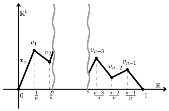
Figure 1. Function $x_v$.

Then $x_v\left(\frac{i}{n}\right)=v_i,$ for $i=0,\cdots ,n$ and we put

$$x\left[i\right]:=x_v\left(\frac{i}{n}\right)$$

(12)

and set

$$X_n:=\left\{x_v:v\in {\left({\mathbb{R}}^k\right)}^{n-1}\right\}.$$

Then $dim{X}_n=k(n-1)$ and of course $X_n\subset H_0^1(0,1;{\mathbb{R}}^k)$ is a closed subspace and $\overline{{\bigcup }_{n\in \mathbb{N}}{X}_n}=\mathcal{H}$. Moreover, for every $x\in X_n$ we calculate

$$\begin{array}{cc}\hfill {\int }_0^1{\left|\dot{x}\left(t\right)\right|}^{2}dt& =\sum _{i=1}^n{\int }_{\frac{i-1}{n}}^{\frac{i}{n}}{\left|\frac{d}{dt}\left(x[i-1]+n\left(t-\frac{i}{n}\right)(x\left[i\right]-x[i-1])\right)\right|}^{2}dt\hfill \\ \hfill & =\sum _{i=1}^n{\int }_{\frac{i-1}{n}}^{\frac{i}{n}}{n}^2{|x\left[i\right]-x[i-1]|}^2=n\sum _{i=1}^n{|\Delta x[i-1]|}^2.\hfill \end{array}$$

(13)

We use a standard approximation of an integral, namely

$${\int }_0^{1}F(t,x\left(t\right))dt\approx \sum _{i=0}^{n-1}F\left(\frac{i}{n},x\left(\frac{i}{n}\right)\right)\left(\frac{i+1}{n}-\frac{i}{n}\right)=\frac{1}{n}\sum _{i=1}^{n-1}F\left(\frac{i}{n},x\left[i\right]\right).$$

As it was mentioned in the Introduction, in order to obtain a family of discrete problems approximating the given problem (1), we firstly need to construct discretization of functional $\mathcal{E}$ that is a family of functionals ${\mathcal{E}}_n:H_0^1(0,1;{\mathbb{R}}^k)⟶\mathbb{R}$, $n\in \mathbb{N}$, defined by the formulas

$${\mathcal{E}}_n\left(x\right)=\frac{n}{2}\sum _{i=1}^n{|\Delta x[i-1]|}^2-\frac{1}{n}\sum _{i=1}^{n-1}F\left(\frac{i}{n},x\left[i\right]\right).$$

(14)

Functional ${\mathcal{E}}_n$ are well defined since $H_0^1(0,1;{\mathbb{R}}^k)\hookrightarrow C([0,1],{\mathbb{R}}^k)$ which means that every element of $H_0^1(0,1;{\mathbb{R}}^k)$ is continuous and thus it makes sense to calculate it at selected points. Moreover, we obtain

$$\begin{array}{cc}\hfill ⟨{\mathcal{E}}_n^{\prime }\left(x\right),y⟩& =\sum _{i=1}^n\Delta x[i-1]\Delta y[i-1]-\frac{1}{n}\sum _{i=1}^{n-1}f\left(\frac{i}{n},x\left[i\right]\right)y\left[i\right]\hfill \\ \hfill & =-n\sum _{i=1}^{n-1}{\Delta }^{2}x[i-1]y\left[i\right]-\frac{1}{n}\sum _{i=1}^{n-1}f\left(\frac{i}{n},x\left[i\right]\right)y\left[i\right].\hfill \end{array}$$

Therefore, recalling convention (12), every critical point of ${\mathcal{E}}_n$ solves (2).

Remark 6.

Observe that the values of ${\mathcal{E}}_n$, and hence the solvability of (1), depend only on values at $\frac{1}{n},\cdots ,\frac{n-1}{n}$. In the original Ritz method we minimize the following functional

$$X_n\ni x⟼\frac{n}{2}\sum _{i=1}^n{|\Delta x\left[i\right]|}^2-{\int }_0^{1}F(t,x\left(t\right))dt\in \mathbb{R}.$$

The second component cannot be equal $\frac{1}{n}{\sum }_{i=1}^{n-1}F\left(\frac{i}{n},x\left[i\right]\right)$ since in that case F should be piecewise constant, which means it is not continuous unless it is constant everywhere. This is why there is an apparent difference between Theorem 3 and examples in which algebraic discretization cannot be solved.

It is well known that the first eigenvalue for the second order differential operator with Dirichlet boundary conditions serves as the best constant in the Poincaré inequality, i.e.,

$${\pi }^2=\underset{x\in H_0^1(0,1;{\mathbb{R}}^k)}{inf}\frac{{\displaystyle {\int }_0^1{\left|\dot{x}\left(t\right)\right|}^{2}dt}}{{\displaystyle {\int }_0^1{\left|x\left(t\right)\right|}^{2}dt}}.$$

This explains why the constant in Assumption 3 is chosen so that $\gamma <{\pi }^2$.

For a given $n\in \mathbb{N}$, $n\ge 2$, we define

$$c_n:=\underset{x\in X_n\setminus \left\{0\right\}}{inf}\frac{{\displaystyle n\sum _{i=1}^n{|\Delta x[i-1]|}^2}}{{\displaystyle \frac{1}{n}\sum _{i=1}^{n-1}{\left|x\left[i\right]\right|}^2}}$$

(15)

and

$$D_n=n^2{\left[\begin{array}{ccccc}2& -1& 0& \cdots & 0\\ -1& 2& -1& \cdots & 0\\ ⋮& \ddots & \ddots & \ddots & ⋮\\ 0& \cdots & -1& 2& -1\\ 0& \cdots & 0& -1& 2\end{array}\right]}_{(n-1)\times (n-1)}.$$

(16)

Lemma 3.

For every $n\in \mathbb{N}$, $n\ge 2$, we have

$$c_n=2n^2\left(1-cos\left(\frac{\pi }{n}\right)\right).$$

Sequence ${\left(c_n\right)}_n$ is increasing, i.e., $c_2<c_3<\cdots <{\pi }^2$ and

$$\underset{n\to \infty }{lim}{c}_n={\pi }^2.$$

Proof. 

Assume that $k=1$. Take $x\in X_n$ and denote

$$u:={\left[\begin{array}{c}x\left[1\right]\\ ⋮\\ x[n-1]\end{array}\right]}_{(n-1)\times 1}.$$

Therefore, since $\sigma \left(D_n\right)= \left\{2n^2\left(1-cos\left(\frac{\pi }{n}\right)\right),\cdots ,2n^2\left(1-cos\left(\frac{(n-1)\pi }{n}\right)\right)\right\}$, see [2], we obtain that

$$\begin{array}{c}\hfill n^2\sum _{i=1}^n{|\Delta x[i-1]|}^2=n^2{u}^T{D}_{n}u\ge n^2\left(2-2cos\left(\frac{\pi }{n}\right)\right)u^{T}u=c_n\sum _{i=1}^{n-1}{\left|x\left[i\right]\right|}^2.\end{array}$$

Now, let $k\in \mathbb{N}$, $k\ge 2$. Then $x=(x_1,\cdots ,x_k)$, where $x_j:[0,1]⟶\mathbb{R}$. Hence, by what we have already proved, it follows

$$\begin{array}{cc}\hfill \sum _{i=1}^n{|\Delta x[i-1]|}^2& =\sum _{i=1}^n\sum _{j=1}^k|\Delta x_j{[i-1]|}^2=\sum _{j=1}^k\sum _{i=1}^n{|\Delta x_j[i-1]|}^2\hfill \\ \hfill & \ge n^2\left(2-2cos\left(\frac{\pi }{n}\right)\right)\sum _{j=1}^k\sum _{i=1}^n{\left|x_j[i-1]\right|}^2\hfill \\ \hfill & =n^2\left(2-2cos\left(\frac{\pi }{n}\right)\right)\sum _{i=1}^n{\left|x[i-1]\right|}^2.\hfill \end{array}$$

□

We have already proved that set of critical points of ${\mathcal{E}}_n^{\prime }$ and set of solutions to (2) coincide. Now we turn to showing that all but a finite number of discrete problems have solutions which are uniformly (with respect to n) bounded.

Proposition 1.

Let Assumptions 1–3 be satisfied. Then there exists $N\in \mathbb{N}$ such that for every $n\ge N$, problem (2) posses a unique solution on $X_n$. Moreover, there is a constant $M>0$ such that $∥x_n∥\le M$ for all $n\ge N$.

Proof. 

Due to Lemma 3 there exists $N\in \mathbb{N}$ such that $\gamma <c_n$ for all $n\ge N$. We restrict functional ${\mathcal{E}}_n$ to space $X_n$. Then operator ${\mathcal{E}}_n^{\prime }:X_n⟶{\left(X_n\right)}^{\ast }$ is $(c_n-\gamma )$-strongly monotone for every $n\ge N$. Applying Lemma 1 we get the solvability for $n\ge N$. Since $x_n$ solves (2), then by direct calculations and by definition of $c_n$, see (15), we obtain

$$\begin{array}{cc}\hfill \parallel x_n{\parallel }^2& =n\sum _{i=1}^n{|\Delta x_n[i-1]|}^2=-n\sum _{i=1}^{n-1}{\Delta }^2{x}_n[i-1]x_n\left[i\right]=\frac{1}{n}\sum _{i=1}^{n-1}f\left(\frac{i}{n},x_n\left[i\right]\right)x_n\left[i\right]\hfill \\ \hfill & =\frac{1}{n}\sum _{i=1}^{n-1}\left(f\left(\frac{i}{n},x_n\left[i\right]\right)-f\left(\frac{i}{n},0\right)\right)x_n\left[i\right]+\frac{1}{n}\sum _{i=1}^{n-1}f\left(\frac{i}{n},0\right)x_n\left[i\right]\hfill \\ \hfill & \le \frac{1}{n}\sum _{i=1}^{n-1}\gamma {\left|x_n\left[i\right]\right|}^2+{\left(\frac{1}{n}\sum _{i=1}^{n-1}{\left|f\left(\frac{i}{n},0\right)\right|}^2\right)}^{\frac{1}{2}}{\left(\frac{1}{n}\sum _{i=1}^{n-1}{\left|x_n\left[i\right]\right|}^2\right)}^{\frac{1}{2}}\hfill \\ \hfill & \le \frac{\gamma }{c_n}n\sum _{i=1}^n|\Delta x_n{[i-1]|}^2+\underset{0\le t\le 1}{sup}\left|f(t,0)\right|{\left(\frac{n}{c_n}\sum _{i=1}^n{|\Delta x_n[i-1]|}^2\right)}^{\frac{1}{2}}\hfill \\ \hfill & =\frac{\gamma }{c_n}\parallel x_n{\parallel }^2+\underset{0\le t\le 1}{sup}\left|f(t,0)\right|\parallel x_n\parallel \le \frac{\gamma }{c_N}\parallel x_n{\parallel }^2+\underset{0\le t\le 1}{sup}\left|f(t,0)\right|\parallel x_n\parallel \hfill \end{array}$$

Finally, for every $n\ge N$ we have

$$\parallel x_n\parallel \le \frac{{sup}_{0\le t\le 1}\left|f(t,0)\right|}{1-\frac{\gamma }{c_N}}.$$

The above formula makes sense since $t⟼f(t,0)$ is continuous on $[0,1]$. □

5. Convergence of Discretizations

In this section we consider the sequence of solutions to discretizations and its convergence. We must investigate its nature, i.e., prove that it is a minimizing sequence to functional $\mathcal{E}$ and next investigate its convergence. Let us recall, after [18],

Lemma 4.

Let $x\in H_0^1(0,1;{\mathbb{R}}^k)$. Then $|x\left(t\right)-x\left(s\right)|\le {\parallel x\parallel |t-s|}^{\frac{1}{2}}$ for all $t,s\in [0,1]$.

Proposition 2.

Let Assumptions 1 and 2 be satisfied. Then the sequence of functionals ${\left({\mathcal{E}}_n\right)}_n$ converges to $\mathcal{E}$ uniformly on $B_r\left(0\right)=\{x\in \mathcal{H}:\parallel x\parallel \le r\}$ for every $r>0$.

Proof. 

Due to the Sobolev inequality

$$\underset{0\le t\le 1}{sup}\left|x\left(t\right)\right|\le {\left({\int }_0^1{\left|\dot{x}\left(t\right)\right|}^{2}dt\right)}^{\frac{1}{2}}$$

we obtain that for every $x\in B_r\left(0\right)$ we have $\left|x\right(t\left)\right|\le r$ for every $t\in [0,1]$. Take $\epsilon >0$. Since F is uniformly continuous on $[0,1]\times B_r\left(0\right)$ and due to Lemma 4, one can find $N\in \mathbb{N}$ such that

$$\left|F(t,x\left(t\right))-F\left(\frac{i}{n},x\left[i\right]\right)\right| <\epsilon$$

for all $x\in B_r\left(0\right)$, $n>N$, $i=1\cdots n$ and $t\in \left[\frac{i}{n},\frac{i+1}{n}\right]$. Therefore, bearing in mind (13), we obtain that for every $x\in B_r\left(0\right)$ one has

$$\begin{array}{cc}\hfill |\mathcal{E}\left(x\right)-{\mathcal{E}}_n\left(x\right)|& = \left|{\int }_0^{1}F(t,x\left(t\right))dt-\frac{1}{n}\sum _{i=1}^{n-1}F\left(\frac{i}{n},x\left[i\right]\right)\right|\hfill \\ \hfill & \le \sum _{i=1}^{n-1}{\int }_{\frac{i-1}{n}}^{\frac{i}{n}}\left|F(t,x\left(t\right))-F\left(\frac{i}{n},x\left[i\right]\right)\right|\le \frac{1}{n}\sum _{i=1}^n\epsilon =\epsilon .\hfill \end{array}$$

Since $\epsilon$ was taken arbitrary, we have ${\mathcal{E}}_n{{|}_{B_r\left(0\right)}\rightrightarrows \mathcal{E}|}_{B_r\left(0\right)}$. □

Remark 7.

Recall that under Assumptions 1–3 functional $\mathcal{E}$ is coercive, see Lemma 1 and Theorem 4. Hence we can restrict considerations to some bounded set where the minimizer is located. Therefore, by Proposition 2,

$$\underset{n\to \infty }{lim}\underset{x\in X_n}{inf}{\mathcal{E}}_n\left(x\right)=\underset{n\to \infty }{lim}\underset{x\in X_n}{inf}\mathcal{E}\left(x\right).$$

Denoting by ${\left(x_n\right)}_n$, for enough large n, a sequence of solutions to (2), we see that it is bounded by Proposition 1 and moreover, it is a minimizing sequence for $\mathcal{E}$. Minimizing sequence to our action functional $\mathcal{E}$ converges strongly (i.e. in norm) to the minimizer. This is the content of the next theorem which strengthens the usual assertion which stems from the direct method implying that the minimizing sequence is weakly convergent. Thus we have also some improvement on results from [18], see Corollary 1.3.

Theorem 5.

Let Assumptions 1 and 2 be satified. If ${\left(x_n\right)}_n$ is a bounded minimizing sequence of $\mathcal{E}$, then (1) has a solution $x_{\ast }$ such that $x_n\to x_{\ast }$ up to subsequence. Therefore, if $x_{\ast }$ is a unique solution, then $x_n\to x_{\ast }$.

For the proof see [20]. As a consequence of Proposition 1 Theorems 4 and 5 we obtain

Theorem 6.

Let Assumptons 1–3 be satisfied. Then there exists $N\in \mathbb{N}$ such that (2) has a unique solution $x_n$ for every $n\ge N$. Moreover (1) has also a unique solution $x_{\ast }$ and $x_n\to x_{\ast }$.

Remark 8.

Let us recall that every convergence in Theorems 5 and 6 are understood in $H_0^1$-sense. In particular, since $H_0^1([0,1],{\mathbb{R}}^k)\hookrightarrow C(0,1],{\mathbb{R}}^k)$ is continuous, we obtain

$$\underset{0\le i\le n}{max}\left|x_n\left[i\right]-x_{\ast }\left(\frac{i}{n}\right)\right|\le \underset{0\le t\le 1}{sup}|x_n\left(t\right)-x_{\ast }\left(t\right)|\le \parallel x_n-x^{\ast }\parallel \to 0.$$

The nonlinear terms which are tackled by our assumptions are as follows.

Example 1.

The following functions $f_1,f_2,f_3:[0,1]\times \mathbb{R}⟶\mathbb{R}$ satisfy Assumptions 1–3.

• $f_1(t,x)=\frac{t-{\pi }^{2}sin\left(x\right)}{2x^2+4}$;
• $f_2(t,x)={\pi }^{2}x{e}^{\pi -t}+arctan\left(x\right)+e^t$;
• $f_3(t,x)=({\pi }^2-1)x-x^3+t^3-sin\left(t\right)$.

As long as Theorem PropositionConvergenceOfDiscretizations provides convergence of solutions to discretizations ${\left(x_n\right)}_n$ to the solution to continuous problem $x_{\ast }$, it gives no information about the rate of convergence $x_n\to x_{\ast }$. It turns out that in such investigation the constant $\gamma$ appearing in Assumption 3 may be crucial as well as its relation to the first eigenvalue of a Dirichlet problem.

Some Numerical Phenomena (Whole Subsection Has Been Changed)

We start an example of nonlinearity where both, continuous solution and solution to the associated discretizations coincide.

Example 2.

Consider a nonlinearity $f(t,x)=\alpha x$, $\alpha <{\pi }^2$. Then both, (1) and (2), have a trivial solution $x\equiv 0$.

It is worth mentioning that nonlinearity considered in the Example 2 is associated with a classical eigenvalue problem of the form

$$\left\{\begin{array}{c}-\ddot{x}=\alpha x,\hfill \\ x\left(0\right)=x\left(1\right)=0.\hfill \end{array}\right.$$

Assumption $\alpha <{\pi }^2$ can be reformulated in the following manner: a constant $\alpha$ is less then the first eigenvalue of the second order Laplace operator with Dirichlet boundary value conditions. For more details on the eigenvalue we refer to [18]. It occurs that an interesting phenomena can be observed by considering a family of nonhomogeneous eigenvalue problems of the form

$$\left\{\begin{array}{c}-\ddot{x}=\alpha x+{\pi }^{2}sin\left(\pi t\right)-\alpha sin\left(\pi t\right),\hfill \\ x\left(0\right)=x\left(1\right)=0.\hfill \end{array}\right.$$

(17)

where $\alpha \in \mathbb{R}$. Together with (17) we consider their discretizations of the form

$$\left\{\begin{array}{c}-n^2{\Delta }^{2}x[i-1]=\alpha x\left[i\right]+{\pi }^{2}sin\left(\frac{\pi i}{n}\right)-\alpha sin\left(\frac{\pi i}{n}\right),\hfill \\ x\left[0\right]=x\left[n\right]=0,\hfill \end{array}\right.$$

(18)

where $n\in \mathbb{N}$ derived according to the scheme which we have introduced in this paper. Note that $t⟼sin\left(\pi t\right)$ is a solution to (17) for every $\alpha$. Moreover, due to Theorem 4, this function is a unique solution to (17) provided $\alpha <{\pi }^2$. Using Theorem 6 and Lemma 3 we see that (18) has a unique solution $x_{n,\alpha }$ for all $\alpha <{\pi }^2$ if n is such that $\alpha <2n^2\left(1-cos\left(\frac{\pi }{n}\right)\right)$. For such a pairs $(n,\alpha )$ we put

$${ϵ}_{n,\alpha }:={\left(\sum _{i=1}^{n-1}{\left|sin\left(\frac{\pi i}{n}\right)-x_{n,\alpha }\left[i\right]\right|}^2\right)}^{\frac{1}{2}},$$

(19)

which is a an error correction between continuous and discrete solution. Due to Theorem 6 we see that

$$\underset{n\to \infty }{lim}\frac{{ϵ}_{n,\alpha }}{\sqrt{n}}=0$$

for every $\alpha <{\pi }^2$. We put also

$${ϵ}_{n,\alpha }^d:=\sum _{i=1}^{n-1}\left|n^2{\Delta }^{2}x[i-1]+f_{k,\alpha }\left(\frac{i}{n},x\left[i\right]\right)\right|,$$

where $x\in X_n$, $\alpha <{\pi }^2$. This expression describes the error between x and $x_{n,\alpha }$. For visualisations of the error correction we use the logarithmic scale, namely we plot $ln\left(1+{10}^6·\right.$$\left.{ϵ}_{n,\alpha }\right)$. Error of discretization ${ϵ}_{n,\alpha }^d$ is held on ${10}^{-6}$ level. To study the rate of convergence of ${\left({ϵ}_{n,\alpha }\right)}_n$ we use numerical experiments.

We see that the accuracy of discretization can strongly depend on the strong monotonicity constant $\gamma ={\pi }^2-\alpha$, see Figure 2. One can demonstrate that function $f_{\alpha }$ satisfy Assumption 3 iff $\alpha <{\pi }^2$. Moreover, the associated energy functionals are not convex if $\alpha >{\pi }^2$. Hence ${\pi }^2$ is, in this sense, a critical constant for $f_{\alpha }$. It is very important that the observed phenomena is not a general rule, which can be suggested by Example 2.

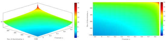
Figure 2. Plot of $ln\left(1+{10}^6·{ϵ}_{n,\alpha }\right)$ depending on $\alpha$ and n.

Example 3.

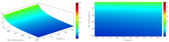
We consider nonlinearities of the form

$$\begin{array}{cc}\hfill f_{1,\alpha }& =\alpha x-e^x+{\pi }^{2}sin\left(\pi t\right)-\alpha sin\left(\pi t\right)+e^{sin\left(\pi t\right)},\hfill \\ \hfill f_{2,\alpha }& =\alpha sin\left(x\right)+{\pi }^{2}sin\left(\pi t\right)-\alpha sin(sin\left(\pi t\right)),\hfill \end{array}$$

where $\alpha \in (-{\pi }^2{\pi }^2)$. Note that $t⟼sin\left(\pi t\right)$ is, as before, the solution to the continuous problems (1) for $f=f_{1,\alpha }$ and $f=f_{2,\alpha }$. Denote by $x_{k,n,\alpha }$, for n satisfying $\alpha <2n^2\left(1-cos\left(\frac{\pi }{n}\right)\right)$, a unique solution to

$$\left\{\begin{array}{c}-n^2{\Delta }^{2}x[i-1]=f_{k,\alpha }\left(\frac{i}{n},x\left[i\right]\right),\hfill \\ x\left[0\right]=x\left[n\right]=0,\hfill \end{array}\right.$$

(20)

for $k=1,2$. The existence of such $x_{k_n}$ follows from Proposition 6 and Lemma 3. We consider an error correction between continuous and discrete solution given by the formula analogous to (19), namely

$${ϵ}_{k,n,\alpha }:={\left(\sum _{i=1}^{n-1}{\left|sin\left(\frac{\pi i}{n}\right)-x_{k,n,\alpha }\left[i\right]\right|}^2\right)}^{\frac{1}{2}}.$$

Figure 3 and Figure 4 depict an error corrections for nonlinearities $f_{1,\alpha }$ and $f_{2,\alpha }$, respectively.

Figure 3. Plot of $ln\left(1+{10}^6·{ϵ}_{1,n,\alpha }\right)$ depending on $\alpha$ and n.

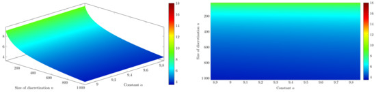
Figure 4. Plot of $ln\left(1+{10}^6·{ϵ}_{2,n,\alpha }\right)$ depending on $\alpha$ and n.

The quantity ${ϵ}_{k,n\alpha }$, for $k=1,2$, strongly depends on the size of disretization. However we observe no significant correlation with a constant α.

6. Conclusions

From the formal content of the paper the following observations can be underlined (however informal in their nature):

• Usage of a Sobolev space setting for our problem allows us to consider a continuous and discrete problems as an elements in the same spaces. Therefore we can use a general and easy tools from functional analysis (Ritz and Direct Method of Variational Method together with some monotonicity relations).
• Algebraic discretizations are of use since, for sufficiently large n, the solvability of a continuous problem provides a solvability of a discrete one (at in least if we use the mentioned Direct Method).
• There may be significant differences with handling homogeneous (Example 2) and nonhomogeneous first eigenvalue problem and its discretizations.
• The above mentioned phenomena is not a general rule. It strongly depends on the precise form of the nonlinearity.

References

- Gaines, R. Difference equations associated with boundary value problems for second order nonlinear ordinary differential equations. SIAM J. Numer. Anal. 1974, 11, 411–434. [Google Scholar] [CrossRef]
- Kelley, W.G.; Peterson, A.C. Difference Equations: An Introduction with Applications, 2nd ed.; Harcourt/Academic Press: San Diego, CA, USA, 2001. [Google Scholar]
- Anderson, D.R.; Tisdell, C.C. Discrete approaches to continuous boundary value problems: Existence and convergence of solutions. Abstr. Appl. Anal. 2016, 2016, 3910972. [Google Scholar] [CrossRef]
- Thompson, H.B.; Tisdell, C.C. The nonexistence of spurious solutions to discrete, two-point boundary value problems. Appl. Math. Lett. 2003, 16, 79–84. [Google Scholar] [CrossRef]
- Rachůnková, I.; Tisdell, C.C. Existence of non-spurious solutions to discrete Dirichlet problems with lower and upper solutions. Nonlinear Anal. 2007, 67, 1236–1245. [Google Scholar] [CrossRef]
- Rachůnková, I.; Tisdell, C.C. Existence of non-spurious solutions to discrete boundary value problems. Aust. J. Math. Anal. Appl. 2006, 3, 6. [Google Scholar]
- Bełdziński, M.; Galewski, M. Global diffeomorphism theorem applied to the solvability of discrete and continuous boundary value problems. J. Diff. Equat. Appl. 2018, 24, 277–290. [Google Scholar] [CrossRef]
- Galewski, M.; Schmeidel, E. Non-spurious solutions to discrete boundary value problems through variational methods. J. Differ. Equ. Appl. 2015, 21, 1234–1243. [Google Scholar] [CrossRef][Green Version]
- Chen, Y.; Zhou, Z. Existence of Three Solutions for a Nonlinear Discrete Boundary Value Problem with ϕc-Laplacian. Symmetry 2020, 12, 1839. [Google Scholar] [CrossRef]
- Lin, L.; Liu, Y.; Zhao, D. Multiple Solutions for a Class of Nonlinear Fourth-Order Boundary Value Problems. Symmetry 2020, 12, 1989. [Google Scholar] [CrossRef]
- Agarwal, R.P. Difference Equations and Inequalities: Theory, Methods, and Applications; Marcel Dekker: New York, NY, USA, 1992. [Google Scholar]
- Elaydi, S. An Introduction to Difference Equations; Springer Science & Business Media: Heidelberg, Germany, 2005. [Google Scholar]
- Banasiak, J. Mathematical Modelling in One Dimension. An Introduction via Difference and Differential Equations; African Institute of Mathematics (AIMS) Library Series; Cambridge University Press: Cambridge, UK, 2013. [Google Scholar]
- Kaplan, D.; Glass, L. Understanding Nonlinear Dynamics; Corrected Reprint of the 1995 Original; Textbooks in Mathematical Sciences; Springer: New York, NY, USA, 1998. [Google Scholar]
- Drábek, P.; Milota, J. Methods of Nonlinear Analysis. Applications to Differential Equations, 2nd ed.; Birkhäuser Advanced Texts Basler Lehrbücher; Springer: Basel, Switzerland, 2013. [Google Scholar]
- Fučík, S.; Kufner, A. Nonlinear Differential Equations. Studies in Applied Mechanics. 2; Elsevier Scientific Publishing Company: Amsterdam, The Netherlands; Oxford, UK; New York, NY, USA, 1980; 359p. [Google Scholar]
- Agarwal, R.P. On multipoint boundary value problems for discrete equations. J. Math. Anal. Appl. 1983, 96, 520–534. [Google Scholar] [CrossRef]
- Mawhin, J. Problèmes de Dirichlet Variationnels Non Linéaires; Les Presses de l’Universit é de Montréal: Montreal, QC, Canada, 1987. [Google Scholar]
- Gajewski, H.; Gröger, K.; Zacharias, K. Nichtlineare Operatorgleichungen und Operatordifferentialgleichungen; Akademie–Verlag: Berlin, Germany, 1974. [Google Scholar]
- Galewski, M. On variational nonlinear equations with monotone operators. Adv. Nonlinear Anal. 2021, 10, 289–300. [Google Scholar] [CrossRef]
Publisher’s Note: MDPI stays neutral with regard to jurisdictional claims in published maps and institutional affiliations. |
© 2021 by the authors. Licensee MDPI, Basel, Switzerland. This article is an open access article distributed under the terms and conditions of the Creative Commons Attribution (CC BY) license (http://creativecommons.org/licenses/by/4.0/).