Abstract
This study discusses model development for response variables following a bivariate gamma distribution using three-parameters, namely shape, scale and location parameters, paying attention to spatial effects so as to produce different parameter estimator values for each location. This model is called geographically weighted bivariate gamma regression (GWBGR). The method used for parameter estimation is maximum-likelihood estimation (MLE) with the Berndt–Hall–Hall-Hausman (BHHH) algorithm approach. Parameter testing consisted of a simultaneous test using the maximum-likelihood ratio test (MLRT) and a partial test using Wald test. The results of GWBGR modeling three-parameters with fixed weight bisquare kernel showed that the variables that significantly affect the rate of infant mortality (RIM) and rate of maternal mortality (RMM) are the percentage of poor people, the percentage of obstetric complications treated, the percentage of pregnant mothers who received Fe3 and the percentage of first-time pregnant mothers under seventeen years of age. While the percentage of households with clean and healthy lifestyle only significant in several regencies and cities.
1. Introduction
Distribution is a statistical concept used in data research. Statisticians seeking to identify the outcomes and probabilities of a particular study will chart measurable data points from a data set, resulting in a probability distribution diagram. Statisticians can identify the development of either a discrete or continuous distribution by the nature of the outcomes to be measured. Discrete distributions have a countable number of outcomes, which means that the potential outcomes can be put into a list. A continuous distribution is built from outcomes that fall in a continuum.
One type of continuous distribution is gamma distribution. There is some research on gamma distribution that focuses on the estimation of parameters, such as parameter estimation of gamma distribution with three-parameters using maximum marginalized order statistics likelihood estimation (MMosLE). Then the results obtained were compared with the second alternative method is the method of location and scale parameters free maximum-likelihood estimators (LSPF-MLE) and Bayesian methods (BL) [1]. Then the gamma distribution parameters for k-variate of three-parameters were estimated using the heuristic approach. The estimation results were obtained through simulation using the maximum likelihood function, the maximum product of spacing (MPS) and the least square (LS), where LS produces a better estimate value [2]. Rahayu, Purhadi, Sutikno and Prastyo [3] conducted a study on the theory of parameter estimation and hypothesis testing for trivariate gamma regression. As a development, Rahayu, Purhadi, Sutikno and Prastyo [4] studied the theory of parameter estimation, hypothesis testing and its application to multivariate gamma regression.
Gamma regression is used for modeling cases with continuous response variables that have a positive skewness. Gamma regression for two response variables is called bivariate gamma regression (BGR). This research focuses on parameter estimation using the MLE method and simultaneous hypothesis testing using MLRT and partially using the Wald test.
Each regression model produces parameters that apply globally to all locations’ analyzed observations. The interpretation of the global model assumes that each observation locations have the same characteristics. However, in fact, there are certain cases that each location has different characteristics. Differences in these characteristics are influenced by geographical factors, economic, cultural or other factors so that the presence of spatial effects needs to be considered. Regression models that take into account the spatial heterogeneity that is geographically weighted regression (GWR). GWR is part of spatial analysis with weighting based on the position or the distance of the location of the observations with other observation sites [5].
Research on the GWR had been done and applied in many cases in fields, such as health, the environment and household items, for such modeling cases as the proportion of households that have a telephone in the state of Sao Paulo, Brazil [6]. A study analyzing the causes of haze pollution in China, the results showed that the GWR model performed better than global models [7]. And a study investigating the relationship between the level of disease with social and economic characteristics in Tokyo [8].
The GWR model for data with a two-parameter gamma distribution has been carried out both on univariate and bivariate data. Research on parameter estimation and hypothesis testing models gamma geographically weighted regression (GWGR). Researchers using the maximum-likelihood estimation method to find parameter estimation, but the results show that the MLE parameter estimation with no closed-form, then the numerical optimization using algorithm Broyden–Fletcher–Goldfarb–Shanno (BFGS) [9]. Then in bivariate data, that is modeling the case of the rate of maternal mortality (RMM) and rate of infant mortality (RIM) in North Sumatra province in 2017 with geographically weighted bivariate gamma regression (GWBGR).
RIM and RMM are examples of quantitative data. This issue was even included in the Sustainable Development Goals (SDGs), which were declared by the member states of the United Nations (UN) as a goal toward global development as a follow-up program of the Millennium Development Goals (MDGs). SDGs targets for maternal and child health, namely the achievement of RMM, are less than 70 per 100,000 live births (KH), and RIM as low as 25 per 1000 KH [10]. The MDG target for RMM is 102/100,000 KH, but the RMM in North Sulawesi, Gorontalo and Central Sulawesi, respectively, for 169, 253.42 and 208 [11,12,13], means that the target is not reached. RIM has met the MDG target which is below 32/1000 KH, but from year to year RIM has not experienced a significant decline for the three provinces.
Here is shown a histogram of the data RIM and RMM for two-parameter gamma and gamma three-parameters.
Figure 1 and Figure 2 show that the shape of the histogram of data RIM and RMM have a pattern similar to the gamma three-parameters compared with the two parameters; this is due to the role of the location parameter gamma distribution of three-parameters, namely, shifting the distribution in the horizontal axis.
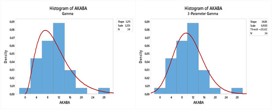
Figure 1.
Rate of infant mortality (RIM) histogram with gamma distribution of two parameters and three-parameters.
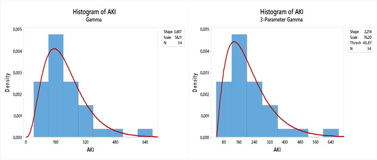
Figure 2.
Rate of maternal mortality (RMM) histogram with gamma distribution of two parameters and three-parameters.
Currently, research related to gamma regression is limited to the number of response variables and does not involve spatial effects. Therefore, in this study, we developed a regression involving two response variables that followed a bivariate gamma distribution and involved spatial effects.
Previous studies that discuss GWGR and GWBGR are limited to two parameters: the shape and scale parameters. As shown in Figure 1 and Figure 2, the RIM and RMM data from the province of North Sulawesi, Gorontalo and Central Sulawesi, this research models RIM and RMM with three-parameters where the two are correlated and gamma distribution. The focus of this study is to determine the parameter estimator and test statistics BGR and GWBGR for three-parameters in the case of RIM and RMM in North Sulawesi, Gorontalo and Central Sulawesi. If the MLE method produces an equation that is not closed form, BHHH methods will be used.
2. The Gamma Distribution
Y is a random variable with a gamma distribution for three-parameters that have a density function as follows [14].
When two gamma response variables distributed three-parameters that are not independent, it is called bivariate three-parameter gamma distribution. Suppose a random variable that is independent with , i = 1, 2. The density function for can be written as follows [14,15].
with and 0 for the other.
Here is a bivariate regression model two-parameter gamma.
with ,
PDF form gamma bivariate regression model is as follows [16].
with
The BGR model is shown in Equation (4) with a set of parameters ,
with
From Equation (4) is obtained and , Then and are substituted into Equation (1). The probability density function (PDF) for bivariate gamma distribution with three-parameters is:
The hypothesis for testing the correlation between the independent variables are:
Hypothesis 1 (H1).
(There was no relationship between Y1 and Y2).
Hypothesis 2 (H2).
(There is a relationship between Y1 and Y2).
The statistical test is:
The conclusion is to reject the null hypothesis if
Multicollinearity refers to a situation in which two or more independent variables in a multiple regression model are highly linearly related. The variance inflation factor (VIF) is often used to measure the degree of multicollinearity with the following formula [17].
with is the proportion of the variability between the other predictor variables.
Their effect on the spatial data can be seen from the spatial heterogeneity among locations. Spatial heterogeneity due to differences in the characteristics of the location of the observations with observations in other locations. Spatial heterogeneity testing can be performed using the hypothesis as follows.
Hypothesis 3 (H3).
Hypothesis 4 (H4).
there is at least one.
A statistical test is used:
with a variance-covariance matrix where the population below , a variance-covariance matrix under the null hypothesis.
Criteria for rejecting the null hypothesis if where k is the number of predictor variables with a significance level .
The formation of the Euclidean distance weighting function can be determined by using a kernel function as for some kernel functions proposed in [18].
- Fixed function Gaussian kernelwith:= the weighting of observations on the i-th location and the location of allg = bandwidth,= Euclidian distance.
- Adaptive kernel bisquare
- Fixed bisquare kernel
- Adaptive Gaussian kernel
The corrected Akaike information criterion (AICc) value is calculated by the following formula [19].
with n is the sample size and K is the number of parameters.
3. Data and Method
The data used from this study came from the publication of the Health Profile of North Sulawesi, Gorontalo and Central Sulawesi in 2016 and Welfare Statistics Publications North Sulawesi, Central Sulawesi and Gorontalo (Sulutenggo) in 2016. The observation unit was 34 regencies and cities in North Sulawesi, Gorontalo and Central Sulawesi. The data used were two response variables, i.e., rate of infant mortality and maternal mortality, with six predictor variables: the percentage of poor people, percentage of obstetric complications are handled, the percentage of pregnant mothers who received Fe3, the percentage of first-time pregnant mothers under seventeen years of age, the percentage of use of health facilities, and the percentage of households with clean and healthy lifestyle.
The parameter estimators are obtained using the MLE. The simultaneous test for GWBGR’s significance was done using MLRT. The partial test for individual parameter significance in GWBGR was done using the Wald test.
4. Discussion and Analysis
4.1. Parameter Estimation of GWBGR with Three-Parameters
Model GWBGR three-parameters can be formed as follows.
with GWBGR the model parameter estimation using maximum-likelihood estimation (MLE). The first step is to establish a likelihood function with the set parameters
The log-likelihood function is shown as follows.
The following is the log-likelihood function for each location.
The first derivative of the log-likelihood function for is:
The first derivative of the log-likelihood function for is:
The first derivative of the log-likelihood function for is:
The first derivative of the log-likelihood function for is:
The first derivative of the log-likelihood function for is:
The results showed that the derivative of the equation is shown in the form of implicit, so it is necessary to use numerical optimization is BHHH. BHHH procedure similar to that shown in the global model parameter estimation in which the iteration process stops when . BHHH iteration equation is as follows.
where
4.2. The Hypothesis Testing for GWBGR Model
4.2.1. The Similarity Model Test
Once the parameters were obtained good estimates for global and local models, the next step was testing the model in common use comparative value deviance global models and local models with a degree of freedom for the global model. The hypothesis is as follows.
Hypothesis 5 (H5).
Hypothesis 6 (H6).
at least one.
The criteria that reject the null hypothesis if where the degrees of freedom df1 and df2 global model is a local model-free interval and with a certain significance level (α). The deviance for GWBGR models can be obtained by looking and can be obtained by maximizing the likelihood function under the null hypothesis. The parameters were set under the null hypothesis . The log-likelihood function under the null hypothesis can be defined as follows.
Parameter estimator on the location of under the null hypothesis could be obtained by using MLE.
The first derivative of the log-likelihood function for is:
with .
The first derivative of the log-likelihood function for is:
The first derivative of the log-likelihood function for is:
The first derivative of the log-likelihood function for is:
The first derivative of the log-likelihood function for is:
The results of the first derivative of the log-likelihood function for each parameter are not closed form, so a numerical method is needed to obtain an estimator value for each parameter. Having obtained the results of parameter estimation, the next step is to define
4.2.2. The Simultaneous Test
A simultaneous test was used to determine the significance of the regression coefficients with the test statistics used is G2. The hypothesis used for simultaneous testing is as follows.
Hypothesis 7 (H7).
.
Hypothesis 8 (H8).
at least one.
The test statistic used is:
Reject the null hypothesis if G2 > with significance level α and v is the difference
4.2.3. The Partial Test
If the test was simultaneously or synchronously significant, then we proceeded with the partial test to determine which variables influenced the model. The hypothesis used in this test is:
Hypothesis 9 (H9).
Hypothesis 10 (H10).
The test statistic used is:
with , is a diagonal element corresponding to Reject the null hypothesis is
4.3. Descriptive Statistics and Testing Assumptions
The following are descriptive statistics for response and predictor variables for 34 regencies and cities in North Sulawesi, Gorontalo and Central Sulawesi.
Table 1 shows that the average RIM and RMM in 2016 were 10.463 and 209.6. The lowest percentage of poor people was located in the city of Manado, namely 5.24% and the highest percentage was located in Gorontalo at 78.35%. The average percentage of obstetric complications in the three provinces, which amounted to 15.95%. The average provision of Fe3 in pregnant mothers was 76.55%. The percentage of first-time pregnant mothers under seventeen years of age most likely in Central Sulawesi Parigi Moutong regency and the smallest in the city of Manado. The average use of health facilities in three provinces is 65.52%. The regencies has the lowest percentage for clean and healthy life behavior is Talaud regency, namely 27.12%.

Table 1.
Descriptive statistics for response and predictor variables.
Tests using the Kolmogorov–Smirnov show that the statistical value of each of Y1 and Y2 is 0.0985 (p-value: 0.864) and 0.0701 (p-value: 0.9919) in which p-value that is greater than the significance level of 5%, it can be concluded that the Y1 and Y2 follow the 3 parameter gamma distribution.
Before doing modeling necessary to examine the correlation between the response variables for the modeling requirements for the response variables of more than one is a correlation between these variables. T value = 3.2213, compared with ttable, |t| = 3.2213 > t table (0.025; 32) = 2.0369, then the conclusion is to reject the null hypothesis means that there is a relationship between the response variables Y1 and Y2.
Another requirement before modeling RIM and RMM is that there is no multicollinearity case between predictor variables. If the VIF value is greater than 10 indicates a case of multicollinearity. Table 2 shows that all the VIF value is smaller than 2 so that it can be concluded that there were no cases of multicollinearity.
Table 2.
Multicollinearity test.
4.4. Modeling RIM and RMM with BGR Three-Parameters
Modeling the RIM and RMM by BGR was carried out to obtain the factors that affect RIM and RMM in the province of North Sulawesi, Gorontalo and Central Sulawesi. The BGR model parameter estimation results are shown in Table 3 and Table 4. Then, perform the parameter hypothesis testing simultaneously using test statistic G2. Simultaneous test statistic values obtained 11,165.08 because the value is greater than 3.94, then the null hypothesis is rejected it means at least one independent variable that significantly influences the response variables. Then followed by a partial test pass. The value of the test statistic Z is shown in Table 3 and Table 4. With a significance level of 5% of the obtained, all predictor variables significantly influence the RIM and RMM for a value greater than .
Table 3.
RIM with bivariate gamma regression (BGR) parameter estimation model.
Table 4.
RMM with BGR parameter estimation model.
Based on Table 3 and Table 4, it can set up a global model for RIM and RMM in the province of North Sulawesi, Gorontalo and Central Sulawesi, respectively as follows.
Before modeling with GWBGR, three-parameters are required to test the spatial heterogeneity. The diperpoleh statistical value and the value of G is 129.3388 is 5.226. Clear that then the test is rejected the null hypothesis means RIM and RMM in North Sulawesi, Gorontalo and Central Sulawesi provinces has a spatial diversity between the regions.
4.5. Modeling the RIM and RMM with GWBGR Three-Parameters Models
Modeling the RIM and RMM by using the model GWBGR preceded by determining the geographic location of each regency and city in the province of North Sulawesi, Gorontalo, and Central Sulawesi then determine the optimum bandwidth value using the GCV. The next step is to obtain a weighting matrix, where it is necessary to first calculate the Euclidean distance. The selected weighting function that is weighted with a fixed-function bisquare kernel with the optimum bandwidth value is 33.265.
To test whether the geographical significance of the models will be tested using a model of statistical similarity with the F test following hypotheses.
Hypothesis 11 (H11).
Hypothesis 12 (H12).
at least one.
When the deviance for the global models is 11,165.08 and the deviance for the GWBGR models is 213,372.4, then the value of the F is 1.7791. Because the value of the F is greater than , the decision obtained is to reject the null hypothesis with a significance level of 5%. Hence, it is concluded that there are significant differences between the model parameters and GWBGR BGR three-parameters. Hypothesis test simultaneously on a parameter to determine whether the predictor variables affect RIM and RMM simultaneously. G2 test statistic obtained by 213,372.4116 where the value is greater than then the decision is to reject the null hypothesis, which is to say, simultaneously predictor variables affect the response variables with a significance level of 5%. It is next necessary partial testing to determine any predictor variables that affect the response variables.
Table 5 and Table 6 show parameter estimation results of the test statistic Z along RIM and RMM GWBGR model with three-parameters in one location Bolaang Mondow.
Table 5.
Values of RIM and geographically weighted bivariate gamma regression (GWBGR) parameter estimation models in the Bolaang Mongondow Regency.
Table 6.
Values of RMM and GWBGR parameter estimation models in the Bolaang Mongondow Regency.
The above results indicate that each predictor variable significant effect on RIM and RMM. This is evident from the value greater than the value Ztable with a significance level of 5% so that the GWBGR model for three-parameters as follows.
Based on the above models, it can be interpreted that an increase of one unit of the percentage of the poor population will increase RIM by exp (0.0022) = 1.0002 times and RMM by exp (0.0190) = 1.019 times, assuming other predictor variables are constant. Each increase of 1 unit of the percentage of use of health facilities will reduce RIM and RMM by exp (−0.0094) = 0.991 times and exp (−0.0051) = 0.995 times, assuming other predictor variables are constant. Each increase of one unit of the obstetric complications treated with assuming other predictor variables are constant, will increases RIM by exp (0.0046) = 1.0046 times and the RMM is 1.0076 times.
There is an increase of one percent of pregnant mothers under seventeen years, it will increase RIM, but the estimation results shows a different sign, namely a decrease RIM by exp (−0.1095) = 0.896 times and RMM by exp (−0.0264) = 0.974 times. This marks the difference allegedly caused by maternal age who have high-risk pregnancies, and maternal mortality-dominant causes occur in women aged over 35 years, compared to women aged under seventeen years. Each increase in households with clean and healthy lifestyle by one percent would reduce RIM in the Bolaang Mongondow Regency by exp (−0.0004) = 0.991 times, but increase RMM by exp (−0.0010) = 0.999 times, assuming other variables remain constant.
4.6. Selection of Best Model
The AICC value is a test statistic that can be used to determine which the best model among global models and local models in the modeling of RIM and RMM in the province of North Sulawesi, Gorontalo and Central Sulawesi.
The criterion for selecting the best model includes taking the model with the lowest AICC value. Table 7 shows that the model GWBGR with a bisquare fixed kernel function is the best model to model RIM and RMM in the province of North Sulawesi, Gorontalo and Central Sulawesi in 2016.
Table 7.
Comparison of AICC.
Figure 3 shows that there are two groups of regions based on common variables that significantly influence the mortality rate. The percentage of poor people, the percentage of obstetric complications treated, the percentage of pregnant mothers who received Fe3, the percentage of first-time pregnant mothers under seventeen years of age and the percentage of use of health facilities significantly affecting RIM in all regencies and cities in North Sulawesi, Gorontalo and Central Sulawesi provinces. In contrast, the percentage of households with clean and healthy lifestyle affects RIM in almost all regencies and cities in North Sulawesi, Gorontalo and Central Sulawesi provinces except North Mongondow Bolaang and Bone Bolango.
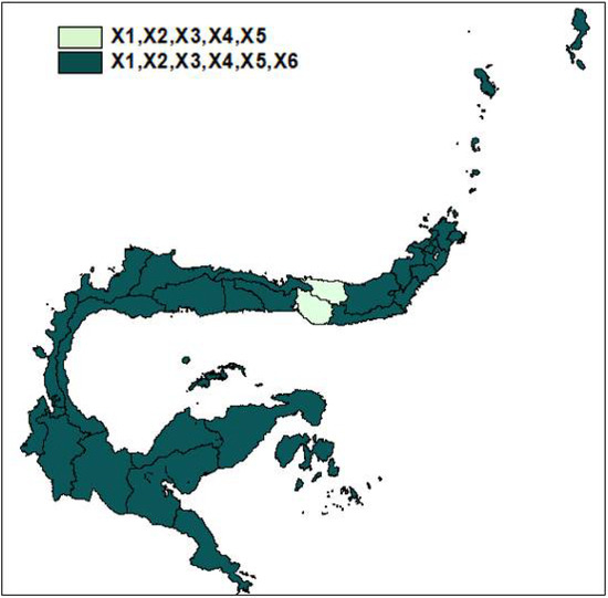
Figure 3.
Map of grouping variables significant impact of RIM.
Figure 4 shows that, based on common variables that significantly affect maternal mortality, there are two groups of regencies and cities in North Sulawesi, Gorontalo and Central Sulawesi provinces. Variables that are expected to affect RMM include the percentage of poor people, the percentage of obstetric complications treated, the percentage of pregnant mothers who received Fe3, the percentage of first-time pregnant mothers under seventeen years of age, the percentage of use of health facilities, and the percentage of households with clean and healthy lifestyle. In contrast, only the percentage of households with clean and healthy lifestyle significantly affect maternal mortality in 17 regencies and cities.
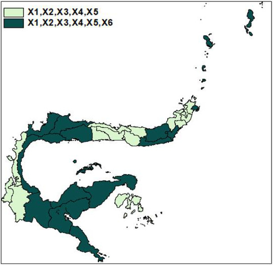
Figure 4.
Map of grouping variables significant impact of RMM.
In 1987, concerns regarding the impact of high RMM cases prompted WHO and other international organizations to establish “The safe motherhood initiative”, which has six main pillars, namely: family planning, antenatal care, maternity care, postnatal care, post-abortion care and sexually transmitted infection control, HIV and AIDS.
5. Conclusions
The parameter estimation of BGR and GWBGR models with three-parameters using MLE produces an equation that is not closed form, so it requires a numerical method to get an estimator value for each parameter. In this study, the numerical method used is BHHH. BGR and GWBGR modeling is applied to cases of RIM and RMM in the province of North Sulawesi, Gorontalo and Central Sulawesi. From the modeling results, RIM and RMM are influenced by the percentage of poor people, the percentage of obstetric complications treated, the percentage of pregnant mothers who received Fe3, the percentage of first-time pregnant mothers under seventeen years of age, the percentage of use of health facilities, and the percentage of households with clean and healthy lifestyle. The GWBGR modeling with fixed weight bisquare kernel produces two groups of regencies and cities based on the variables that significantly affect the RIM and two groups based on variables that significantly affect the RMM. The significant variables affecting RIM and RMM are the percentage of poor people, the percentage of obstetric complications treated, the percentage of pregnant mothers who received Fe3, the percentage of first-time pregnant mothers under seventeen years of age and the percentage of use of health facilities. The percentage of households with clean and healthy lifestyle does not significantly affect the RIM in the Bolaang Mongondow and Bone Bolango and does not significantly affect the RMM in the 17 regencies and cities. From these results, it is suggested for consideration at the next study that researchers use the mixed GWBGR model, get the data for response and predictor variables from the same source, and researchers can compare other test statistics for detecting multicollinearity.
Author Contributions
Conceptualization, G.H.W. and P.; methodology, G.H.W. and P.; software, G.H.W.; validation, G.H.W. and P.; formal analysis, G.H.W. and A.R.; investigation, G.H.W.; data curation, G.H.W. and P.; writing—original draft preparation, G.H.W. and A.R.; writing—review and editing, P. and A.R.; visualization, G.H.W. and A.R.; supervision, P.; project administration, P.; All authors have read and agreed to the published version of the manuscript.
Funding
This research is funded by the Deputy for Research and Development Strengthening, The Ministry of Research and Technology/The National Research and Innovation Agency with grant number: 3/E1/KP.PTNBH/2020.
Data Availability Statement
The data used from this study came from the publication of the Health Profile of North Sulawesi, Gorontalo and Central Sulawesi in 2016 and Welfare Statistics Publications North Sulawesi, Central Sulawesi and Gorontalo (Sulutenggo) in 2016. The links to find that data are:
Acknowledgments
The authors thank the editor and the reviewers for their constructive and helpful comments.
Conflicts of Interest
The authors declare no conflict of interest.
References
- Ouedraogo, E.A.J.; Some, B.; Gbete, S.D. On the Maximum Likelihood Estimation for the Three Parameter Gamma Distribution Based on Left Censored Samples. Sci. J. Appl. Math. Stat. 2017, 5, 147–163. [Google Scholar] [CrossRef]
- Vaidyanathan, V.S.; Lakshmi, R.V. Parameter Estimation in Multivariate Gamma Distribution. Stat. Optim. Inf. Comput. 2015, 3, 147–159. [Google Scholar] [CrossRef]
- Rahayu, A.; Purhadi; Sutikno; Prastyo, D.D. Trivariate Gamma Regression. IOP Conf. Ser. Mater. Sci. Eng. 2019, 546, 052062. [Google Scholar] [CrossRef]
- Rahayu, A.; Purhadi; Sutikno; Prastyo, D.D. Multivariate Gamma Regression: Parameter Estimation, Hypothesis Testing, and Its Application. Symmetry 2020, 12, 813. [Google Scholar] [CrossRef]
- Jetz, W.; Rahbek, C.; Lichstein, J.W. Local and Global Approaches to Spatial Data to the Analysis in Ecology. Glob. Ecol. Biogeogr. 2005, 14, 97–98. [Google Scholar] [CrossRef]
- Silva, A.R.; Lima, A.O. Geographically Weighted Beta Regression. Spat. Stat. 2017, 21, 279–303. [Google Scholar] [CrossRef]
- Zhou, Q.; Wang, C.; Fang, S. Application of Geographically Weighted Regression in the Analysis of the Cause of the Haze Pollution in China. Atmos. Pollut. Res. 2018. [Google Scholar] [CrossRef]
- Nakaya, T.; Fotheringham, A.S.; Brunsdon, C.; Charlton, M. Geographically Weighted Poisson Regression for Disease Association Mapping. Stat. Med. 2005, 24, 2695–2717. [Google Scholar] [CrossRef] [PubMed]
- Putri, D.E.; Purhadi; Prastyo, D.D. Parameter Estimation and Hypothesis Testing on Geographically Weighted Regression Gamma. J. Phys. Conf. Ser. 2017, 893, 012025. [Google Scholar] [CrossRef]
- Central Bureau of Statistics. Sustainable Development Goals Early Images/Suinstable Development Goals in Indonesia; BPS: Jakarta, Indonesia, 2016. [Google Scholar]
- North Sulawesi Provincial Health Office. North Sulawesi Provincial Health Profile; North Sulawesi Health Office: Manado, Indonesia, 2016. [Google Scholar]
- Gorontalo Provincial Health Office. Health Profile of Gorontalo Province; Gorontalo Health Office: Gorontalo, Indonesia, 2016. [Google Scholar]
- Central Sulawesi Provincial Health Office. Central Sulawesi Provincial Health Profile; Health Office of Central Sulawesi: Sulawesi Tengah, Indonesia, 2016. [Google Scholar]
- Mathai, A.M.; Moschopoulos, P.G. A Form of Multivariate Gamma Distribution. Ann. Inst. Stat. Math. 1992, 44, 97–106. [Google Scholar] [CrossRef]
- Balakrishnan, N.; Wang, J. Simple efficient estimation for the three-parameter gamma distribution. J. Stat. Plan. Inference 2000, 85, 115–126. [Google Scholar] [CrossRef]
- Dewi, D.K.; Purhadi; Sutikno. Parameter Estimation and Hypothesis Testing Bivariate Gamma Geographically Weighted Regression; Institut Teknologi Sepuluh Nopember-Surabaya: Surabaya, Indonesia, 2018. [Google Scholar]
- O’brien, R.M. A Caution Regarding Rules of Thumb for Variance Inflation Factors. Qual. Quant. 2007, 41, 673–690. [Google Scholar] [CrossRef]
- Fotheringham, A.S.; Brunsdon, C.; Charlton, M. Geographically Weighted Regression: The Analysis of Spatially Varying Relationships; Wiley: Chichester, UK, 2002. [Google Scholar]
- Anderson, D.R. Model Based Inference in the Life Sciences: A Primer on Evidence; Springer: Berlin, Germany, 2008. [Google Scholar]


Publisher’s Note: MDPI stays neutral with regard to jurisdictional claims in published maps and institutional affiliations. |
© 2021 by the authors. Licensee MDPI, Basel, Switzerland. This article is an open access article distributed under the terms and conditions of the Creative Commons Attribution (CC BY) license (http://creativecommons.org/licenses/by/4.0/).