Abstract
If the shaft diameter can be measured in-situ during the finishing process, the closed-loop control of the shaft diameter processing process can be realized and the machining accuracy can be improved. Present work studies the measurement of shaft diameter with the structured light system composed of a laser linear light source and a camera. The shaft is a kind of part with rotationally symmetric structure. When the linear structured light irradiates the surface of the shaft, a light stripe will be formed, and the light stripe is a part of the ellipse. Therefore, the in-situ measurement of the shaft diameter can be realized by the light stripe and the rotational symmetry of the shaft. The measurement model of shaft diameter is established by the ellipse formed by the intersection of the light plane and the measured shaft surface. Firstly, in the camera coordinate system, normal vector of the light plane and the coordinates of the ellipse center are obtained by the calibration; then, the equation of oblique elliptic cone is established by taking the ellipse as the bottom and the optical center of the camera as the top. Next, the measurement model of shaft diameter is obtained by the established oblique elliptic cone equation and theoretical image plane equation. Finally, the accuracy of the measurement model of shaft diameter is tested by the checkerboard calibration plate and a lathe. The test results show that the measurement model of shaft diameter is correct, and when the shaft diameter is 36.162mm, the speed is 1250r/min, the maximum average measurement error is 0.019mm. The measurement accuracy meets the engineering requirement.
1. Introduction
Machine visual detection can realize noncontact and online detection [1,2,3], so application of the machine vision has been widely studied [4,5,6]. With the attention of industry being paid to the development of digital manufacturing and metrological support manufacturing, machine vision has also been widely used in industrial measurement [7,8,9,10]. Shen [11] proposed a method to detect the surface defects of bearing by machine vision. The measurement system was mainly composed of area scanning camera, lens, LED illuminator and hood, and the imaging of defects can be improved by controlling the image acquisition environment. This method can detect the deformation, rust, scratch and other defects on the bearing cover, and has high precision and efficiency. Moru et al. [12] developed an accurate gear measurement system based on machine vision. The system was mainly composed of software, sensor, camera and robot. Its calibration accuracy can reach 0.06 pixels, and the measurement algorithm was improved. Finally, the system realized the effective vision measurement of the gear. Wu et al. [13] proposed a vision measurement method based on three-line structured light to measure the diameter of the ball. After calibrating the internal parameters of the camera, the neural network algorithm was used to correct the camera distortion. Then, the three-line structured light system was calibrated, and the sub-pixel coordinates of the center of the light stripe were extracted to calculate the diameter of the ball. The measurement results meet the requirements of the measurement system. Bao et al. [14] realized the automatic reading measurement of the multi pointer instrument based on machine vision. During the measurement, the scales on the instrument panel were used to calibrate the plane parameters of the instrument firstly. Then, the pose relationship between the camera theoretical image plane and the measured instrument plane was obtained. Finally, the reading of the instrument was calculated according to the taken image. This method was accurate and effective. Shafts are important industrial parts, and shaft diameter is a dimension often measured in industry. The present work studies a model of measuring shaft diameter by machine vision.
Machine vision measurement of shaft diameter can be divided into two-dimensional measurement and three-dimensional measurement. One part of the two-dimensional measurement is using parallel light imaging. Guo et al. [15] measured the diameter of tool by telecentric lens. Because of its small field of view, a telecentric lens can only measure small size parts. Gao et al. [16] used the optical path to transform the laser light into two parallel beams, which irradiated the two sides of the shaft respectively. Then, two CCD cameras were used to record the images on both sides of the shaft to measure the diameter of the shaft. This method can increase dimension of the measurement, but it is not suitable for on-line measurement. Another part of the two-dimensional measurement is to measure the shaft diameter with an ordinary industrial camera. According to symmetry of the shaft, Wei and Tan [17] calibrated the relationship between the camera and the measured shaft with a shaft of known diameter to measure the shaft diameter. When the difference between the measured shaft diameter and the calibrated shaft one is large, the measurement needs to be calibrated again. Sun and co-workers [18] modified position parameters between the measured shaft and the camera image plane with a calibration plate to improve the measurement accuracy. Li [19] developed a measurement system for the geometric dimensions of shaft parts by machine vision. In this system, CCD camera was used to take the image of shaft surface. After the image was grayed, the image noise was removed by wavelet transform. Then an improved single pixel edge detection method based on the canny detection operator was used to complete the edge detection. Finally, the contour of the shaft was obtained by geometric algorithm, and the measurement accuracy can reach 0.01mm. Che et al. [20] proposed a method to monitor shaft diameter by machine vision. In this method, a high-resolution network camera was used to collect images, and a LED light source was used as a back light source. After fixed the distance between the camera and the workpiece, the actual diameter of the workpiece was measured with a digital caliper, and the corresponding pixel size was determined on the image, so the scale factor between the image size and the actual size can be obtained, and then the change of the actual shaft diameter can be monitored by detecting the change of the shaft pixel edge on the image.
The three-dimensional measurement includes the structured light vision system and stereo vision one. Liu and co-workers [21] projected the light stripe image of the measured shaft surface onto a virtual plane perpendicular to the measured shaft, and measured the shaft diameter by fitting center of the circle. Liu’s method takes more time to process the data. Liu et al. [22] proposed a method for on-line measurement of large round forgings with two CCD cameras, and the experimental results showed that the relative error was less than 0.7%. Wu and co-workers [23] used three laser linear light sources and a camera to collect the images, and measured diameter, roundness and straightness of the round steel by fitting ellipse. The experimental results showed that relative error of measuring the round steel diameter was less than 0.8%, and the repeatability was more than 0.15 mm. Liu et al. [24] developed a method to measure micro diameter by line structured light vision. A new radial gray center of gravity extraction algorithm was used to detect the pixel coordinates of the light stripe center, and then the measurement model was established. The diameter was obtained by fitting the circle with linear least square method, and the final measurement accuracy can be higher than 2 μm. Gong et al. [25] proposed a dynamic measurement method of wheel diameter by multi-line structured light vision. The center of the wheel was determined by the image of the laser projected on the wheel set shaft, and the light stripe center of the multi-line structured light image was extracted by a direction-guided algorithm, then the diameter of the wheel set can be calculated. The root mean square error of measurement results was less than 0.5 mm. Zhang et al. [26] proposed a binocular stereo vision measurement method for the shape of large parts. A priori constraint was established to detect the boundary of the part, and the image edge compensation method was used to realize the initial edge extraction, and then the critical point of the edge laser stripe was extracted, so the contour of the part can be measured by the principle of binocular vision. The highest measurement accuracy was 0.33 mm.
There are two shortcomings in the above work: one is that the method with good measurement accuracy is only suitable for measuring small diameter; the other is that the model of measuring diameter is not unified, that is, the model is established for specific needs. In this paper, a shaft diameter measurement method is proposed using line structured light vision by establishing a unified model of diameter measurement. The block-diagram of the shaft diameter measurement method is shown in Figure 1. Compared with the existing vision measurement methods of the shaft diameter, this method can realize the in-situ and on-line measurement of shaft diameter only by a single image, so it features low cost and high efficiency. In addition, the established measurement model has good universality and accuracy, it is suitable for the measurements whose shape is ellipse (or circle) on the laser plane, and if the accuracy of the detected points on the ellipse can be guaranteed, the accuracy of the measurement results using the measurement model can be very high. The imaging principle of an ordinary camera is a pinhole model, and the pinhole model can be used to describe the actual three-dimensional imaging process of the camera, which can establish the relationship between the measured three-dimensional coordinate points in space and two-dimensional coordinate points on image. Therefore, the pinhole model is suitable for three-dimensional measurement based on the two-dimensional image. However, the pinhole model has perspective projection distortion [27,28,29,30,31]. To solve the influence of the projection distortion on the measurement, an oblique elliptic cone representing the actual imaging process is derived, and then a universal vision measurement model for the shaft diameter is established. Finally, the validity and accuracy of the measurement model are verified by the experiment, and the measurement results meet the requirements.

Figure 1.
Block-diagram of the shaft diameter measurement method.
2. Establishment of the Model of Shaft Diameter Measurement
Because the ordinary industrial camera is used for the imaging, the model of diameter measurement is established by the principle of pinhole imaging. To establish the measurement model, the influence of the projection distortion on the measurement needs to be solved first. When the object surface is not parallel to the image plane, the projection distortion causes dimension of the object surface corresponding to the pixels at different positions on the image to be different.
System of shaft diameter measurement from the line structured light vision is shown in Figure 2. To describe the ellipse formed by intersection of the light plane and the measured shaft surface, a world coordinate system is established. The origin of the world coordinate system is at optical center of the camera, the − coordinate plane of the world coordinate system is parallel to the light plane, the axis is parallel to long axis of the ellipse, the axis parallel to the minor axis, and the axis is perpendicular to the light plane. In this world coordinate system, the ellipse formed by the intersection of light plane and shaft surface can be expressed as:
where are center coordinates of the ellipse, is radius of the measured shaft, and θ is the angle between rotation axis of the measured shaft and the light plane.
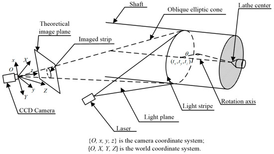
Figure 2.
Diameter measurement with the line structured light vision.
Oblique elliptic cone with ellipse of Equation (1) as the base and the camera optical center as the top can be expressed as:
When the object surface is not parallel to the image plane, distance from each point on the object surface to the image plane is different. If the attitude of the object surface relative to the image plane is mastered in the imaging space (i.e., the camera coordinate system), we can know the influence of projection distortion on shaft diameter measurement. From mathematics, in the camera coordinate system, the position of the light plane relative to the image plane is determined by the coordinates of the ellipse center and the normal vector of the light plane. Therefore, the normal vector of the light plane is used to determine the transformation relationship between the world coordinates and the camera coordinates (see Appendix A). The world coordinates of Equation (2) are transformed into the camera coordinates by and written into matrix form:
where .
After the transformation matrix is multiplied by the coefficient matrix, the above formula is expressed as:
The specific expressions of each parameter in the matrix are shown in Appendix B. Equation (4) represents an oblique elliptic cone with the ellipse formed by the intersection of the optical plane and the shaft surface as the base and the optical center of the camera as the top. Therefore, according to the principle of pinhole imaging, simultaneous Equation (4) and equation can obtain the expression of the intersection line between the light plane and the shaft surface on the theoretical image plane:
The coefficient of Equation (5) is only related to the measured shaft diameter (see Appendix B), that is, Equation (5) has only one unknown quantity. The measured shaft diameter can be obtained by fitting Equation (5) on the theoretical image. Therefore, Equation (5) is the model of shaft diameter measurement.
3. Test and Analysis of the Shaft Diameter Measurement Model
In order to verify the correctness and accuracy of the measurement model, a special test experiment is established. The structure of the test system is shown in Figure 3. The accuracy of the measurement model is related to the accuracy of the detected measurement points and the camera calibration. The calibration accuracy of the camera’s intrinsic parameters, lens distortion parameters and external parameters can meet the requirements of vision measurement of shaft diameter [32]. Therefore, after calibrating the camera’s internal parameters and distortion parameters, the influence of the accuracy of the measurement points on the accuracy of the measurement model is tested. The models and main parameters of the equipment used for the test are shown in Table 1. Since the error of detecting the square corner points of the calibration plate image is very small [33,34], the accuracy of the measurement model is tested by the corner points of the calibration plate to reduce the influence of measurement point error on the test. When testing, the surface of the calibration plate simulates the light plane. After calibrating the intrinsic parameters of the camera, the normal vector and external parameter of the calibration plate can be obtained by the detected corner coordinates. 4 corner points on the same circle are selected near the camera main point (to reduce the lens distortion) on the calibration plate, as shown in Figure 4. The symmetrical point of the 4 points is the center of the circle. The 4 points on the same circle on the calibration plate are located in the same ellipse on the image of the calibration plate. Therefore, the pixel coordinates of the ellipse center and four measuring points can be obtained by detecting the image, and the results are shown in Table 2. Then, in Table 2, is the Z coordinate (the world coordinate) of the calibration plate.
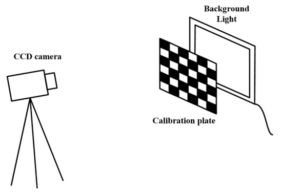
Figure 3.
The test system structure.

Table 1.
Test results of the shaft diameter measurement model (mm).
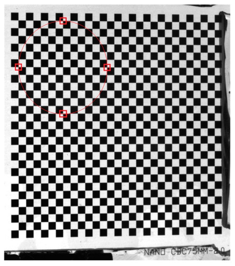
Figure 4.
Four corner points on the same circle on the calibration plate.
Table 2.
Results of the calibration and detection.
According to the principle of least squares [35,36,37,38,39], the geometric fitting of the measurement model of Equation (5) is carried out by the data in Table 2, as shown in Equation (6).
where () are the coordinates of the detected corner points; () are the coordinates of the points which are both on the ellipse and perpendicular to the point ().
The diameter of the circle, where the four points on the calibration plate is located, is obtained by optimizing Equation (6) using least squares geometric fitting [40,41,42]. In the experiment, two different known diameters determined by the grid size between the four corner points are selected as exact values for measurement, and the measurement experiment is repeated for 10 times to ensure the effectiveness. In order to verify the stability of the measurement method, change the position of the camera arbitrarily to test again. The position of the original camera is named position 1, and the changed camera position is named position 2. The diameter obtained by the optimizing is compared with the diameter determined by the grid size between the four corner points, as shown in Table 3 and Table 4. The data in Table 3 and Table 4 show that: the measurement model is correct, which can solve the influence of the projection distortion on the measurement and if the accuracy of the detected points is good, the measurement model has high measurement accuracy.
Table 3.
Test results of the shaft diameter measurement model (mm) (Position 1).
Table 4.
Test results of the shaft diameter measurement model (mm) (Position 2).
On a CA6140 lathe, the measurement accuracy of Equation (5) is tested by measuring the shafts with different diameters, as shown in Figure 5. The measured shafts were installed between the three-jaw chuck and the top of the lathe. The camera is the same as the front test. The laser line source is LH650-80-3. The equation of the connection line between the three-jaw chuck and the top and the optical plane equation are calibrated by Liu and co-workers’ method [21], the connection line equation calibration system structure is shown in Figure 6a, the optical plane equation calibration system structure is shown in Figure 6b. The normal vector of the optical plane in the camera coordinate system is obtained by the optical plane equation calibrated. Because the intersection line between the optical plane and the surface of the measured shaft is an ellipse, the coordinate of the ellipse center can be obtained by the optical plane equation and the equation of the connection line between the three-jaw chuck and the top. The coordinate transformation relationship is determined by the normal vector of the optical plane and the equation of the connection line between the three-jaw chuck and the top (see Table A1 and Equation (A13) in Appendix C).

Figure 5.
Test of the measurement model on a lathe.
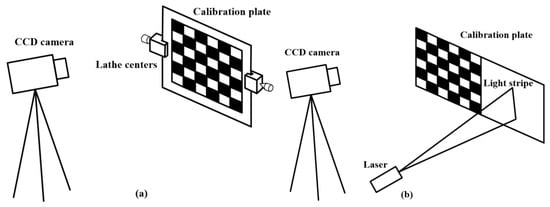
Figure 6.
The calibration system structure: (a) The calibration of the connection line equation of lathe centers; (b) The optical plane equation calibration.
As shown in Figure 7, (a) and (b) are the images of the light stripe on the shaft surface when the shaft does not rotate and it rotates, respectively. The midpoints of the light stripe images in Figure 7a are detected by the Steger method [43,44,45]. Moreover, the pixel coordinates of the detected midpoints are converted into theoretical image coordinates. The measurement accuracy of Equation (5) is tested by the theoretical image coordinates when the measured shaft does not rotate. Similarly, when the measured shaft rotates, the measurement accuracy of Equation (5) is tested by detecting the midpoint of the light stripe image in Figure 7b. The fit result of an ellipse on the theoretical image plane is shown in Figure 8. In addition, to ensure the validity of the experiment and the rigor of the research, each test is repeated 10 times, the final measurement results of three different shaft diameters are shown in Table 5. In Table 5, the roughness of the shaft is the average of three measurement values obtained by the roughness measuring instrument (TR200), and the known values of the shaft diameters are obtained by the micrometer measurement. The accuracy of the micrometer is 0.001 mm, and the average value of three measurement results of the micrometer is taken as the known value. The measured values in Table 5 are the average values of repeated measurements.
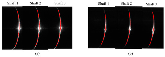
Figure 7.
The tested images on the lathe: (a) The light strip images on the shaft surfaces when the shaft speed n = 0; (b) The light strip images on the surface of the shaft when the shaft rotates.
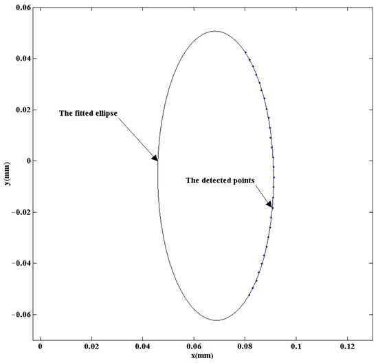
Figure 8.
Fit result of an ellipse on the theoretical image plane.
Table 5.
The final measurement results of three shaft diameters on the lathe (mm).
The data in Table 5 show that the measurement model Equation (5) is correct, and the measurement results meet the requirement, so in-situ and on-line measurement of shaft diameter can be realized by this method. However, compared with Table 3 and Table 4, the measurement error increases, this is because the precision of the calibration plate is 1 µm, the error of detecting the midpoints of the light strip image is larger than the error of detecting the square corner points of the calibration plate image. In addition, when the surface roughness of the shaft is large, there is less specular reflection and more diffuse reflection [46]. When the rotation speed of the shaft becomes higher, this situation will be aggravated, which cause the image quality of the light stripe on the rotating shaft surface is worse than that on the stationary shaft surface, so that the measurement error of rotating shaft is larger than that of static shaft.
4. Conclusions
This paper studies the measurement of shaft diameter with the structured light system composed of a laser linear light source and a camera, which can realize the in-situ and on-line measurement of shaft diameter. Based on the ellipse formed by the intersection of the light plane and the surface of the measured shaft, the measurement model of shaft diameter is established on the theoretical image plane. The measured shaft diameter can be obtained by optimizing the measurement model with the detected points on the ellipse. The measurement model requires axis of the measured shaft to be unchanged in the position of the machine tool, and general processing machine tools meet this requirement. The experimental results show that the measurement errors of three shafts with different shaft diameters at different speeds are 0.11–0.19 mm, so the measurement model of shaft diameter is accurate, and the measurement accuracy is high, which meets the engineering requirement. Compared with the existing vision measurement technology of the shaft diameter, the measurement method not only solve the influence of the projection distortion on the measurement, but also has good universality, that is, as long as the measurement shape on the laser plane is an ellipse (or a circle, which is the special shape of the ellipse), the measurement method is applicable.
If the detected points have higher accuracy, such as the precision of detecting the square corner points on the calibration plate, the measurement accuracy of the measurement model can be higher. The main factor affecting the measurement accuracy of the model is the error of the detected points on the ellipse, and the error is mainly affected by the surface roughness and the rotation speed of the shaft. Therefore, based on this measurement model, if a higher-precision measurement of the shaft diameter is required, to study the influence law of shaft surface roughness and rotation speed on the detection accuracy of the light stripe center is a desirable research direction.
Author Contributions
Methodology, Q.T. and J.M.; software, J.M. and S.L.; validation, Y.K. and B.C.; investigation, S.L. and B.C.; data curation, Y.K.; writing—original draft preparation, Q.T. and Y.K.; writing—review and editing, Q.T. and J.M.; supervision, Q.T. and J.M. All authors have read and agreed to the published version of the manuscript.
Funding
This research was funded by “Thirteenth Five-Year” Science and Technology Project of Jilin Province Education Department, grant number JJKH20200959KJ; the National Natural Science Foundation of China, grant number 52005213; 2020 Department of Human Resources and Social Security of Jilin Province Postdoctoral Researcher Selected Funding Project, grant number KF204039 and China Postdoctoral Science Foundation Funded Project, grant number 2018M641776.
Institutional Review Board Statement
Not applicable.
Informed Consent Statement
Not applicable.
Data Availability Statement
The data presented in this study are available on request from the corresponding author.
Acknowledgments
The authors are grateful to the editors and the anonymous reviewers for providing us with insightful comments and suggestions throughout the revision process.
Conflicts of Interest
The authors declare no conflict of interest.
Appendix A
Normal vector of the light plane can be obtained by the calibration board. So, the equation of the light plane is expressed as:
Firstly, the direction cosine of the Z axis of the world coordinate system in the camera coordinate system is determined by the normal vector of the light plane:
Then, the equation of the connection line between the three-jaw chuck and the top of a lathe is obtained by the calibration of using the device and method [21] in the camera coordinate system.
In the planes passing through the connection line between the three-jaw chuck and the top, one plane is perpendicular to the light plane, and according to the point product of the normal vectors of the two planes is 0, the plane is obtained:
where .
The equation of the intersection line between the plane of Equation (A4) and the light plane is:
According to Equation (A5), the direction cosine of the X axis of the world coordinate system in the camera coordinate system is:
where .
Finally, the direction cosine of the Y axis in the camera coordinate system is obtained by cross product of the direction numbers of the Z axis and X axis according to the right-hand rule.
where .
The transformation relationship between the world coordinate and the camera coordinate is obtained by Equations (A2), (A6) and (A7).
where the lower case letter is the camera coordinate, and the capital letter is the world coordinate.
Therefore, the transformation matrix is:
When the four corner points on the calibration board in Figure 4 are used for the test, the transformation matrix is:
Because the measured shaft is installed between the three-jaw chuck and the top of the lathe, the coordinates (tx0, ty0, tz0) of center of the ellipse formed by the intersection line between the light plane and the measured shaft surface can be obtained by Equation (A1) and Equation (A3). Therefore, in the world coordinate system, the center of the ellipse is represented:
Appendix B
The coefficients in Equation (4) are:
Appendix C
Table A1.
The measurement results of the shaft diameters on the lathe (mm).
Table A1.
The measurement results of the shaft diameters on the lathe (mm).
| 6803.90 | 6803.78 | 2.51 | 640.12 | 480.10 | 0.02 | 19.42 | 0.0004 | −0.0001 |
| The Normal Vector and External Parameter of the Structured Light | ||||||||
| −0.002618 | −0.000139 | −0.001077 | 15.39 | −4.55 | 891.46 | |||
References
- Zhang, Z.; Liu, Y.; Hu, Q.; Zhang, Z.; Wang, L.; Liu, X.; Xia, X. Multi-information online detection of coal quality based on machine vision. Powder Technol. 2020, 374, 250–262. [Google Scholar] [CrossRef]
- Sun, W.; Yeh, S. Using the Machine Vision Method to Develop an On-machine Insert Condition Monitoring System for Computer Numerical Control Turning Machine Tools. Materials 2018, 11, 1977. [Google Scholar] [CrossRef] [PubMed]
- Makela, M.; Rissanen, M.; Sixta, H. Machine vision estimates the polyester content in recyclable waste textiles. Resour. Conserv. Recycl. 2020, 161. [Google Scholar] [CrossRef]
- Jones, J.; Foster, W.; Twomey, C.; Burdge, J.; Ahmed, O.; Pereira, T.; Wojick, J.; Corder, G.; Plotkin, J.; Abdus-Saboor, I. A machine-vision approach for automated pain measurement at millisecond timescales. eLife 2020, 9. [Google Scholar] [CrossRef] [PubMed]
- Sun, X.; Xu, S.; Lu, H. Non-Destructive Identification and Estimation of Granulation in Honey Pomelo Using Visible and Near-Infrared Transmittance Spectroscopy Combined with Machine Vision Technology. Appl. Sci. 2020, 10, 5399. [Google Scholar] [CrossRef]
- Viejo, C.; Fuentes, S.; Howell, K.; Torrico, D.; Dunshea, F. Robotics and computer vision techniques combined with non-invasive consumer biometrics to assess quality traits from beer foamability using machine learning: A potential for artificial intelligence applications. Food Control 2018, 92, 72–79. [Google Scholar] [CrossRef]
- Zhang, Z.; Wang, X.; Zhao, H.; Ren, T.; Xu, Z.; Luo, Y. The Machine Vision Measurement Module of the Modularized Flexible Precision Assembly Station for Assembly of Micro- and Meso-Sized Parts. Micromachines 2020, 11, 918. [Google Scholar] [CrossRef]
- Li, W.; Jin, J.; Li, X.; Li, B. Method of rotation angle measurement in machine vision based on calibration pattern with spot array. Appl. Opt. 2010, 49, 1001–1006. [Google Scholar] [CrossRef]
- Lian, F.; Tan, Q.; Liu, S. Block Thickness Measurement of Using the Structured Light Vision. Int. J. Pattern Recognit. Artif. Intell. 2019, 33. [Google Scholar] [CrossRef]
- Chen, J.; Jing, L.; Hong, T.; Liu, H.; Glowacz, A. Research on a Sliding Detection Method for an Elevator Traction Wheel Based on Machine Vision. Symmetry 2020, 12, 1158. [Google Scholar] [CrossRef]
- Shen, H.; Li, S.; Gu, D.; Chang, H. Bearing defect inspection based on machine vision. Measurement 2012, 45, 719–733. [Google Scholar] [CrossRef]
- Moru, D.; Borro, D. A machine vision algorithm for quality control inspection of gears. Int. J. Adv. Manuf. Technol. 2019, 106, 105–123. [Google Scholar] [CrossRef]
- Wu, F.; Mao, J.; Zhou, Y.; Qing, L. Three-line structured light measurement system and its application in ball diameter measurement. Optik 2018, 157, 222–229. [Google Scholar] [CrossRef]
- Bao, H.; Tan, Q.; Liu, S.; Miao, J. Computer Vision Measurement of Pointer Meter Readings Based on Inverse Perspective Mapping. Appl. Sci. 2019, 9, 3729. [Google Scholar] [CrossRef]
- Guo, S.; Zhang, J.; Jiang, X.; Peng, Y.; Wang, L. Mini milling cutter measurement based on machine vision. Procedia Eng. 2011, 15, 1807–1811. [Google Scholar]
- Gao, L.; Wang, Z.; Liu, Y.; Guo, J.; Liu, C. Vision measurement technique of axle based on double beam. Optik 2018, 174, 757–765. [Google Scholar] [CrossRef]
- Wei, G.; Tan, Q. Measurement of shaft diameters by machine vision. Appl. Opt. 2011, 50, 3246–3253. [Google Scholar] [CrossRef]
- Sun, Q.; Hou, Y.; Tan, Q.; Li, C. Shaft diameter measurement using a digital image. Opt. Laser Eng. 2014, 55, 183–188. [Google Scholar] [CrossRef]
- Li, B. Research on geometric dimension measurement system of shaft parts based on machine vision. EURASIP J. Image Video Process. 2018, 10. [Google Scholar] [CrossRef]
- Che, J.; Ratnam, M. Real-time monitoring of workpiece diameter during turning by vision method. Measurement 2018, 126, 369–377. [Google Scholar] [CrossRef]
- Liu, S.; Tan, Q.; Zhang, Y. Shaft Diameter Measurement Using Structured Light Vision. Sensors 2015, 15, 19750–19767. [Google Scholar] [CrossRef] [PubMed]
- Liu, W.; Jia, Z.; Wang, F.; Ma, X.; Wang, W.; Jia, X.; Song, D. An improved online dimensional measurement method of large hot cylindrical forging. Measurement 2012, 45, 2041–2205. [Google Scholar] [CrossRef]
- Wu, B.; Xue, T.; Zhang, T.; Ye, S. A novel method for round steel measurement with a multi-line structured light vision sensor. Meas. Sci. Technol. 2010, 21, 025204. [Google Scholar] [CrossRef]
- Liu, B.; Wang, P.; Zeng, Y.; Sun, C. Measuring method for micro-diameter based on structured-light vision technology. Chin. Opt. Lett. 2010, 8, 666–669. [Google Scholar]
- Gong, Z.; Sun, J.; Zhang, G. Dynamic Measurement for the Diameter of a Train Wheel Based on Structured-Light Vision. Sensors 2016, 16, 564. [Google Scholar] [CrossRef] [PubMed]
- Zhang, Y.; Liu, W.; Lu, Y.; Cheng, X.; Luo, W.; Di, H.; Wang, F. Accurate profile measurement method for industrial stereo-vision systems. Sens. Rev. 2020, 40, 445–453. [Google Scholar] [CrossRef]
- Malyarchuk, V.; Jung, I.; Rogers, J.; Shin, G.; Ha, J. Experimental and modeling studies of imaging with curvilinear electronic eye cameras. Opt. Express 2010, 18, 27346–27358. [Google Scholar] [CrossRef]
- Zhang, G.; Wei, Z. A position-distortion model of ellipse centre for perspective projection. Meas. Sci. Technol. 2003, 14, 1420–1426. [Google Scholar] [CrossRef]
- Li, Z.; Zgadzaj, R.; Wang, X.; Reed, S.; Dong, P.; Downer, M. Frequency-domain streak camera for ultrafast imaging of evolving light-velocity objects. Opt. Lett. 2010, 35, 4087–4089. [Google Scholar] [CrossRef]
- Zhang, Z.; Zhao, R.; Liu, E.; Yan, K.; Ma, Y. A single-image linear calibration method for camera. Measurement 2018, 130, 298–305. [Google Scholar] [CrossRef]
- Lv, B.; Li, L.; Yan, C. Three-dimensional laser scanning under the pinhole camera with lens distortion. In Proceedings of the 4th IEEE International Conference on Cloud Computing and Intelligence Systems (IEEE CCIS), Beijing, China, 17–19 August 2016; Volume 28, pp. 737–742. [Google Scholar]
- Zhang, Z. A flexible new technique for camera calibration. IEEE Trans. Pattern Anal. Mach. Intell. 2000, 22, 1330–1334. [Google Scholar] [CrossRef]
- Bouguet, J.Y. Pyramidal Implementation of the Lucas Kanade Feature Tracker Description of the Algorithm; Technical Report; OpenCV Document. Intel Microprocessor Research Labs: Santa Clara, CA, USA, 2000. [Google Scholar]
- Bouguet, J.Y. Camera Calibration Toolbox for Matlab. Available online: https://www.vision.caltech.edu/bouguetj/calib_doc/index.html (accessed on 5 June 2020).
- Markovsky, I.; Kukush, A.; Van Huffel, S. Consistent least squares fitting of ellipsoids. Numer. Math. 2004, 98, 177–194. [Google Scholar] [CrossRef]
- Mortari, D. Least-Squares Solution of Linear Differential Equations. Mathematics 2017, 5, 48. [Google Scholar] [CrossRef]
- Mirzaei, D. Direct approximation on spheres using generalized moving least squares. BIT Numer. Math. 2017, 57, 1041–1063. [Google Scholar] [CrossRef]
- Bos, L.; Sommariva, A.; Vianello, M. Least-squares polynomial approximation on weakly admissible meshes: Disk and triangls. J. Comput. Appl. Math. 2010, 235, 660–668. [Google Scholar] [CrossRef]
- Liang, W.; Chapman, C.; Frisch, M.; Li, X. Geometry Optimization with Multilayer Methods Using Least-Squares Minimization. J. Chem. Theory Comput. 2010, 6, 3352–3357. [Google Scholar] [CrossRef]
- Ahn, S.; Rauh, W.; Warnecke, H. Least-squares orthogonal distances fitting of circle, sphere, ellipse, hyperbola, and parabola. Pattern Recognit. 2001, 34, 2283–2303. [Google Scholar] [CrossRef]
- Fitzgibbon, A.; Pilu, M.; Fisher, R. Direct least square fitting of ellipses. IEEE Trans. Pattern Anal. Mach. Intell. 1999, 21, 476–480. [Google Scholar] [CrossRef]
- Ahn, S.; Rauh, W. Geometric least squares fitting of circle and ellipse. Int. J. Pattern Recognit. Artif. Intell. 1999, 13, 987–996. [Google Scholar] [CrossRef]
- Steger, C. An unbiased detector of curvilinear structures. IEEE Trans. Pattern Anal. Mach. Intell. 1998, 20, 113–125. [Google Scholar] [CrossRef]
- Qi, L.; Zhang, Y.; Zhang, X.; Wang, S.; Xie, F. Statistical behavior analysis and precision optimization for the laser stripe center detector based on Steger’s algorithm. Opt. Express 2013, 21, 13442–13449. [Google Scholar] [CrossRef] [PubMed]
- Wang, W.; Liang, Y. Rock Fracture Centerline Extraction based on Hessian Matrix and Steger algorithm. KSII Trans. Internet Inf. Syst. 2015, 9, 5073–5086. [Google Scholar]
- Stainvas, I.; Lowe, D. A generative model for separating illumination and reflectance from images. J. Mach. Learn. Res. 2004, 4, 1499–1519. [Google Scholar]


Publisher’s Note: MDPI stays neutral with regard to jurisdictional claims in published maps and institutional affiliations. |
© 2021 by the authors. Licensee MDPI, Basel, Switzerland. This article is an open access article distributed under the terms and conditions of the Creative Commons Attribution (CC BY) license (http://creativecommons.org/licenses/by/4.0/).