Abstract
This study proposes a parallel six-axis force/torque sensor decoupling method based on an independent component analysis (ICA), and the experimental platform is built for experimental exploration. First of all, the structural model and mathematical model of the parallel six-axis force/torque sensor are introduced, which is composed of single-dimensional force sensors with central symmetry. Secondly, the test prototype was developed and a test platform was built to perform online static loading test on the sensor, and the test results were analyzed. Finally, the ICA-based dynamic decoupling study of the sensor is carried out, the effectiveness and rationality of the proposed algorithm are proved. The research results of this paper have certain reference values for the further study of the decoupling of parallel six-axis force/torque sensors.
1. Introduction
With the development of sensing technology and computer technology, robots have a higher level of intelligence and better ability to interact with people [1,2]. In the industry of the robot, people’s requirements for signal detection and intelligent control are intensifying [3]. Six-axis force/torque sensors are often installed at the wrist of the robot to force the working state of the robot. Many strain elements of six-axis force/torque sensors are symmetrical. Since the six-axis force/torque sensor is powerful, compact, and small, the problem of coupling between dimensions is a common problem [4,5,6]. The key issue in making six-axis force/torque sensors accurate is to eliminate the coupling between dimensions, which is an extremely important prerequisite for robots to achieve intelligent control.
Decoupling studies on sensors often require calibration before they are used, so better calibration methods have a significant impact on the accuracy performance of the sensor [7,8,9]. The least squares method is the most commonly used calibration method so far because of its intuitive characteristics, accuracy and because it is easy to test [10,11]. As an alternative to the least squares method, Richard M. Voyles proposed the SFM calibration method [12]. This method is based on the “shape and motion decomposition” technique of computer vision (Tomasi and Kanade, 1991). Unlike the least-squares technique, the shape from the motion calibration does not require knowledge of the resolution of all interventions. Instead, it uses a very large amount of raw output that is easily available, with some scholars having verified the accuracy of the calibration method [13]. In 2015, Danfeng Chen [14] designed a large-range six-axis force/torque sensor applied to the space manipulator and calibrated it.
In the research of six-axis force/torque sensor decoupling, Guo [15] explored a local structure decoupling method (LSDM), which can achieve decoupling of translation and rotation in a short time. Hayward explored three parallel decoupling mechanisms through geometric analysis with less freedom to implement different types of decoupling motions [16]. Wang [17] used a calibration matrix to eliminate mutual coupling and proposed an experimental study of the best design and fully prestressed six-axis force/torque sensor. The Last Square Support Vector Machine Regression (LSSVR) is applied to the sensor decoupling in the study of Li. The maximum non-linear error and cross-coupling error of the sensor after decoupling are 0.89% and 0.1%. Jia [18] proposed a method for decoupling the force/torque stiffness of the six-axis force sensor. In this method, the condition of force/torque stiffness decoupling is analyzed, and the relationship between stiffness decoupling and elastic limb posture is established. The results show that the six-axis force sensor designed by this method has low error and provides reliable design guidance for the design of decoupling six-axis force sensor. Yao et al. [19] studied the isotropy performance of sensors and obtained the analytic relations of key structural parameters leading to isotropic configuration.
Although force sensors have been widely used in many fields, there are still few studies on dynamic decoupling of sensors. An important issue that needs to be solved by the six-axis force/torque sensor is coupling. Since the six-axis force/torque sensor has an integrated elastomer structure and there might be errors in the installation process, the sensor has coupling between the switching channels in different directions. This situation seriously affects the measurement accuracy of the sensor, so the decoupling analysis of the six-axis force/torque sensor is very important. At present, most decoupling is based on a modeling or decoupling network design, which is computationally complex and cannot establish the exact model of some complex systems at all. Using an independent component analysis (ICA) to decouple the sensor requires less calculation and more accurate data processing. ICA has not been applied to the decoupling research of six-axis force/torque sensors, so the use of ICA for decoupling research can fill the gap in this regard.
Based on the above facts, ICA is used to study the decoupling of sensors. ICA is an analysis method based on the high-order statistical characteristics of signals. The signal between the sensor channels is non-Gaussian and the components are independent on each other. Because of this characteristic, ICA can be used as a decoupling algorithm to meet the actual situation. In this paper, a decoupling method for parallel six-axis force/torque sensor based on ICA is proposed and experimentally studied. The purpose is that the output of the six-axis force/torque sensor after static/dynamic decoupling can meet the requirements, and can quickly and accurately respond to changes in the measured data.
The remainder of this paper is organized as follows. The structural model and mathematical model of the sensor are given in Section 2. Section 3 describes how we carried out the loading test on the sensor prototype and analyzed the results. The decoupling study of the ICA method for sensors is detailed in Section 4. Finally, Section 5 contains a summary of this paper.
2. Parallel Six-Axis Force/Torque Sensor
This section mainly describes the analysis of the mathematical model and sensor prototype of the six-axis force/torque sensor.
2.1. Introduction to Parallel Six-Axis Force/Torque Sensor Structure
Many factors must be considered in the development of the sensor prototype, such as the strength and stiffness of the entire structure and whether its layout is reasonable. The range design of the six-axis force/torque sensor is as follows: , . The measurement branch is an S-type one-dimensional force sensor with a measuring range of 5 kg. The material of the measuring branch is selected from alloy steel, and its properties are defined as follows: density , elastic modulus , Poisson’s ratio .
The measurement branch is shown in Figure 1. The S-type force sensor is a closed quadrilateral steel frame that uses the S-curve path to complete the force transmission.
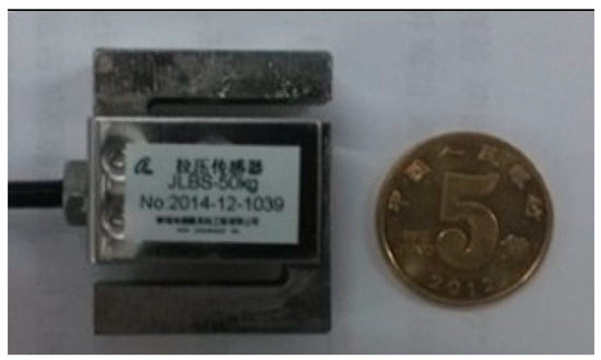
Figure 1.
S type single-dimensional force sensor.
The strain beam structure is located in the middle of the S-type sensor, and the double-bend beam structure used in this paper greatly reduces the overall volume of the sensor and has the advantages of easy processing. The working principle of the strain gauge is that when the S-type sensor is subjected to an external force, its resistance value will change accordingly. Therefore, the strain gauge should be installed at the weakest part of the top of the middle hole. The thickness of the upper and lower beams of the middle hole of the sensor is relatively thin, while the rest is thicker. The thickness of the strain gauge mounting position can be increased by enlarging the distance of the hole, and the rigidity thereof is also greatly improved. A prototype of an orthogonal parallel six-axis force/torque sensor assembled by the upper and lower platforms and the measuring branch is shown in Figure 2, with an overall thickness of 15 mm. The range is 5 kg and the external dimensions are 30 × 20 × 10 mm. Both the force measuring platform and the fixed platform are hexagons with a diameter of 50 mm and a thickness of 8 mm, while the thickness of the column is 6 mm.
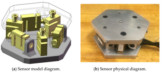
Figure 2.
Six-axis force/torque sensor.
2.2. Mathematical Model of Parallel Six-Axis Force/Torque Sensor
The schematic diagram of the structure of an orthogonal parallel six-axis force/torque sensor is shown in Figure 3.
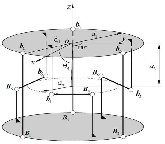
Figure 3.
Orthogonal parallel six-axis force/torque sensor.
Such sensors are composed of six identical measurement branches, a load platform ( are three fixed points above the force platform, respectively) and a fixed platform ( are three fixed points above the fixed platform; the two platforms are identical and have a radius of . The distance between the geometric centers of the two platforms is ). are three vertically distributed measurement branches, where the angle between any two points of and the origin O is ; are three horizontally distributed measurement branches and are tangent to a circle of radius . These three tangent points are not only uniformly distributed on the circumference, but also the midpoint of the horizontal measurement branch. The measurement reference coordinate system of the sensor is a Cartesian coordinate system, and the origin is determined as the geometric distribution center of the force measurement platform. The z-axis is not only parallel to the vertical measuring branch but also perpendicular to the fixed platform and oriented upwards. The distance between the force measuring platform and the horizontal measuring branch is .
The static equilibrium equation of the force platform is established as follows:
where is a spatial three-dimensional external force and a spatial three-dimensional external torque vector acting on the force measuring platform; is a matrix of mapping coefficients between the axial force and the six-dimensional external force of the six measuring branches; represents six measuring branch axial force vectors.
The first-order mapping coefficient matrix in Equation (1) is as follows:
where:
—the angle between and -axis;
—the angle between the midpoint of and the -axis;
—the radius length of force platform;
—the inscribed circle radius length;
—the vertical distance between the force measurement platform and the inscribed circle;
—the vertical distance between the upper and lower platforms.
Thus, we can get the following formula:
where represents the mapping relationship between the force platform and the reaction force of the measuring branch under the force of six dimensions in space.
3. Online Static Loading Test
This section mainly builds a calibration test system, conducts calibration tests on sensors, and analyzes the coupling between sensor dimensions.
3.1. Introduction to Test System and Loading Method
The online static loading test consists of two parts: a hardware system and software system. Among them, the hardware system includes sensor prototype, voltage signal amplifier, computer, DC power supply, weight, and data acquisition card, which are shown in Figure 4. The data acquisition card uses PCI8932, its AD analog input function is mainly used. AD conversion function can realize the conversion from analog to digital. The main parameters are shown in Table 1.
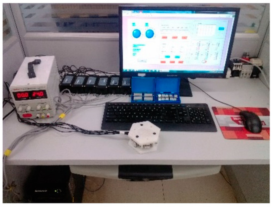
Figure 4.
Hardware system.

Table 1.
AD analog main parameters.
In order to achieve the purpose of improving the accuracy of the loading force, this test uses a 0.5 kg standard weight with an accuracy level of M1. Figure 5 shows the AD acquisition flow chart in the software system, and Figure 6 shows the front panel of the online static loading software system based on LabVIEW.
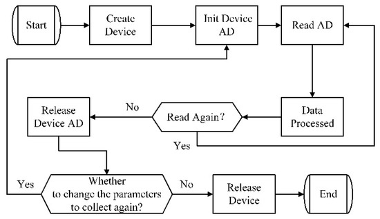
Figure 5.
The flow chart of the AD collection.
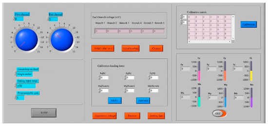
Figure 6.
Front panel.
The choice of coordinate system will have an impact on the entire static calibration test. The sensor is in direct contact with the end of the manipulator. The six-axis force/torque sensor is installed at the end of the robot for static calibration in order to reduce the influence of gravity on the sensor during the loading process. The two loading points about the origin symmetry are at the edge of the force measurement platform, establishing the positive and negative directions of the x-axis. The change of the sensor pose is adjusted by adjusting the pose of the robot. The loading points in the three directions of x, y, z in turn add weights starting from 0 and incremented by each time until it reaches a load of .
3.2. Analysis of Loading Test Results
The specific steps for static calibration are as follows:
- Adjust the arm position to the position where the sensor is loaded, adjust the DC voltage to 24 V, and run the software to reset the initial voltage.
- Perform 20 load and unload tests in sequence at the load point and store the voltage of each load point in turn.
- Perform a calibration test on the prototype according to steps (1) and (2) and save the test data to Excel.
- Check and test the test data, calculate the matrix of the fit coefficient, and determine the static performance index.
The equation of the mapping relationship between the loaded calibration force/torque and the branch output voltage can be expressed as:
where is the force of Space six-dimensional calibration; is the output voltage of the measuring limb measure branch; is the mapping matrix between the calibration force and the output voltage of the measurement branch.
After applying the calibration force 20 times to the six-dimensional force sensor, the matrix of the corresponding measured branch output voltage, , is obtained, and when the number of measurement branches is n, the output voltage matrix is of an order. The pseudo-inverse matrix of the output voltage matrix of the measurement branch is multiplied to the left and right sides of Equation (5), which can be obtained as:
where is the pseudo inverse matrix of ; ; is the calibration matrix.
The loaded experimental data is brought into Equation (6). After the least square test data processing, the calibration matrix shown in Equation (7) can be obtained:
Based on previous research [20], we know that the measured value of the sensor’s calibration force can be expressed as:
where , with each of these being a dimensional matrix, m is the number of loading points with m = 6, is the calibration force matrix, is the matrix of the corresponding measured branch output voltage, and is the pseudo inverse matrix of .
The difference was determined between the actual and calculated values of the calibration force and the absolute value was taken, after which we obtained the deviation matrix, which can be expressed as:
The ratio of the average value of the deviation of each item of Equation (9) to the full-load calibration force or the calibration torque in the corresponding measurement direction is defined as the linearity of the sensor in the actual measurement. For example, the calculation formula of the force linearity vector in the x direction can be expressed as:
where is the ith row element of matrix and is the average of all the elements in vector . and is the full-load calibration force/moment in that direction.
In Equation (8), the first term of vector reflects the linearity of the x-measurement direction when the x-direction calibration force is loaded, and the other five terms reflect the coupling linearity of the remaining five dimensions when the x-direction calibration force is applied.
Similarly, the linearity and coupling degree of the other five-dimensional calibration force/torque can be calculated. The linearity matrix of the sensor can be expressed as:
The data in Equation (5) is processed according to Equations (6)–(9), and the linearity matrix of the prototype can be expressed as:
It can be seen from Equation (12) that the maximum inter-dimensional coupling of the sensor is 7.99%. As such, the sensor has a relevant coupling factor; thus, there is a need to dynamically decouple the sensor to ensure that the sensor has a good dynamic response accuracy.
4. Dynamic Decoupling Research of Parallel Six-Axis Force/Torque Sensor
This section mainly describes the research on the dynamic decoupling of sensors. The output after ICA decoupling is compared with the output after the diagonal dominance matrix is decoupled to highlight the advantages of this research work.
4.1. Dynamic Decoupling Based on Diagonal Dominant Matrices (DDM)
A six-axis force/torque sensor needs to respond quickly and accurately to changes in the measured data. Therefore, the sensor must be dynamically decoupled to meet the application requirements. The transfer function of the parallel six-axis force/torque sensor is , the constant decoupling compensation network behind the transfer function is , and the transfer function of the parallel six-axis force/torque sensor is represented by . The basic idea of this decoupling method is to make the sum of the absolute values of the non-diagonal elements in each row of smaller than the diagonal elements to achieve the diagonal advantage of the matrix [21].
The existing diagonal dominance matrix method is used to dynamically decouple the sensor in order to reflect its decoupling effect. The unit step input signals are then loaded onto channels 1, 2, and 3, respectively, and the corresponding output signals, as shown in Figure 7 and Figure 8, can be obtained.
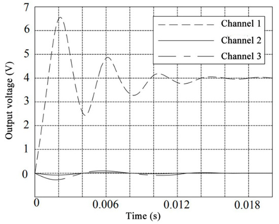
Figure 7.
Channel 1 output.
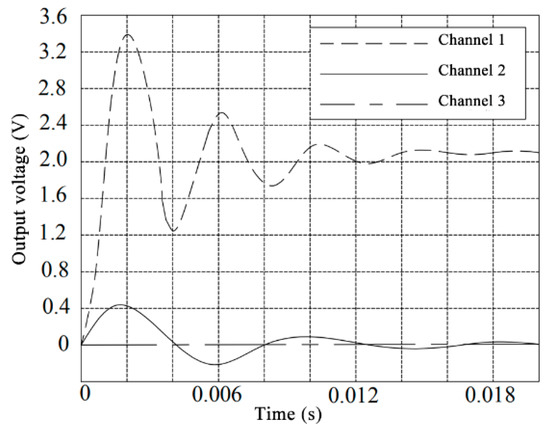
Figure 8.
Channel 1 output after DDM.
The output after applying the unit step signal to channel 2 is as shown in Figure 9. The output after decoupling through the DDM is shown in Figure 10. The output after applying the unit step signal to the channel 3 is shown in Figure 11, and the output after decoupling through the DDM is shown in Figure 12.
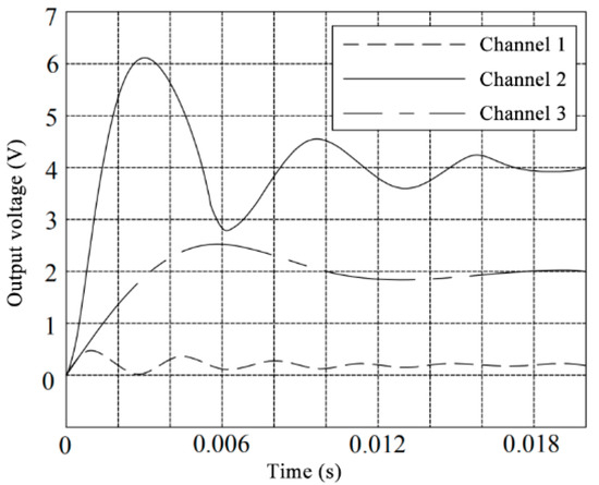
Figure 9.
Channel 2 output.
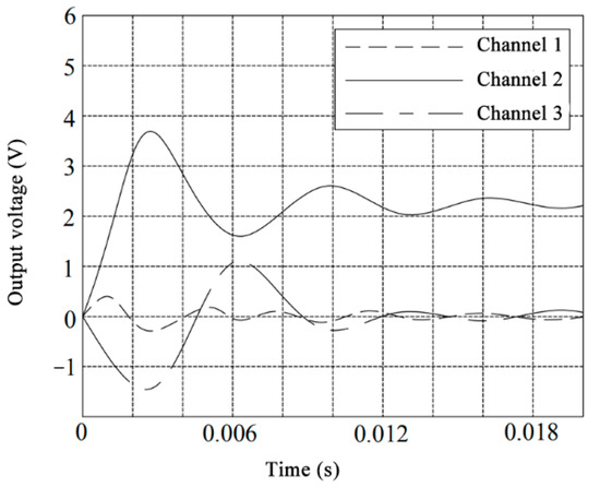
Figure 10.
Channel 2 output after DDM.
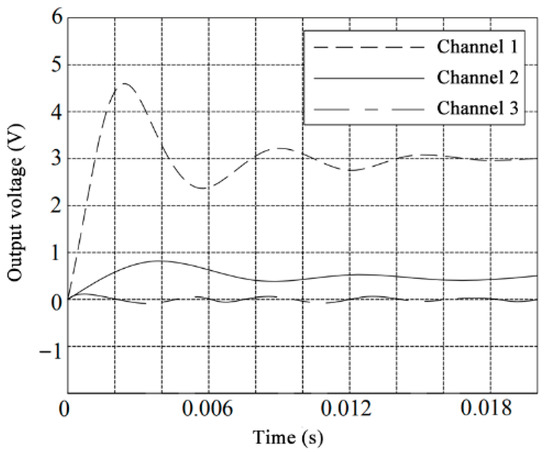
Figure 11.
Channel 3 output.
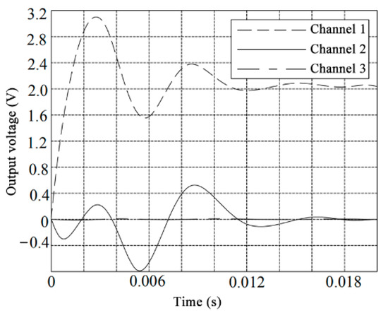
Figure 12.
Channel 3 output after DDM.
It can be seen from the above analysis that the output signal decoupled by the diagonal advantage compensation is somewhat stable, and it is finally stabilized at about 2.2 V, but the system is not fully decoupled.
4.2. Dynamic Decoupling Based on ICA
In many cases, sensors need to respond quickly and accurately to changes in measurement data. Therefore, dynamic decoupling of sensors must be studied to achieve this goal. In this section, ICA is used to decouple the sensor to make it respond more quickly and accurately to data processing. The ICA decoupling method and the traditional diagonal dominance matrix decoupling method are compared to highlight the significance of this work. ICA is a computational method and statistical technique. The process of ICA is actually optimized by establishing an objective function to achieve an approximate goal, which mathematical model is shown in Figure 13. The vector matrix model of ICA is as follows:
where X is the observed signal, with , S is the source signal, with , and A is a hybrid matrix, with .
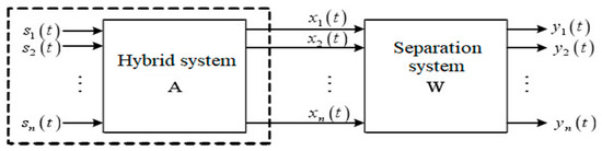
Figure 13.
ICA model.
The starting point of ICA is to assume that the source signals S are independent of each other, and establish a separation matrix W and a mixture matrix A by establishing an objective function based on independence. The source signal can be estimated by the following formula:
A complete estimation of the source signal is achieved when is established.
The ICA algorithm includes three main aspects: centralization, whitening, and independent component decomposition. The whitening matrix can be expressed as:
where . Then, we can get .
In general, the choice of the ICA algorithm is basically between the adaptive algorithm and the batch algorithm. The Fast ICA [22] algorithm is a very useful batch processing algorithm, which can be used to maximize the multi-dimensional objective function. This algorithm maximizes the negative entropy of A based on the objective function of negative entropy, which is characterized by fast convergence and robustness.
MATLAB and SIMULINK simulation functions are used to create a simulation of a parallel six-axis force/torque sensor system. The unit step input signals are, respectively, loaded onto channels 1, 2, and 3, after which we can obtain the corresponding output signals of the parallel six-axis force/torque sensor. We can then simplify the above SIMULINK simulation data (centralization and whitening, etc.) and decouple the preprocessed test data into ICA.
Channels 1, 2, and 3 are, respectively, the input with unit step signals, while the outputs decoupled by ICA are shown in Figure 14, Figure 15 and Figure 16.
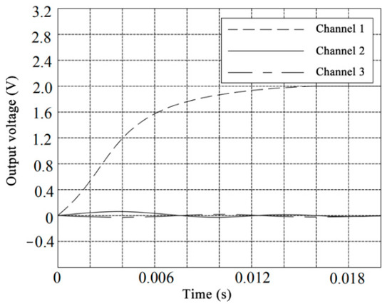
Figure 14.
The output of Channel 1 after ICA.
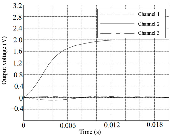
Figure 15.
The output of Channel 2 after ICA.
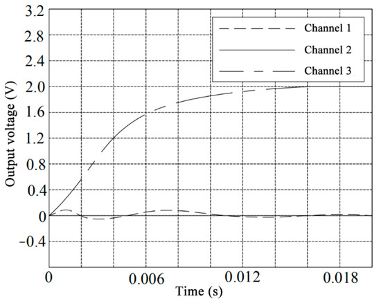
Figure 16.
The output of Channel 3 after ICA.
The unit step signal of the main channel of the sensor after the ICA is close to the ideal input, which can be derived from Figure 14, Figure 15 and Figure 16. The output of the other channels is almost equal to zero, indicating that the inter-dimensional coupling of the sensor is greatly reduced and the desired goal is achieved.
Figure 17 shows the output signal after applying the unit step signal to the three channels of the sensor simultaneously. It can be seen from Figure 17 that the output signal of the sensor oscillates before 0.01 s, and the maximum value of the oscillation is 6.4 V. After 0.02 s, the sensor output signal tends to a state of about 4 V. However, it is not completely stable, and thus, the sensor has a certain degree of inter-dimensional coupling. The output signal after dynamic decoupling of the sensor by the ICA method is shown in Figure 18. It can be seen that the output signal decoupled by the ICA method is close to the ideal unit step input after 0.014 s, and the output is at 2 V.
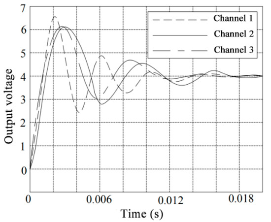
Figure 17.
The output of the sensor.
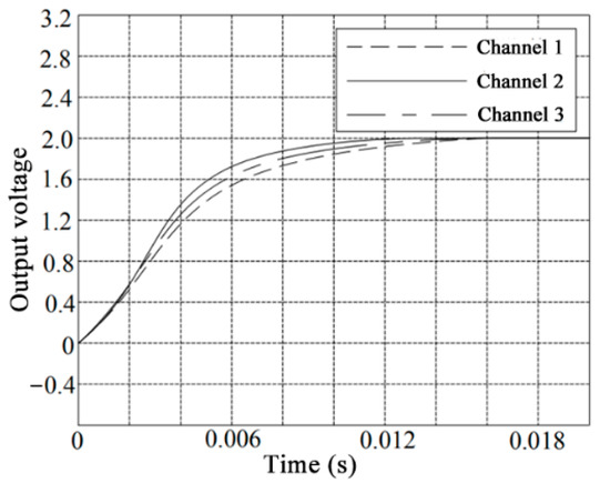
Figure 18.
The output of the sensor after ICA.
The above results prove that the coupling of the parallel six-axis force/torque sensor after decoupling with ICA is small, and the measurement accuracy is greatly improved. The use of ICA for dynamic decoupling of parallel six-axis force/torque sensors has a good application value.
4.3. Analysis of Results
The output peak value and steady-state value after decoupling of different methods are summarized in Table 2 and Table 3 in order to make a significant comparison of the output curve, where ‘None’ represents the original output signal.
Table 2.
Output of each channel.
Table 3.
Output value of each channel.
The output signal of the sensor is preprocessed (including centralization, whitening, etc.), and then the diagonal dominance matrix decoupling and ICA decoupling are performed, obtaining the decoupled output signals, as shown in Figure 8, Figure 10, Figure 12, Figure 14, Figure 15, Figure 16 and Figure 18, respectively. It can be seen from the above results, and Table 2 and Table 3, that the output after the ICA method decoupling is compared with the DDM decoupling, although there is still a certain degree of coupling in each direction, but the output of the remaining channels appears symmetrically near the 0 position, and the fluctuation range is smaller. The output stabilizes at around 2 V after 0.014 s, which is close to the ideal unit step input. The above results prove that the coupling of the parallel six-axis force/torque sensor after decoupling using independent component analysis is very small. Compared with the output of the diagonal dominance matrix decoupling, the measurement accuracy of the parallel six-axis force/torque sensor is greatly improved. This proves that ICA has a very good dynamic decoupling effect on the parallel six-axis force/torque sensor.
5. Conclusions
In this article, the mathematical model of the parallel six-axis force/torque sensor is established, and the balance relationship between the force on the force measurement platform and the force measurement branch is derived. Then, a parallel six-axis force/torque sensor was designed, with calibration research and coupling analysis carried out on it. The sensor is calibrated and the sensor is dynamically decoupled using the traditional diagonal dominance matrix decoupling and ICA decoupling methods. Finally, the traditional method and the waveform of each channel after ICA decoupling are compared, and the following conclusions can be drawn: the coupling of this sensor is smaller after independent component analysis (ICA) analysis and decoupling. Compared with the traditional diagonal dominance matrix method, the interdimensional coupling decoupled by ICA shows a certain symmetry, and the fluctuation is significantly reduced. Experimental results show that ICA can achieve fast and accurate dynamic decoupling of sensors. However, the ICA method is more complicated in practice, so it is hoped that simpler and faster methods suitable for engineering needs can be found to decouple this type of sensor. The research results of this paper provide a certain theoretical and experimental basis for improving the development of parallel six-axis force/torque sensors in various fields.
We plan to conduct research in the following areas to improve the accuracy of sensor dynamic response: (1) Apply intelligent algorithms to sensor decoupling to improve the algorithm convergence speed and improve the sensor decoupling accuracy; (2) Analyze the factors affecting the accuracy of decoupling, and propose a dynamic decoupling algorithm with a fast response speed.
Author Contributions
Methodology, Z.W. and L.L.; software, L.L.; data curation, J.H. and Z.L.; writing—original draft preparation, Z.W., L.L. and K.W.; writing—review and editing, Z.W. and L.L.; supervision, Z.W.; project administration, Z.W.; funding acquisition, Z.W. All authors have read and agreed to the published version of the manuscript.
Funding
This work is supported by the National Natural Science Foundation of China (No. 51505124), the University Science and Technology Research Project of Hebei Province (No. ZD2020151), and the Foster fund projects of the North China University of Science and Technology (No. JP201505).
Institutional Review Board Statement
Not applicable.
Informed Consent Statement
Not applicable.
Data Availability Statement
Not applicable.
Conflicts of Interest
The authors declare no conflict of interest.
References
- Gao, W.; Jia, C.; Jiang, Z.; Zhou, X.; Zhao, L.; Sun, D. The design and analysis of a novel micro force sensor based on depletion type movable gate field effect transistor. J. Microelectromech. Syst. 2019, 99, 1–13. [Google Scholar] [CrossRef]
- Stewart, R.J.; Jeon, B.S. Decoupling strength and grid resolution in peridynamic theory. J. Peridynamics Nonlocal Modeling 2019, 1, 97–106. [Google Scholar] [CrossRef]
- Li, Y.; Wang, G.; Yang, X.; Zhang, H.; Han, B.; Zhang, Y. Research on static decoupling algorithm for piezoelectric six axis force/torque sensor based on LSSVR fusion algorithm. Mech. Syst. Signal Process. 2018, 110, 509–520. [Google Scholar] [CrossRef]
- Zhao, Y.; Zhang, C.; Zhang, D.; Shi, Z.; Zhao, T. Mathematical model and calibration experiment of a large measurement range flexible joints 6-UPUR six-axis force sensor. Sensors 2016, 16, 1271. [Google Scholar] [CrossRef] [PubMed]
- Ballo, F.; Gobbi, M.; Mastinu, G. Advances in force and moments measurements by an innovative six-axis load cell. Exp. Mech. 2014, 54, 571–592. [Google Scholar] [CrossRef]
- Hogrev, S.; Tracht, K. Design and implementation of multi axial force sensing gripper fingers. Prod. Eng. Res. Devel. 2014, 8, 765–772. [Google Scholar] [CrossRef]
- Gao, Z.; Zhang, D. Design, analysis and fabrication of a multidimensional acceleration sensor based on fully decoupled compliant parallel mechanism. Sens. Actuators A Phys. 2010, 163, 418–427. [Google Scholar] [CrossRef]
- Li, Y.J.; Zhang, J.; Jia, Z.Y.; Qian, M.; Li, H. Research on force-sensing element’s spatial arrangement of piezoelectric six-component force/torque sensor. Mech. Syst. Signal Process. 2009, 23, 2687–2698. [Google Scholar] [CrossRef]
- Palli, G.; LMoriello, L.; Melchiorri, C. Performance and sealing material evaluation in 6-axis force-torque sensors for underwater robotics. IFAC Pap. 2015, 48, 177–182. [Google Scholar] [CrossRef]
- Sun, Y.; Liu, Y.; Tian, Z.; Jin, M.; Lu, H. Design and optimization of a novel six-axis force/torque sensor for space robot. Measurement 2015, 65, 135–148. [Google Scholar] [CrossRef]
- Hong, D.; Li, C.; Jeong, J. A Crosstalk Compensation of a Multi-axis ForceTorque Sensor Based on the Least Squares Method Using LabVIEW. In Proceedings of the Fourth International Conference on Computational & Information Sciences, Chongqing, China, 17–19 August 2012. [Google Scholar]
- Voyles, R.M.; Morrow, J.D.; Khosla, P.K. The Shape From Motion Approach to Rapid and Precise Force/Torque Sensor Calibration. J. Dynam. Syst. Meas. Control 1997, 119, 229–235. [Google Scholar] [CrossRef]
- Wang, J. Research on Miniature Six-Dimensional Force/Torque Sensor and Its Automatic Calibration; Harbin Institute of Technology: Harbin, China, 2007. [Google Scholar]
- Chen, D.F.; Song, A.G.; Li, A. Design and calibration of a six-axis force/torque sensor with large measurement range used for the space manipulator. Procedia Eng. 2015, 99, 1164–1170. [Google Scholar] [CrossRef]
- Gao, F.; Zhang, Y.; Zhao, X.C.; Guo, W.Z. The Design and applications of F/T sensor based on stewart platform. In Proceedings of the 12th IFTOMM World Congress, Besancon, France, 17–21 June 2007. [Google Scholar]
- Hayward, V.; Nemri, C.; Chen, X.; Duplat, B. Kinematic decoupling in mechanisms and application to a passive hand controller design. J. Robot. Syst. 1993, 10, 765–791. [Google Scholar] [CrossRef]
- Wang, Z.J.; Li, Z.X.; He, J.; Yao, J.; Zhao, Y. Optimal design and experiment research of a fully pre-stressed six-axis force/torque sensor. Measurement 2013, 46, 2013–2021. [Google Scholar] [CrossRef]
- Jia, Z.Y.; Lin, S.; Liu, W. Measurement method of six-axis load sharing based on the Stewart platform. Measurement 2010, 43, 329–335. [Google Scholar] [CrossRef]
- Yao, J.T.; Hou, Y.L.; Chen, J.; Lu, L.; Zhao, Y. Theoretical analysis and experiment research of a statically indeterminate pre-stressed six-axis force sensor. Sens. Actuators A Phys. 2009, 150, 1–11. [Google Scholar] [CrossRef]
- Wang, Z.J.; Yao, J.T.; Xu, T.D.; Zhao, Y. Hyperstatic analysis of a fully pre-stressed six-axis force/torque sensor. Mech. Mach. Theory 2012, 57, 84–94. [Google Scholar] [CrossRef]
- Morzfeld, M.; Ajavakom, N.; Ma, F. Diagonal dominance of damping and the decoupling approximation in linear vibratory systems. J. Sound Vib. 2009, 320, 406–420. [Google Scholar] [CrossRef][Green Version]
- Koldovsky, Z.; Tichavsky, P.; Oja, E. Efficient Variant of Algorithm Fast ICA for Independent Component Analysis Attaining the CramÉr-Rao Lower Bound. IEEE Trans. Neural Netw. 2006, 17, 1265–1277. [Google Scholar] [CrossRef] [PubMed]


Publisher’s Note: MDPI stays neutral with regard to jurisdictional claims in published maps and institutional affiliations. |
© 2021 by the authors. Licensee MDPI, Basel, Switzerland. This article is an open access article distributed under the terms and conditions of the Creative Commons Attribution (CC BY) license (http://creativecommons.org/licenses/by/4.0/).