Abstract
The art of tying knots is exploited in nature and occurs in multiple applications ranging from being an essential part of scouting programs to engineering molecular knots. Biomolecular knots, such as knotted proteins, bear various cellular functions, and their entanglement is believed to provide them with thermal and kinetic stability. Yet, little is known about the design principles of naturally evolved molecular knots. Intra-chain contacts and chain entanglement contribute to the folding of knotted proteins. Circuit topology, a theory that describes intra-chain contacts, was recently generalized to account for chain entanglement. This generalization is unique to circuit topology and not motivated by other theories. In this conceptual paper, we systematically analyze the circuit topology approach to a description of linear chain entanglement. We utilize a bottom-up approach, i.e., we express entanglement by a set of four fundamental structural units subjected to three (or five) binary topological operations. All knots found in proteins form a well-defined, distinct group which naturally appears if expressed in terms of these basic structural units. We believe that such a detailed, bottom-up understanding of the structure of molecular knots should be beneficial for molecular engineering.
1. Introduction
Linear chains, such as proteins and nucleic acids, demonstrate an immense structural diversity owing, in part, to a myriad of possible chain configurations which appear as various knots [1], slip-knots [2], and loops, and are believed to be of relevance to biological function of these molecules [3,4]. Advances in chemistry enabled synthesis of artificial molecular knots with various physicochemical properties [5,6,7]. A three-dimensional structure of linear molecular chains is commonly described in terms of knot theory [8], which is a powerful and rigorous mathematical concept. The approach is generic and applicable to any linear chain, not limited to biological molecules. In terms of knot theory, a knot is a one-dimensional topological circle embedded into three-dimensional space; it is a continuous structure without free ends. In other words, in order to turn a linear chain into a knot, one has to join the chain ends. While discussing chains and knots, it might be convenient to think of a rope, which we will tie and tangle. The most basic, “undecomposable” knots are called prime knots. Some of them are shown in Figure 1. To refer to a knot, we use the Alexander-Briggs notation, which is common in knot theory, where the capital number specifies the number of crossings in the minimal crossing projection and the subscript is assigned in order to distinguish between knots with the same number of crossings. In Figure 1, the number of crossings in each knot cannot be decreased, but can easily be increased by, for example, twisting some loops or threading the rope through a loop. Knots do not change upon deformations that do not break the rope, i.e., that do not break the continuity of the knot. Such deformations can be expressed via a sequence of specific deformations performed on a knot projection, which are called Reidemeister moves. The resulting structure could look very different from the original primary knot, but is perceived as equivalent by knot theory. This is one of the major ideological differences between knot theory and molecular engineering. Knot theory is designed for other purposes, namely to capture topological invariance under ambient isotopy (i.e., whether two knots can be deformed into each other); while in the case of molecular engineering, even minor changes in the shape of the chain might matter. For example, slip-knots—which are very common in proteins and crucially important for their proper functioning—are ignored by knot theory. However, the nature of slip-knots is geometric rather than topological, and therefore knot theory has to ignore them. In our work, we aim to develop a theory that would serve for molecular engineering. All basic molecular engineering operations should have a clear and intuitive representations. Hence, having the basic structural units to build up a chain seems to be convenient. For example, it is well known that by cutting the loop of a slip-knot, we get the slip-knot vanished and the chain reduced to a knot, e.g., to a trefoil. Our theory should (and will) give a clear analytical visualization of this process and a prediction of what knot we will end up with. For more information on molecular knots and the related basics of knot theory, see the comprehensive review by Fielden et al. [9].
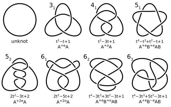
Figure 1.
Prime knots with 6 and fewer crossings. Knot theory notation, Alexander polynomial, and circuit topology string notation are provided for each knot. is called a trefoil. is called a figure-eight knot. , , , are the knots found in proteins [12,13].
In this paper, we will consider chains with different geometrical shapes. In order to make sure that two chains cannot be deformed into each other, we will join their ends to form a mathematical knot and then we calculate the so-called Alexander polynomial. Its definition can be found in any knot theory textbook [10]. There is a rigorous mathematical algorithm for how to calculate it. In our previous paper [11], we demonstrate it step-by-step for the objects most relevant in our approach and discussed in the next section. If two knots have different Alexander polynomials, then these knots must be different. The inverse statement is usually correct, but not always.
An application of knot theory to proteins is centered around a search for prime knots in a spatial protein structure. The only knots that have so far been found in proteins [12] are , , , and . What is a fundamental reason for this choice? What property exactly separates these knots from other knots? The answer to the second question is known. The knots found in proteins can be formed following the so-called twisted hairpin folding mechanism [14] outlined below. This mechanism is rather a phenomenological explanation that does not provide a fundamental difference between knots in terms of knot theory. In principle, a topological theory alone is not able to provide such a reason because physical properties of the chain must matter. In our theory, the twisted hairpin mechanism appears naturally as part of the formalism. A few years ago, the concept of circuit topology was suggested in order to account for intra-chain contacts [15,16,17], which are also very important for proteins. Very recently, circuit topology was generalized to account for chain entanglement as well, focusing on applicability to real-life molecules [11]. The new framework is still in its development stage and lacks certain rigorousness, especially in comparison to very-well developed knot theory. In this study, we attempt to strengthen the foundation of generalized circuit topology and demonstrate that this theory appeals to the “natural and inherent” language describing entanglement. To demonstrate this, we will, among others, re-discover some known results, which appear smoothly as an internal part of circuit topology. We believe it will be useful for molecular engineering and will help puzzle out the design principle of naturally evolved protein knots.
2. S-Contacts
We are looking for basic structural units which would comprise a molecular knot and be invariant to the knot structure, i.e., the “smallest piece of entanglement” that would not change upon a knot deformation. By a deformation, we understand any manipulation with a chain as long as the chain is not broken. One should keep in mind that any chain is an open structure, i.e., it has two ends. By passing ends through knots, we can tie or untie anything. Therefore, the ends must not participate in any manipulations, so that we do not change the topological structure of the chain. Additionally, we recognize the fact that molecules are three-dimensional, hence our formalism is built in 3D, so for the most part, we do not consider projections. On the other hand, it makes it harder to describe the mutual position of different segments of a chain. Unlike in 2D, in 3D there are no crossings of a chain and the corresponding segments of a chain might be distant in space, hence one cannot strictly define a loop. In what follows, these terms should be understood merely as references to certain segments or configurations of a chain in 3D, and as a tribute to the fact that all drawings are inevitably flat, i.e., 2D. A single loop, i.e., one twist of a chain (or a rope) that leads to only one crossing (or no crossings at all in certain projections), is not stable in the sense that it can easily be undone (untied) by stretching the chain, and hence it cannot serve as a structural unit. Indeed, a structural unit cannot disappear: once it is found, it must always be there. To make a loop stable, one should “fix” the loop by threading the chain through it. Figure 2a shows all four possible resulting structures drawn in the way to visually single out the loop and to easily trace how the loop gets fixed. Keep in mind that we are looking for the basic structural units, i.e., we are fixing the loop in the simplest possible way. In principle, the chain can wind around the loop several times before threading the loop, or it can participate in another piece of entanglement. All these effects lead to a creation of several structural units connected in some specific way. This will be considered in the next section.
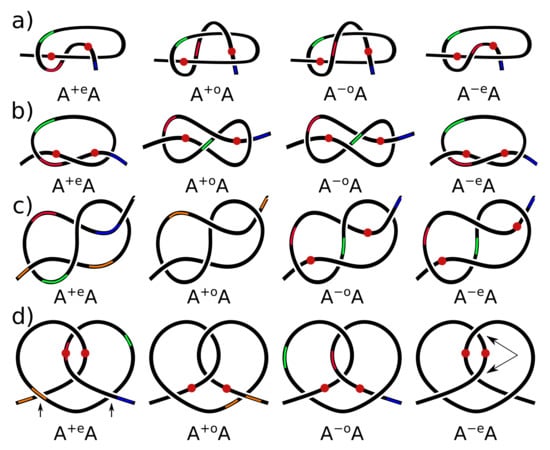
Figure 2.
A list of s-contacts. All the chains in each column are equivalent, i.e., can be deformed into each other. All the chains are 3D structures, not projections. (a) The definition of s-contacts. (b) The “flat” representation of s-contacts. (c,d) Other equivalent representations of s-contacts where the loops are not easy to spot. A change of chirality, i.e., of the sign +/− in the notation, means flipping of all crossings in the representation. Red balls indicate contact sites. Colored stripes are added to make the equivalence of different representations more visual.
Each basic structural unit is called an s-contact, or a soft contact, and cannot by untied by stretching the chain. The term “contact” was coined to stress similarity to intra-chain, non-entanglement contacts, which can also be treated by circuit topology [11], but are not considered in the present paper. Each contact must have two sites. (In case of intra-chain contacts, contact sites are the two chain segments that are linked together). An s-contact is supposed to be contained between its contact sites, i.e., contact sites are the boundaries of the entangled piece of the chain, as viewed while moving along the chain. We define that contact sites are located where the chain passes through the loops, so that the entangled segment is located in-between. What happens to the chain outside to the structural unit (i.e., on either side from the contact sites) is irrelevant. Since s-contacts, and real molecular chains, should be considered as three-dimensional entities, the exact position of contact sites depends on many parameters [11], e.g., on the knot tightness, but it always represents the knot structure. Additionally, contact sites can migrate along the chain during a chain deformation. This uncertainty is essential in order to be able to catch the fixed topological structure of a flexible, mobile chain. If the chain were solid, incapable of any movements, or in case of a static chain projection, s-contact sites would not be movable. Contact sites are depicted with a red ball on several structures shown in Figure 2.
Figure 2 shows several equivalent representations of s-contacts. Each column represents only one structure, i.e., all four structures in each column can be deformed one into another. It might not be immediately obvious, therefore we put colored strips to ease the tracking of corresponded deformations. Let us consider the first column in Figure 2. Panel “a” is designed to highlight the loop being fixed by the chain end passing through it. If we move the chain segment at the top to the left to make it more symmetric, we will end up with panel “b”. If we move the red and blue strips from panel “a” up, we will get panel “c”. Therefore, even though the structures within one column are perceived by an eye as different, a 3D transition between them requires just a minor deformation. Such deformations are irrelevant and occur all the time in real molecules. In our theory, we do not want to notice these minor deformations because they do not make any physics contribution. We do not want to be concerned with them because they do not change the properties of the molecule. This is why we use such a flexible definition of s-contacts and s-contacts’ site, i.e., we make them sensitive to the molecule’s structure, which cannot be changed, but ignorant of all irrelevant details that in real molecules are nothing but noise. While threading the loop, we have to go around one segment of the chain, thereby creating another loop. Therefore, each of the four structures is symmetric: each consists of two identical loops hooked together. Following the chain in either direction, left-to-right or right-to-left, we see the same structure, which is most noticeable in panel “c”. The representation in panel “d” shows that each s-contacts consists of two loops. This representation is topologically identical to the other representations, but is more distinct from them. A transition to it requires a major deformation. This representation can for convenience be considered flat as a limiting case of 3D, which will be useful in the next sections. This “flat” representation resembles projections used by knot theory and can be useful in building a link between knot theory and circuit topology.
Contacts should be given names. We usually use capital letters, such as contact A, contact B, etc. In Figure 2, each chain has one contact. If we move along the chain from any end and write down contact sites we encounter, we will get AA, which is a code for one contact. How to distinguish between the four different s-contact shown in the figure? Figure 2d shows the same s-contact from Figure 2a in a different representation where loops are easier to spot. The both representations are topologically equivalent and one can continuously transition from one to another without breaking the chain. Each s-contact is a connection of 2 loops, which are easy to recognize in Figure 2d. Each connection has 4 crossings, which can naturally be split into 2 independent pairs: the crossings forming the loops (located on the sides) and the crossings forming the connection between the loops (located in the middle). The crossings in each pair are not independent. If one of them is flipped, the s-contact unties, as should be clear from the illustration. Each independent crossing can take two values, depending on which chain segment is on top. Two values of two independent crossings give rise to 4 different structures. It means that there are only 4 s-contacts possible, and hence our set of s-contacts is complete. The pair of crossings defining the s-contact chirality (i.e., forming the loops) is depicted on the left-most s-contact. The chirality of each loop is defined by the conventional right-hand rule. If the loops have different chirality, then none of these loops have been fixed by threading the chain through them, which means this structure will untie. In other words, despite consisting of two loops, s-contacts can only be either positive, AA, or negative, AA.
The other independent pair of crossings, shown on the right-most s-contact in Figure 2d, defines how the two loops are hooked together. If the chain passes through the loop in the same direction as the chain shifts in each loop at the crossings defining chirality, such an s-contact is called “even”, AeA. If the chain passes through the loop in the opposite direction, the s-contact is called “odd”, AoA. Hence, the only 4 possible s-contacts are AA, AA, AA, and AA. This notation is called the string notation of circuit topology. It codes a chain entanglement as a string of letters. One of the advantages of this notation is the ability to apply combinatorial analysis directly to a description of entanglement. Additionally, note that the attributes introduced above are universal and do not depend on the chain orientation, i.e., in which direction we move along the chain, left-to-right or right-to-left.
Let us consider s-contacts in the view of knot theory. To form a knot from a rope, one has to join its ends. To make a rope form a knot, one has to cut the knot somewhere. AeA corresponds to . This knot can be right-handed, as in Figure 1, or left-handed if all the crossings are flipped. AoA corresponds to , see Figure 3a for a visualization of the sequence of corresponding deformations. This knot is known to be achiral (amphichiral), i.e., , i.e., AA and AA can be deformed into each other. The sequence of corresponding moves is shown in Figure 3b. However, both AA and AA should be kept and considered as separate s-contacts because, as will be shown below, they comprise different knots in a presence of other s-contacts. Can we distinguish AA and AA when they are along? Topologically speaking, we cannot, and knot theory is clear about this. Geometrically speaking, it boils down to the notion of stability, similar to retaining or quenching slip-knots. Namely, the deformation needed for a transition between AA and AA costs energy. If the cost is low, the transition can occur spontaneously. Otherwise, it will not occur, rendering the molecular knot stable. We will discuss it in Section 4.2. However, note in Figure 2b that AA and AA look like a mirror reflection. Such a flip of symmetry matters in proteins, so we must retain it for molecular engineering purposes.
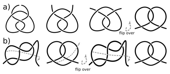
Figure 3.
Properties of s-contact AoA. (a) AoA corresponds to knot (see Figure 1). (b) Transition between AA and AA, demonstrating that AA=AA ≡ AoA.
So far, we identified 4 stable “basic structural units” of chain entanglement, and called them s-contacts. Note that if we flip only one crossing in any chain from Figure 2, the s-contact will disappear and that chain will untie. Any messy blob of a rope is held together by loops hooking to each other, which is the essence of entanglement and the definition of s-contacts. In the next section, we will consider how s-contacts can be connected to each other. S-contacts might not be easy to spot in illustrations, even in such a simple case of knot. Where exactly are s-contacts in the prime knots shown in Figure 1? We will break it down below, but at the current state of our theory, it is easier to go in the opposite direction, i.e., to tie s-contacts on a rope and then identify the resulting knot. In the present paper, we tie s-contacts, we tie knots and we want to see how it works. Here, we focus on developing the formalism of s-contacts. When it comes to analyzing real folded molecules, the procedure is the opposite: we have to identify s-contacts based on the input from experimental data, for example based on the positions of all atoms in the molecule. This is a separate problem, which should be treated numerically and will be consider in another paper. So far, a protocol, along with a computer code, has been developed to treat intra-chain contacts [18].
3. SPX Configurations of S-Contacts
One s-contact has two contact sites and appears in the string notation as AA where each letter signifies this contact’s sites. Two s-contacts, AA and BB, can occur in three different configurations defined by permutations of two pairs of letters: AABB, ABBA, and ABAB. Because s-contacts can have any name, the configurations ABAB and BABA are identical. These three configurations are called series (S), parallel (P), and cross (X), and comprise the SPX relations. Regardless how many s-contacts a knot consists of, these pair-wise relations always hold and are shown unambiguously by the string notation. For example, in AACDCBDB, all relations are immediately obvious, e.g., the contacts A and B are in series, and contacts C and D are in cross, etc. Therefore, a consideration of all pairs of s-contacts is sufficient to describe a chain entanglement. Indeed, the string notation lists all contact sites as they appear along the chain and can be unambiguously deduced from the relative positions of all pairs of contact; thereby it completely specifies (or codes) the chain entanglement in terms of s-contacts.
Series and parallel configurations are easy to visualize. Figure 4a shows two s-contacts in series; Figure 4b shows two other s-contacts in parallel; and contact sites are marked with colored balls. Note that in Figure 4b the internal contact, marked with blue balls, can be placed in different loops of the external contact marked with red balls. However, blue balls will always be between red balls, i.e., the contacts are always in parallel with the same string notation (ABBA). Here, we do not specify the symmetry and chirality because this rationale works for any kind of s-contact. SP configurations with other types of s-contacts can be drawn in a similar manner. Note that chains from Figure 4a,b look very different not only because they consist of different s-contacts, but also because of the different relations between s-contacts, i.e., series and parallel. However, the relations of s-contacts can be swapped between each other by a sequence of moves shown in Figure 4c. Notice that contact B is not altered in any way during the deformation. Hence, it can be replaced by any other kind of s-contact or any arrangement of s-contacts. Contact A throws out a loop and gets deformed. A similar deformation can be applied to any kind of s-contact. Applying this deformation to one s-contact after another, one can push s-contacts inside other s-contacts or pull them outside, thereby dragging an s-contact along the string in string notation. For example, one can turn AeA BB CeC into AeA CeC BB (i.e., to ). In general, because a pair-wise consideration is sufficient, any set of s-contacts consisted of only SP configurations can have any fraction of S and P relations as long as their total number is constant. As limiting cases, such a set can be deformed into all s-contacts in series or all s-contacts in parallel. Because in this case s-contact can be singled out, AA and AA are indistinguishable in case of series and parallel configurations (since they correspond to knot which is achiral). However, AA and AA cannot be deformed into other s-contacts (since knot is not achiral). Two entangled chains consisted only of SP configurations can be deformed into each other only if they contain the same number of s-contacts of each kind. For example, the chains in SP configurations from Figure 4a,b contain different kinds of s-contacts, and therefore cannot be deformed into each other.
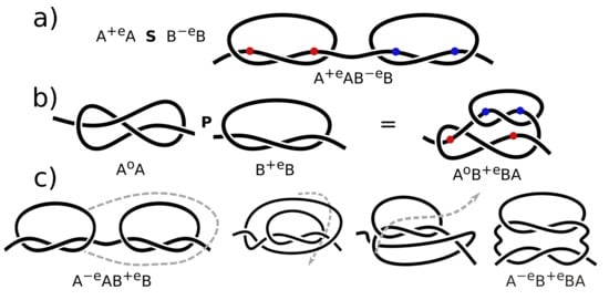
Figure 4.
SP relations. (a) Two s-contacts in series. (b) Two s-contacts in parallel. (c) A transition between series and parallel configurations. The dash lines show the sequence of movements to turn the series configuration into the parallel configuration.
The transition from Figure 4c is important in the context of protein folding and has been studied in the literature [19]. Knot theory cannot distinguish these two configurations because they correspond to the same knot [11]. However, in real molecules, such a transition between these configurations requires energy and once again comes down to the question of stability; the transition might be very probable or might never happen, depending on the physical properties of the chain. Circuit topology aims at addressing this question and provides consideration of different levels of structural stability.
SP configurations are similar to the notion of a connected sum used in knot theory. To form a connected sum of two knots, one should cut each knot and merge the resulting ends together, which is the procedure demonstrated in Figure 4. Consequently, based on the connected sum properties, the Alexander polynomial of several s-contacts in series or in parallel is a product of Alexander polynomials of each s-contact.
Cross (X) configurations are very different from SP configurations. Each s-contact consists of two loops. Figure 5 shows all possible arrangements of two pairs of loops. Indeed, the loops in this “flat” representation can be counted similarly to counting s-contact sites: the loops can be in series, in parallel, and in cross. The S operation is obtained by joining the red and blue s-contacts together at one endpoint of each. The connection between the two contacts is shown in black. The P operation is obtained by cutting open the bottom arc of the red s-contact and joining the endpoints of the blue s-contact to the endpoints of the cut open part of the red s-contact. The X operation requires altering the s-contact sites (and hence, the loops) as in ABAB. It is obtained by first cutting open the bottom arc of both the red and the blue s-contacts to obtain red arcs and and blue arcs and , and turning the pictures so that and are above and , respectively. Next, one endpoint of is attached to one endpoint of and the other endpoint of is attached to one endpoint of , and one endpoint of is attached to an endpoint of . This gives us a single arc, alternating between red and blue, which has one endpoint on and the other endpoint on . The case when one loop is shared by a pair, i.e., C configuration, is considered in the next section. This “flat” representation is convenient for listing and counting cases because it retains the number of loops, but one should keep in mind that these flat structures can always be deformed into 3D. In S and P configurations, the loops belonging to the same s-contacts are hooked together. Each pair of loops can be separated and cut off the whole chain. It is not possible to do in X configuration where loops belonging to different s-contacts are connected. Contacts AA and AA are identical, i.e., can be deformed into each other, only as long as their loops are free to move as is the case in SP configurations, see Figure 3. In X configuration, loops from one s-contact are connected to loops from another s-contact, and hence are not free. Therefore, contacts AA and AA are not identical and lead to different knots when they are parts of X configuration.

Figure 5.
SPX and concerted (C) configurations of two s-contacts in the loop representation. S-contact sites are shown in X configuration. Here, not complete s-contacts, but only the loops are color-coded. Recall that s-contact sites indicate the “borders” of the s-contact, i.e., the borders of the corresponding piece of entanglement; however, different s-contacts can share the same segment of the chain.
Let us consider the transition between S and P configurations by looking at the illustrations in Figure 5 and see again that it does not work for X configuration (C configuration will be considered in the next section). Additionally, the single deformation shown in Figure 4c is obvious only in case of two s-contacts. What if there are more s-contacts? What is the general rule? Topologically, we can stretch the chain but we should not break it. When two loops are joined into an s-contact, they are connected and cannot be separated. In contrast to loops, one single s-contact can be moved along the chain freely. So, we take the blue contact from the right top corner of Figure 5 and move it to the left. It passes through the left loop of the red contact and then moves down to the bottom of the red contact. By this manipulation, we turned S configuration into P. In other words, we are only allowed to move the whole contact along the chain, but not contact sites. The transition AABB ⟶ ABBA should be understood as the whole contact B moves to the left, but not as one contact site of contact A moves to the right. Following the same logic, let us add contact C to the left of X configuration in Figure 5. The resulting string is CC ABAB. Contact C as one entity can move through the loop of contact A to form A CC BAB or further to ABCCAB; but it can never lead to CACBAB or ACBCAB. As a consequence, X configuration cannot be turned into SP. Here, the crossings in Figure 5 make no difference in the rationale, hence this conclusion is applicable to any kind of s-contacts.
There are 4 s-contacts (AA, AA, AA, AA), which gives rise to configurations of 2 s-contact in cross, which can be written as a 4 × 4 table. This table is symmetric owing to the left-right symmetry, i.e., which direction we move along the rope, e.g., ABAB vs. BABA. This leaves 4 configurations on the diagonal and 6 configurations above (or below) the diagonal, i.e., 4 + 6 = 10 configurations. As shown in Figure 2, a change of chirality in a single s-contact, i.e., a change of all signs in the string notation, leads to a flipping of all crossings. This property holds for any combination of s-contacts. Indeed, flipping all crossings means a mirror reflection of the whole knot. Due to this symmetry, the number of configurations to consider can be further reduced. On the diagonal, ABAB and ABAB can be treated (or drawn) as one configuration. Similarly, ABAB and ABAB. The same holds for two non-diagonal configurations: ABAB vs. ABAB and ABAB vs. ABAB. It leaves us with 10 − 4 = 6 configurations which are shown in Figure 6. Let us count these 6 configurations again, but this time geometrically. First, we tie contact A whose contact sites are marked with red balls. We made one of the loops corresponding to contact A the largest in the illustration in order to make it easier to spot contact A. This loop can always be shrunk without changing the overall topology. After contact A is “fixed”, i.e., after the second red ball, where can the rope go? It can go away, which would create SP configurations. Or the rope can pass through this large loop again, thereby creating another s-contact in cross with contact A. Figure 6 shows all possible route of the rope leading to another s-contact. If the rope keeps passing though the large loop, it will just create more and more s-contacts. If the rope keeps winding around the large loop, it will lead to the relation considered in the next section. Note that ABAB and ABAB look very different and their Alexander polynomials are different, though the only difference between them is the chirality of contact B. It is a rigorous proof that even though BB and BB are identical while standing along, i.e., while being in series or in parallel to other s-contacts, in cross configurations they lead to different composite structures. Hence, all 4 s-contacts should be retained.
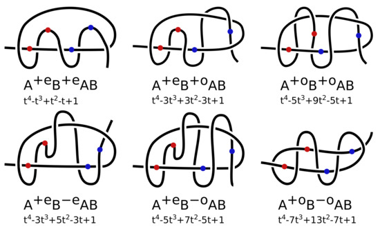
Figure 6.
All independent (up to symmetry) configurations of two s-contacts in cross. The flat notation from Figure 5 is accompanied by an illustration of possible paths in tying the second s-contact. Contact sites are shown as colored balls. String notation and Alexander polynomials are provided.
In order to easily verify and visualize the correctness of strings provided in Figure 6, one can either calculate the Alexander polynomial or untie one of the s-contacts. For example, in ABAB one can unhook the left site of contact A (red balls), so that contact A disappears and only BB is left. In the drawing, this procedure means that the left-most crossing is flipped, so that the left red ball no longer passes through the loop. Then, the rope can be deformed into the configuration from Figure 2a by reducing the loop freed by the flipping. The same holds for the right site of contact B (blue balls). Additionally, consider ABAB. After the second red ball, the rope wraps around the large loop and gets “fixed” by passing through the large loop at the location of the second blue ball. If the rope does not pass through the large loop, so there is no blue ball, then no matter how many times the rope wraps around the large loop, the second contact will not be formed. Indeed, this “spiral” around the large loop will not be stable and will be easily untied by pulling the rope ends apart.
Each of the four s-contacts has an Alexander polynomial degree 2. Two s-contacts of any kind in any of SPX configurations have Alexander polynomial degree 4 (these polynomials are provided in the corresponding figures). n s-contacts of any kind in any SP configuration have Alexander polynomial degree . Indeed, SP configurations correspond to a connected sum in knot theory, which proves that the Alexander polynomial of the sum equals a product of the Alexander polynomials of single connected knots [10], in our case s-contacts. It is reasonable to expect that the Alexander polynomial degree scales the same for X configurations as well. Indeed, Figure 6 shows a clear pattern of Alexander polynomials, depending on the kind of s-contacts in cross. The easiest pattern appears for positive even s-contacts. The Alexander polynomial of AA is ; ABAB corresponds to , see Figure 6. One can predict that ABCABC has the Alexander polynomial . The corresponding prime knot, , is not drawn here, but can be easily deduced from the pattern, and it indeed has this Alexander polynomial. Let us formulate a recipe for how to construct knot. AA is shown in Figure 2a. Then, the right end of the chain makes one circle around the horizontal segment and forms ABAB from Figure 6. Another similar circle around the horizontal segment will lead to ABCABC. It would be interesting to investigate further on the relationship between Alexander polynomials and s-contacts, but it is beyond the scope of the present paper. Here, we only hypothesize that such a relation exists. One should, however, note that the chains in Figure 6 have a different number of crossings, correspond to prime knots, which also have another number of crossings; yet they all have Alexander polynomials of the same degree. We attribute it to the pattern we outlined.
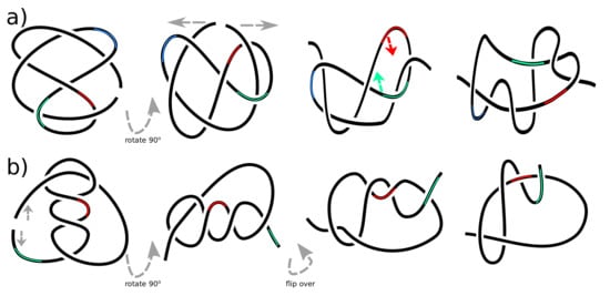
The cross configuration of chains in different forms in Figure 6 look nothing alike, yet they are topologically identical. One can verify it by calculating Alexander polynomials provided in Figure 6. To change to another chain in the “flat” representation of Figure 5c, one has to flip just a few crossings (consult Figure 2d). Therefore, all the different-looking chains from Figure 6 look extremely similar when presented as loops. What about a 3D shape of real molecules? It depends on the physical and chemical properties of the molecule. If these properties require a minimization of the bending energy of the chain, the 3D shape would resemble a distorted version of the “non-flat” chains in Figure 6. The “flat” representation is just convenient for theoretical studies, visualization of the formalism and tying simple knots. Despite having the same Alexander polynomials, the configurations from Figure 6 do not visually resemble the prime knots from Figure 1. One can deform them one into another. However, such manipulations require many-step, major deformations that are hard to follow and, quite frankly, tedious to draw. More importantly, this would have no practical use. Indeed, we aim at describing proteins and other linear macromolecules. In principle, the 4 s-contacts (, , , ) are supposed to be found and identified automatically by a computer, not by a naked eye. Yet, it does look suspicious that s-contacts are not obvious in prime knots. Figure 7a shows the equivalence of knot from Figure 1 and ABAB form Figure 6. Surprisingly, it requires only a minor deformation. and can be treated similarly. and will be discussed in the next section.
4. Concerted Contacts
Concerted contacts first appeared in the context of intra-chain contacts, which are not due to entanglement. Unlike s-contacts, intra-chain contacts have specific locations of their contact sites. What happens when two intra-chain contact sites are too close to each other so that they cannot be distinguished, as often the case in experiments? Such contact sites are placed inside parentheses and are possible in two variants: concerted series A(AB)B, which resembles A(BA)B, and concerted parallel (AB)BA, which resembles (BA)BA. When it comes to entanglement, contact sites of s-contacts are not specific and can move along the chain. However, some form of concerted structures still appears.
4.1. C Configuration
Each s-contact consists of two loops. In the “flat” representation used in Figure 5, two s-contacts cannot have more than 4 loops. The case when two s-contacts have 4 loops is considered in the previous section. In the current section, we will consider two s-contacts having three loops, where the middle loop is associated with both s-contacts. This ambiguity in number of loops arises from the fact that loops are not invariant of entanglement, while s-contacts are invariant.
Let us consider two s-contacts and count how many configurations with a shared loop they can have. Each s-contact consists of two loops. The loops of each s-contact must have the same chirality, otherwise it would not be an s-contact because the structure will untie. With three loops it is problematic because the loop in the middle is shared by the s-contacts. Three loops give rise to configurations. Two of them, where all the loops have the same chirality, i.e., and , are identical to two s-contacts in cross, namely ABAB and ABAB. It is expectable because in these configurations there is no chirality conflict between the s-contacts via the shared loop. The other 6 configurations are , , , , , . Note that the first pair and the second pair possess the left/right symmetry, hence one from each pair can be omitted. Among , , , , two pairs are symmetric with respect to chirality (), which leads to flipping all crossings. Therefore, we have only two configurations left to consider, and . Each of them leads to 4 cases, depending on how the two pairs of loops are hooked to each other. either unties or coincides with AA or AA. In other words, it leads to already known s-contacts. Thus, we counted all the configurations consisted of 3 loops and the only configuration which is left, , leads to a new kind of relations of s-contacts.
The last remaining configuration, , leads to (AB)AB and (AB)AB. Its symmetric leads to (AB)AB and (AB)AB, shown in Figure 8. In these configurations, contacts A and B share a contact site and will both untie simultaneously if this loop is unhooked. This property distinguishes them from SPX configurations where two contacts cannot be untied with one move. In terms of Figure 5, they share a loop and will untie if the loop is undone. As stated in the previous section, a transition between the “flat” representation in Figure 5 and the representation in Figure 8 typically requires major deformations and is hard to follow. However, one can see some resemblance. Let us consider the first line in Figure 8. Contact A in AA has two loops. Then, the right end of the chain goes around and forms contact B, which shares one loop with contact A (where red and blue balls coincide). So, two loops from contact A plus two loops from contact B, accounting for one shared loop gives 2 + 2 − 1 = 3 loops. The left-most loop is shared and, if untied by flipping the left-most crossing, both s-contacts disappear. The right-most loop belongs to and unties only contact B. The middle loop, which belongs only to contact A, cannot be untied all along since it is in the middle. Hence, one cannot untie only contact A, which can be seen from the illustration as well. When contact C is formed, there are 4 loops and the left-most loop is shared by all the s-contacts. Based on the analogy with intra-chain (i.e., non-entanglement) contacts considered in our earlier work [11], if contacts share contact sites, they are called concerted. The corresponding relation is called the C configuration, and is written as a cross configuration, i.e., (AB)AB, not (BA)AB. In addition, note that ABAB and (AB)AB are two different configurations, X and C, correspondingly. Though we do not consider intra-chain contacts in this paper, we will briefly mention a minor difference in the terminology for intra-chain contacts and s-contacts. While concerted s-contacts are written in cross with parentheses, concerted relations of intra-chain contacts are written in series or in parallel. It is motivated by the resemblance of properties of these relations. To some extent, C configuration of s-contacts might seem as a specific case of X, and some of their properties are indeed similar, but not identical. For example, both C and X cannot be turned into another configuration (unlike P and S).
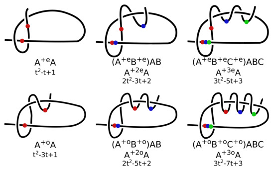
Figure 8.
Concerted s-contacts shown in the flat notation of Figure 5 and in the notation where one loop is highlighted of Figure 2a. The later notation illustrates the twists needed to form these knots. Contact sites are depicted with colored balls. String notation and Alexander polynomials are provided.
As clear from Figure 8, C configuration is possible only for the same kind of s-contacts, e.g., (AB)AB is impossible. Indeed, after passing through the large loop and forming contact AA, the chain should pass the same large loop in the opposite direction in order to form a contact with a different chirality, i.e., contact BB. However, it forms a slip-knot, which is not an s-contact and will be considered in the next sub-section. Hence, the notation can be simplified: (AB)AB → AA, where the digit signifies the number of s-contacts. Note that C configuration is not symmetric. If the rope is read from another end, the full string notation should be used, e.g., AB(AB). This simplified notation is used in Figure 1 because, unlike chains, mathematical knots are closed structures and need to be cut to become chains. No matter where a prime knot is cut, the resulting linear chain is always the same. Using a simplified notation is desirable because it stresses that concerted s-contacts are, to some extent, only one contact because it can be untied by one move unhooking only one loop. Alexander polynomials of single s-contacts and concerted s-contacts, Figure 8, all are degree two. The factor at shows the number of s-contacts in the concerted contact, e.g., , which is AA, consists of 3 s-contacts. This is in line with the conjecture made in the previous section arguing that the Alexander polynomial degree scales with the number of s-contacts for all SP, X and C configurations. Indeed, SP is similar to a connected sum and the corresponding scaling of Alexander polynomial is well-known in knot theory. C corresponds to a special class of knots called twist knots, for which the scaling was proved as well. X, as far as we know, does not have a direct counterpart in knot theory, and so the scaling conjunction for X has not been proven (or even considered) yet.
When we had just introduced s-contacts in Section 2, we said that many wraps around one of the loops lead to several s-contacts. This is shown in the right-most column in Figure 8. Notice that if we undo the concerted contact site which fixes the loop (right blue ball), then the whole thing will untie. However, if we undo the left blue ball, only one s-contact will untie and the other will stay. The difference between the right-most column and the other columns is that we move along the chain in different directions, while concerted configurations do not possess this symmetry. The string notation represents it clearly because the parentheses are located on different sides on the strings. Note that both (AB)AB and AB(AB) have the same simplified notation, AA, because they correspond to the same prime knot.
Concerted contacts are closely related to each other. If we twist a rope once, we form a loop. By threading the rope through this loop, we get AeA. If we twist a rope twice and thread it, we get AoA, see Figure 8. If we twist a rope three times and thread it, we get AA. Twisting four times gives AA, etc. This is the twisted hairpin mechanism [12,14], which leads to a formation of twist knots. All the knots found in proteins can be tied by this mechanism. In other words, concerted and only concerted contacts have been found in proteins. Here, we would like to point out that C configuration does not arise as a result of some artificial mechanism of twisting the rope, but it comes out from the bottom-up consideration of possible arrangements of contact sites of s-contacts, which is more fundamental and general. The swirling part of concerted knots can be seen in Figure 1, especially for . However, their s-contacts are still not so easy to spot. Figure 7b demonstrates the series of deformations needed to transition from Figure 1 to Figure 8 for . can be treated similarly. The location of the cut is irrelevant. The cuts in Figure 7 are chosen so that the smallest deformation is required.
4.2. Slip-Knots
As we stated above, (AB)AB is impossible. What if we try to tie it anyway? After all, we are interested in considering all possible configurations. Figure 9 shows the treatment of even contacts, i.e., AeA. Odd contacts, i.e., AoA, can be treated similarly. In order to form a negative contact along with a positive contact, one has to reverse the direction of the chain. In Figure 9, it is marked with a green ball, which is located where the chain passes through the s-contact. The left part of the rope up to the green ball is the same in all configurations. Let us consider it. Contact A (red balls) consists of two loops. The second red ball shows where the rope passes through the large loop, closing (or “fixing”) contact A. Then, the rope passes through the large loop again (green ball), so potentially it might be a sign of another s-contact. However, in this case no s-contact is formed because it does not match any structure from Figure 2. In fact, we end up with the structure similar to the first or the last ones in Figure 2a, but with the middle crossing flipped. So, we have an event worth noticing (passing through the large loop), but there is no s-contact. In the string notation, this event is shown as a subscript, where the sign indicates the direction in which the rope passes the s-contact: “+” if it coincides with the positive direction of the s-contact, “−” otherwise. Such a subscript forms a loop, but this loop is not fixed, so it does not form an s-contact. To some extent, subscripts can be viewed as a half of an s-contact. In other words, if the rope passes through a loop and fixes it, it creates an s-contact; otherwise it is unknot. If the rope passes through an s-contact and fixes it, it creates another s-contact; otherwise it creates a subscript. Subscripts appear only when the rope passes through an s-contact. For example, in Figure 6, the rope passes through various loops, especially in configurations with different symmetries of contacts. However, it does not create subscripts because those loops are not s-contacts.
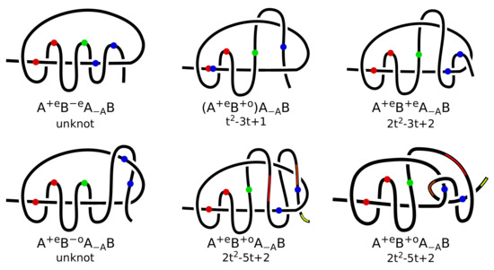
Figure 9.
Configurations with subscripts. Contact sites are shown as red (contact A) and blue (contact B) balls. The subscript is shown as a green ball. String notation and Alexander polynomials are provided. If the rope is followed from left to right, then the positive direction of contact A is up, towards the reader.
S-contacts are stable, i.e., cannot disappear or be untied, while subscripts are not stable. In any configuration shown in Figure 9, the rope segment between the second red and green balls forms a slip-knot, which can be untied by pushing it back through contact A (red balls), which would eliminate contact A and the corresponding subscript. In terms of knot theory, this transition is a sequence of Reidemeister moves. Hence, knot theory does not see subscripts and slip-knots. Why does circuit topology ignore unstable loops, but consider unstable subscripts? It is because one has to find a balance between unstable and irrelevant. Loops are very flexible structures, which can appear and disappear easily. Subscripts, even though they can disappear, are more stable than loops and are observed in proteins as slip-knots. Whether a subscript is “metastable” or not, depends on the physical properties of the rope and the size of the corresponding s-contact. A related issue in the context of stability is that, while forming a subscript, we do not specify where exactly the s-contact is pierced by the rope. To some extent, here the s-contact is considered as a loop, not as two loops. So far, we deem it as sufficient because here the s-contact works only as a restriction of motion of the rope. What part of the s-contact exactly restricts the motion is less relevant.
Figure 9 shows two equivalent representations of the same rope configuration, ABAB, i.e., they can be deformed into each other. The deformation is outlined in the figure by colored stripes and should be performed in 3D because these illustrations are not projections, but 3D structures. Let us consider contact B (blue balls) in both of them. In the chain on the left, contact B resembles that s-contact in ABAB from Figure 6. In the chain on the right, contact B resembles that AA from Figure 2b. Note that the both chains are visually different, but have the same Alexander polynomial, same string notation, correspond to the same knot, and can be deformed into each other. In terms of circuit topology, these two chains are equivalent. If these chains were an actual molecule, which configuration would the molecule attain? We do not know because it depends on the physical properties of the molecule.
The first column in Figure 9 shows the rope going downwards after the subscript, i.e., after the green ball. In these configurations the chirality of the s-contacts are different and they are unknot, i.e., will untie if the chain ends are pulled. The other configurations show the rope going upwards, which leads to the same chirality of s-contacts. These configurations cannot be untied. Therefore, consider the chirality pattern in circuit topology. If two loops have different chirality, they are unknot. If two loops have the same chirality, they form a stable s-contact. One level up: two s-contacts with the same chirality can form a stable concerted contact; while two s-contact with different chirality can form a slip-knot, which can be untied. Untied configurations with subscripts with the same chirality of s-contacts lead to concerted configurations, which must have the same chirality. The symmetry between concerted configurations and configurations with subscripts goes further. In this paper, we first derived all possible s-contacts and then considered all possible stable configurations of them. In Figure 8, we found that some combinations of s-contacts are impossible to be concerted. However, in Figure 9, we see that these impossible configurations can be described by subscripts. So, concerted configurations and configurations with subscripts are complimentary to each other. Subscripts are not stable as s-contacts, but also not completely unstable as loops. S-contacts consist of 2 loops, while subscripts consist of 1 loop. Hence, we view subscripts as a half of an s-contact. Laying out the formalism, we try to build an analogy between intra-chain (non-entanglement) contacts and s-contacts that describe entanglement. Since a subscript is similar to a half of s-contact, contact A (red ball) and the subscript (green ball) can be vaguely considered as being in series and sharing a contact site via the slip-knot. Hence, configurations with subscripts are analogous to concerted series configurations of intra-chain contacts. In other words, we found that entanglement and intra-chain contacts have the same set of configurations in term of circuit topology, namely series, parallel, cross configurations for both intra-chain contacts and s-contacts, concerted parallel for intra-chain contacts vs. concerted s-contacts, and concerted series for intra-chain contacts vs. subscript configurations for s-contacts. This analogy matters for a completeness of circuit topology description of entanglement.
As proclaimed above, we want circuit topology to be able to describe molecular operations easily and intuitively. It can be achieved by means of string notation. Let us consider (AB)AB from Figure 9 because it has both kinds of concerted contacts. Let us cut it at the loop of the slip-knot, i.e., between red and green balls. In string notation it looks like (AB)A ∣ B. The letter B in the left part occurs only once, so it cannot be fixed, hence it disappears. The left part turns into AA, as expected because this slip-knot is based on a trefoil. The right part, B, has no pairs of letters, so it is an unknot. One can also see how the two parts are intertwined, since one part can be trapped inside of another part. The number of such connections equals the number of broken contacts in cross plus the number of subscripts. In our case, there are no contacts in cross and there is only one subscript. Hence, the right part of the original chain passes once through contact A of the left part. Let us do the same manipulation with ABAB from Figure 9. We get ABA ∣ B. The left part is a trefoil; the right part is an unknot. Due to the subscript and broken contact B, the right part passes twice througt the left part. The left part passes only once through the right part (due to contact B). One should be careful with this last statement because the right part has no s-contacts, so one cannot strictly pass though it. However, the right part swirls around the left part, forming a kind of a tunnel, which the left part passes through. It can be visualized in Figure 9.
5. Circuits
We found in Section 3 that contacts as a whole can be dragged along the string, which explains the transition between S and P. What would happen if other relations were present? Let us consider ACABCB. Contacts A and B are in series, but they can never become in parallel because they cannot be dragged along the string. The dragging is blocked by contact C, which is in cross with contacts A and B. Indeed, if we want to drag contact A, we would also have to drag everything locked between the letters “A”, i.e., the letter “C”. However, it is not the whole contact, hence such a drag is forbidden. In our previous work [11], we introduced the notion of circuits. A circuit is a segment of a string, which consists only of pairs of letters and subscripts of the same letters. In other words, a circuit can be isolated from other contacts. By “isolated”, we mean “can be put in series”. Circuits can be dragged along the string. Obviously, circuits can consist of several circuits, e.g., AABCBC consists of AA and BCBC. The number of possible prime knots for a given number of crossings is still unknown [20,21] and our theory might help find it. It would be interesting to further investigate this algebra of s-contacts and the detailed construction of prime knots out of circuits. For example, we said that SP looks similar to a connected sum. Why? It is because the circuit AABB consists of smaller circuits, namely AA and BB, and hence AABB is not a prime knot, which implies that it must be a connected sum of prime knots. In principle, coding entanglement as a string of letters offers an advantage of being able to apply combinatorial analysis (even before considering the algebra of circuit topology operations). In this paper, we employed it in a very mild proportion in order to count the number and kind of possible s-contacts (AA, AA, AA, AA), see Figure 2, and all possible configurations of pairs of s-contacts, Figure 5. Indeed, two s-contacts cannot have more then 2 + 2 = 4 loops, and we considered all configurations consisted of 2, 3, and 4 loops. This pair-wise consideration is sufficient to code entanglement, i.e., to specify the unique string corresponding to the chain, but, as we just saw by ACABCB, the dynamics of the chain, i.e., the mobility of s-contacts, can be affected by other contacts, so that larger scale structures such as circuits have to be considered.
In this paper, we demonstrated how circuit topology can be used to describe simple knots consisted of just a few s-contacts. However, how many are “just a few” in practice? This chain we considered, ACABCB, if s-contacts are assigned symmetry and chirality, leads to configurations. Half of these configurations are chirality symmetric (i.e., all crossings flipped; left-hand/right-hand symmetry). Additionally, configurations are left-right symmetric (i.e., the kinds of s-contacts A and B coincide). Half of these configurations are chirality symmetric as well and we do not want to count them twice. Therefore, independent configuration of the string ACABCB are possible. How many prime knots can we get from here? To turn a chain into a knot, one has to join its ends. In reverse, depending on where we cut the prime knot, we will end up with different-looking chains, which can be deformed into each other. In our example, ACABCB, the left letter “A” and the right letter “B” should be connected to form a knot. Then, we cut the resulting ring of letters at different spots, which gives rise to several strings (chains): ACABCB, BACABC, and CBACAB. The strings are the same up to a cyclic permutation. These chains look different, but they correspond to the same prime knot and can be deformed one into another. Because there are only three such permutations, there are different prime knots described by the chain ACABCB. Analyzing these cyclic permutations by combinatorics, we can easily see which chains can be deformed one into another. There are other strings, apart from ACABCB, made of three s-contacts. The number of different configurations grows fast with the number of s-contacts. Hence, all practically manageable chains involving reasonably complex prime knots are made of three or maximum four s-contacts (and subscripts). We believe it can be useful for engineering new molecular chains, which can be compiled from a small set of these basic structural units.
All the illustrations shown so far came from the pursuit to consider all possible configurations consisting of one and two s-contacts. It is a bottom-up approach when we combine the “basic units” and see which knots we end up with. Let us now go in the opposite direction. We will consider a fairly complicated knot and break it down to s-contacts. As mentioned above, it is a tedious procedure, which should be done by a computer, not by a naked eye. On the other hand, it helps to visualize and appreciate how s-contacts work in real life. We chose to consider knot because it has the same Alexander polynomial as knot from Figure 1. In this paper, we use Alexander polynomials only to distinguish between knots while developing our approach. Alexander polynomials work very well, but fail in some rare cases. Let us see if our circuit topology can catch the different between and . Figure 10a shows a sequence of moves to deform to a more eye-friendly representation with one large loop. All the moves are in 3D. The string notation is (AC)BABC. Note that it is a circuit. Figure 10b color-codes the s-contacts. Every rope segment trapped by a loop restricting its motion, gives rise to an s-contact site or to a subscript. Notice the use of the simplified notation for C configuration and the treatment of the subscripts originated from the loop passing through contact B (marked in dash). So, circuit topology clearly differentiates between and . Note that contains the same s-contact, AA, which comprises . In addition, note that and contain a different number of s-contacts, hence the scaling of Alexander polynomial with the number of s-contacts does not hold in this case. The main reason for this is the presence of subscripts that are not a part of knot theory (see Figure 9 where the pattern is broken as well). Whether chains with mixed operations (SP and X and C) follow the same scaling is unclear.
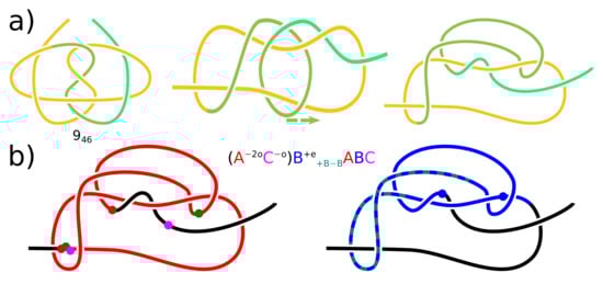
Figure 10.
Knot . (a) A 3D deformation of the knot. Segments are colored to simplify the tracing. (b) S-contacts are color-coded and shown separately. The colors of the balls showing the locations of contact sites correspond to the colors used in the string notation. The loop creating subscripts is shown in dash.
Table 1 shows Alexander polynomials and string notation for prime knots with up to seven crossings and two other knots. It is difficult to notice any patterns in the Alexander polynomials, while the strings look very consistent: first single s-contacts, then two s-contacts, then three s-contacts with all the combinations of concerted s-contacts. S-contacts with different symmetry and chirality offer knots with more crossings. Moreover, s-contacts can somewhat explain the Alexander polynomials. The polynomial power is double the number of contacts, where concerted contacts are counted as one. For example, knots and . A tricky case is knot . Contacts A and B are concerted, so we count them simultaneously as 1. Contacts B and C are concerted, therefore we count them simultaneously as well, so contact C does not change the count. Hence, all three contacts are counted as 1. This kind of counting the number of contacts does not always work. It fails for knot considered above. However, Alexander polynomials also have troubles with this knot. Another pattern to notice is that the leading coefficient of Alexander polynomials coincides with the number of letters in the parenthesis in the string notation. These patterns fail sometimes, but they also work very often and it would be interesting to study them further.

Table 1.
Alexander polynomials and string notation for prime knots with up to 7 crossings and two other knots.
So far, we have considered only chains consisted of a small number of s-contacts. It might be sufficient when it comes to molecular engineering since all the knots so far found in proteins consist only of 1 or 2 s-contacts, Figure 1. While listing these knots, we did not specify their chirality because it does not lead to any topological distinction, but only flips all the crossings in the knot. However, sometimes in the literature, their chirality is reported [12], namely the knots in proteins are AA, AA, AoA, AA, and AA, which are , , , , and . As said above, AoA or is achiral, hence one cannot specify its sign as long as it is not in cross with other s-contacts. So, this list contains all single s-contacts (AA, AA, AoA) and two s-contacts concerted (AA, AA). Why does this list not contain AA, AA? It has been agreed upon [14] that topology cannot answer this question because it is related to the chemical structure of a protein chain. Additionally, it might be the case that these two configurations do exist, and just have not been found yet. All five of these found knots consist of concerted s-contacts only (single s-contacts are considered as a limiting case of concerted). The physical reason behind this is still unknown and lies beyond pure topology and the scope of this paper, though some speculations can be made. In order to tie a concerted structure, one has to thread a chain through a loop only once; whereas other configurations (knots) require two events of threading, thereby making them more complicated to tie. Another reason might be related to the 3D shape of the chain. To tie a concerted structure, one has to twist the chain a few times in order to form the spiral-like shape, see Figure 8. Such a shape might be natural for proteins and induce less stress on the chain than other shapes. In other words, the twisting motion can be done automatically by the chain itself in order to attain the preferable spiral-like shape. Circuit topology might be a convenient approach to work with such problems because it can be naturally generalized to account for relevant physical properties. Indeed, circuit topology differentiates between stable configurations (s-contacts), meta-stable configurations (subscripts, i.e., slip-knots), and not-stable configurations (single loops). Each kind of s-contact possesses its own energy; and a transition between s-contacts requires some energy (maybe in a form of entropy penalty). By building up knots out of s-contacts, one can analytically estimate the energetical complexity of various transitions.
6. Conclusions
Both knot theory and circuit topology aim to describe entanglement. Knot theory considers any entangled chain as a connected sum of prime knots [22]. Prime knots cannot be divided; they are undecomposable. Circuit topology splits any entangled chains (including prime knots) into basic structural units called s-contacts, and lists simple rules how s-contacts can be put together. These rules can be considered as binary operations defined on s-contacts. There are three main operations (SPX) which put two s-contacts in series (S), in parallel (P), or in cross (X); and two supplementary operations, which make s-contacts concerted (C), or add subscripts (Sub). Circuits, i.e., subunits consisted only of pairs of letters, can be moved along the string. Cyclic permutations of such a sting change the 3D appearance of the chain, but does not change the prime knot it corresponds to. It gives rise to an interesting algebra of operations on s-contacts and allows one to apply combinatorics to describe topological properties of linear folded chains.
We have compared our string notation and Alexander polynomials. We found certain patterns and an interplay between circuit topology and knot theory. In principle, there are many other polynomials used in knot theory, and they work very well [23,24]. On the other hand, circuit topology is a non-polynomial approach. We hope that our new angle could complement and enrich the polynomial approaches.
Author Contributions
Conceptualization, A.G. and A.M.; investigation, A.G. and A.M.; writing—original draft preparation, A.G.; writing—review and editing, A.G. and A.M.; supervision, A.M. All authors have read and agreed to the published version of the manuscript.
Funding
The authors acknowledge Netherlands Organisation for Scientific Research (OCENW.XS.076) for funding support. A.M. acknowledges funding support from Muscular Dystrophy Association (USA), Grant Number MDA628071.
Institutional Review Board Statement
Not applicable.
Informed Consent Statement
Not applicable.
Data Availability Statement
Data is contained within the article.
Conflicts of Interest
The authors declare no conflict of interest.
Abbreviations
The following abbreviations are used in this manuscript:
| CT | Circuit topology |
| gCT | Generalized circuit topology |
References
- Lim, N.C.H.; Jackson, S.E. Molecular knots in biology and chemistry. J. Phys. Condens. Matter 2015, 27, 354101. [Google Scholar] [CrossRef] [PubMed]
- Sułkowska, J.I.; Rawdon, E.J.; Millett, K.C.; Onuchic, J.N.; Stasiak, A. Conservation of complex knotting and slipknotting patterns in proteins. Proc. Natl. Acad. Sci. USA 2012, 109, E1715–E1723. [Google Scholar] [CrossRef] [PubMed] [Green Version]
- Kuhlman, B.; Bradley, P. Advances in protein structure prediction and design. Nat. Rev. Mol. Cell Biol. 2019, 20, 681–697. [Google Scholar] [CrossRef]
- Hartl, F.U. Protein Misfolding Diseases. Annu. Rev. Biochem. 2017, 86, 21–26. [Google Scholar] [CrossRef] [PubMed] [Green Version]
- Dietrich-Buchecker, C.O.; Sauvage, J.P. A Synthetic Molecular Trefoil Knot. Angew. Chem. Int. Ed. Engl. 1989, 28, 189–192. [Google Scholar] [CrossRef]
- Forgan, R.S.; Sauvage, J.P.; Stoddart, J.F. Chemical Topology: Complex Molecular Knots, Links, and Entanglements. Chem. Rev. 2011, 111, 5434–5464. [Google Scholar] [CrossRef] [PubMed]
- Leigh, D.A.; Danon, J.J.; Fielden, S.D.P.; Lemonnier, J.F.; Whitehead, G.F.S.; Woltering, S.L. A molecular endless (74) knot. Nat. Chem. 2021, 13, 117–122. [Google Scholar] [CrossRef] [PubMed]
- Adams, C.C. The Knot Book; American Mathematical Society: Providence, RI, USA, 2004. [Google Scholar]
- Fielden, S.D.P.; Leigh, D.A.; Woltering, S.L. Molecular Knots. Angew. Chem. Int. Ed. 2017, 56, 11166–11194. [Google Scholar] [CrossRef] [PubMed] [Green Version]
- Elhamdadi, M. Quandles: An Introduction to the Algebra of Knots; American Mathematical Society: Providence, RI, USA, 2015. [Google Scholar]
- Golovnev, A.; Mashaghi, A. Generalized Circuit Topology of Folded Linear Chains. iScience 2020, 23, 101492. [Google Scholar] [CrossRef] [PubMed]
- Flapan, E.; He, A.; Wong, H. Topological descriptions of protein folding. Proc. Natl. Acad. Sci. USA 2019, 116, 9360–9369. [Google Scholar] [CrossRef] [PubMed] [Green Version]
- Jamroz, M.; Niemyska, W.; Rawdon, E.J.; Stasiak, A.; Millett, K.C.; Sułkowski, P.; Sułkowska, J.I. KnotProt: A database of proteins with knots and slipknots. Nucleic Acids Res. 2014, 43, D306–D314. [Google Scholar] [CrossRef] [PubMed]
- Taylor, W.R. Protein knots and fold complexity: Some new twists. Comput. Biol. Chem. 2007, 31, 151–162. [Google Scholar] [CrossRef] [PubMed]
- Mashaghi, A.; van Wijk, R.J.; Tans, S.J. Circuit topology of proteins and nucleic acids. Structure 2014, 22, 1227–1237. [Google Scholar] [CrossRef] [PubMed] [Green Version]
- Scalvini, B.; Sheikhhassani, V.; Woodard, J.; Aupič, J.; Dame, R.T.; Jerala, R.; Mashaghi, A. Topology of Folded Molecular Chains: From Single Biomolecules to Engineered Origami. Trends Chem. 2020, 2, 609–622. [Google Scholar] [CrossRef]
- Mashaghi, A. Circuit topology of folded chains. Not. Am. Math. Soc. 2021, 68, 420–423. [Google Scholar]
- Scalvini, B.; Sheikhhassani, V.; Mashaghi, A. Topological principles of protein folding. Phys. Chem. Chem. Phys. 2021, 23, 21316–21328. [Google Scholar] [CrossRef]
- Richard, D.; Stalter, S.; Siebert, J.T.; Rieger, F.; Trefz, B.; Virnau, P. Entropic Interactions between Two Knots on a Semiflexible Polymer. Polymers 2017, 9, 55. [Google Scholar] [CrossRef] [PubMed] [Green Version]
- Weber, C. Elements of Classical Knot Theory. In An Introduction to the Geometry and Topology of Fluid Flows; Ricca, R.L., Ed.; Springer: Dordrecht, The Netherlands, 2001; pp. 57–75. [Google Scholar] [CrossRef]
- Hoste, J.; Thistlethwaite, M.; Weeks, J. The first 1,701,936 knots. Math. Intell. 1998, 20, 33–48. [Google Scholar] [CrossRef]
- Schubert, H. Die Eindeutige Zerlegbarkeit eines Knotens in Primknoten; Springer: Berlin/Heidelberg, Germany, 1949; pp. 57–104. [Google Scholar] [CrossRef]
- Ceniceros, J.; Elhamdadi, M.; Mashaghi, A. Coloring Invariant for Topological Circuits in Folded Linear Chains. Symmetry 2021, 13, 919. [Google Scholar] [CrossRef]
- Mashaghi, A.; van der Veen, R. Polynomial Invariant of Molecular Circuit Topology. Symmetry 2021, 13, 1751. [Google Scholar] [CrossRef]
Publisher’s Note: MDPI stays neutral with regard to jurisdictional claims in published maps and institutional affiliations. |
© 2021 by the authors. Licensee MDPI, Basel, Switzerland. This article is an open access article distributed under the terms and conditions of the Creative Commons Attribution (CC BY) license (https://creativecommons.org/licenses/by/4.0/).