A Possible Neutron-Antineutron Oscillation Experiment at PF1B at the Institut Laue Langevin

Abstract

We consider a possible neutron–antineutron ($n-\overline{n}$) oscillation experiment at the PF1B instrument at Institut Laue Langevin. It can improve the best existing constraint on the transition rate and also allow the testing of the methods and instrumentation which would be needed for a later larger-scale experiment at ESS. The main gain factors over the most competitive experiment, performed earlier at PF1 instrument at ILL, are: a more intense neutron beam and a new operating mode based on coherent n and $\overline{n}$ mirror reflections. The installation of such an experiment would need a temporary replacement of the existing ballistic neutron guide by a specially designed $n/\overline{n}$ guide with a gradually increasing cross section and a specially selected coating as well as the development and construction of an advanced $\overline{n}$ annihilation detector with a high efficiency and low background. The overall gain factor could reach up to an order of magnitude and depends on the chosen experiment configuration.

1. Introduction

An observation of neutron–antineutron oscillations ($n-\overline{n}$) would be a major scientific discovery with fundamental implications for particle physics and cosmology. This process would violate baryon number (B) by two units. Although baryon number violation has not yet been seen in any laboratory experiment, it is the most obvious necessary ingredient in any attempt to explain the matter–antimatter asymmetry of the universe in terms of the Big Bang theory, as Sakharov explained long ago [1]. Unlike electric charge, the conservation of which is intimately associated with its role within the Abelian gauge theory of electromagnetism, there is no experimental evidence for any similar gauge interaction associated with baryon number, which would automatically lead to baryon number conservation. If present, the long range that any such weakly-interacting “baryphoton” should possess would ruin the stringent experimental tests of the equivalence principle [2,3]. The spectacular observation of gravitational waves with properties as predicted by general relativity, the theory founded in part on this principle, arguably leaves even less room to expect baryphotons than before.

Given the above, we therefore expect that the baryon number is violated based on our present understanding of both particle physics and cosmology [4]. If this is the case, then it is “only” a matter of finding it. One should of course look in any system that supports a sensitive search, which is consistent with all other known constraints. The present Standard Model of particles and interactions can exhibit baryon number and lepton number violation through nonperturbative electroweak gauge field configurations with a nontrivial topological winding number [5]. The finite action of these field configurations leads to the exponential suppression of these amplitudes in our vacuum today. However, thermally-activated tunneling in the hot early universe can activate them [6], and serious discussions about the possibility of finding these “sphalerons” in next-generation high energy colliders have begun. The other alternatives are baryon number violation by one or two units.

From the cosmological point of view, there is an important distinction to be made among all cosmological baryogenesis models, namely, does the baryogenesis occur at an energy scale above, at, or below the electroweak crossover/phase transition, which is one of the most natural candidates for the out-of-equilibrium dynamics required by another one of Sakharov’s baryogenesis conditions. If the sphaleron dynamics expected from the Standard Model are a feature of nature, they can erase any baryon number violation from high energy scale processes of the type expected by dimensional analysis from the $\Delta B=1$ operators responsible for proton decay. It can also convert high-scale lepton number violation into baryon number violation, as suggested in leptogenesis models. By contrast, the scales associated with $\Delta B=2$ operators can be slightly below the electroweak scale and still be consistent with present experiments, leading to the idea of “post-sphaeleron” baryogenesis [7,8,9,10,11] (PSB), so it is still possible to assert that sphaleron dynamics need not influence the cosmological baryon to photon ratio, which a successful theory of baryogenesis must explain. The long-term reach of the experiment to search for free neutron–antineutron oscillations described below has a potential for either a discovery of fundamental significance or the ability to narrow the phase space for PSB models so much that this option becomes very unlikely if the result is null, in which case it would be possible to conclude from experiment that sphaleron dynamics must (not merely could) be relevant for baryogenesis within the Sakharov paradigm. Opportunities for one laboratory experiment to close a loophole and make a qualitatively nontrivial statement of this nature through a null result about a process as difficult to access and as fascinating as baryogenesis are few and far between and should be seized. Neither searches for proton decay nor for CP violation in neutrino oscillations with foreseeable sensitivity can make a comparably crisp claim about the nature of baryogenesis even if one or both of these processes are discovered. A detailed overview of the theoretical status and experimental prospects of searches for $n-\overline{n}$ oscillations could be found in ref. [12].

In this note, we explore the feasibility of an experiment at the PF1B instrument at the ILL to search for $n-\overline{n}$ oscillations, which has a potential to explore beyond the existing constraint. The main gain factors over the best experiment performed earlier at PF1 are: a more intense neutron beam and a new operating mode based on coherent n and $\overline{n}$ mirror reflections. In Section 2, we present a general concept of this experiment. In Section 3, we analyze the interaction of $\overline{n}$ with the $n/\overline{n}$ guide walls and provide parameters for the design of the guide. In Section 4, we present a design of the $n/\overline{n}$ guide. In Section 5, we describe an advanced $\overline{n}$ annihilation detector. Such an experiment could take place before and would be complementary to the proposed HIBEAM/NNBAR program of neutron conversion searches at the European Spallation Source [13], at which an ultimate improvement of sensitivity to neutron–antineutron oscillations of three orders of magnitude compared to the last search with free neutrons [14] is expected. In all such experiments, vacuum along the flight path should be good enough and magnetic shielding around the experiment efficient enough to satisfy the “quasi-free” condition, which means that the probability of $n-\overline{n}$ oscillations is not suppressed.

2. A General Concept of the Proposed Experiment

In Section 2.1, we estimate a possible statistical sensitivity gain due to the move of the $n-\overline{n}$ experiment from PF1 to PF1B neutron facility. In Section 2.2, we describe its new operating mode based on coherent n and $\overline{n}$ mirror reflections, estimate systematic uncertainties associated with the interaction of $\overline{n}$ with the guide walls, and introduce a concept of the $n/\overline{n}$ guide.

2.1. Comparison of Statistical Sensitivity on Neutron Beams PF1 and PF1B at ILL

The best constraint on the $n-\overline{n}$ oscillation time in experiments with free neutrons is equal ${\tau }_{n\to \overline{n}}>0.86\times {10}^8$ s [14]. It was obtained using the PF1 neutron facility at ILL.

We start from comparing characteristic parameters of PF1 and PF1B neutron beams and their effect on the statistical sensitivity of this experiment; here, we still assume the experimental configurations to be the same.

The total neutron flux at PF1 at the entrance to the experiment was

$$\begin{array}{c}\hfill F_{\mathrm{PF}1}\sim 1.7\times {10}^{11}\mathrm{n}/\mathrm{s},\end{array}$$

(1)

the mean flight time was

$$\begin{array}{c}\hfill t_{\mathrm{PF}1}\sim 0.11\mathrm{s},\end{array}$$

(2)

and the total experiment duration was

$$\begin{array}{c}\hfill T_{\mathrm{PF}1}\sim 2.4\times {10}^7\mathrm{s}.\end{array}$$

(3)

Since the last experiment, a more intense neutron beam has been built, and the PF1 instrument was moved to a new position called PF1B. Its parameters at the exit of the guide have been measured [15]; the guide modernization mentioned in this paper has been done. The beam parameters at any intermediate point of the guide have not been directly measured, but could be calculated to reasonable accuracy. The total neutron particle flux at the exit of the PF1B neutron guide is

$$\begin{array}{c}\hfill F_{\mathrm{PF}1\mathrm{B}}\sim 1.0\times {10}^{12}\mathrm{n}/\mathrm{s}.\end{array}$$

(4)

It is higher than that at positions upstream of the beam, where a considered experiment can start. Not all $n/\overline{n}$ could reach the $\overline{n}$ annihilation detector. This is estimated below.

The mean flight time can be roughly calculated using the total experiment length and the mean neutron wavelength:

$$\begin{array}{c}\hfill t{\left(1\right)}_{\mathrm{PF}1\mathrm{B}}\sim 0.06\mathrm{s},\end{array}$$

(5)

$$\begin{array}{c}\hfill t{\left(2\right)}_{\mathrm{PF}1\mathrm{B}}\sim 0.085\mathrm{s}.\end{array}$$

(6)

For the length estimation, we consider here a possibility to temporarily replace the downstream sections of the ballistic PF1B neutron guide by the $n-\overline{n}$ oscillations experiment. There are two options for doing this: (1) replacing all sections starting from Section 6 (see Figure 1) ($t{\left(1\right)}_{\mathrm{PF}1\mathrm{B}}$), with the guide length of 55 m guide plus the size of the annihilation detector, (2) replacing all sections starting from Section 4 (see Figure 1) ($t{\left(2\right)}_{PF1B}$), with the guide length of 75 m plus the size of the annihilation detector. Although technically possible, the second option is more difficult and expensive to realize. We do not consider further continuation of the experiment downstream the PF1B experimental zone because this modification would affect or even exclude the operation of some other ILL instruments. The mean neutron wavelength at the PF1B neutron guide exit is ∼4.5 A. However, it depends on the procedure of measurement and is different at the location upstream of the beam where a $n-\overline{n}$ experiment can take place. It is simulated below.

A typical duration of major particle physics experiments at PF1B is 4 reactor cycles; there are 50 days per reactor cycle. This results in the experiment duration :

$$\begin{array}{c}\hfill T_{\mathrm{PF}1\mathrm{B}}=1.7\times {10}^7\mathrm{s}.\end{array}$$

(7)

Using the formula below, we obtain a gain factor over the former PF1 position :

$$\begin{array}{c}\hfill Gain\left(1\right)=\left(\frac{F_{\mathrm{PF}1\mathrm{B}}}{F_{\mathrm{PF}1}}\right)·{\left(\frac{t_{PF1B}}{t_{PF1}}\right)}^2·\left(\frac{T_{\mathrm{PF}1\mathrm{B}}}{T_{\mathrm{PF}1}}\right)\sim 1.2,\end{array}$$

(8)

$$\begin{array}{c}\hfill Gain\left(2\right)=\left(\frac{F_{\mathrm{PF}1\mathrm{B}}}{F_{\mathrm{PF}1}}\right)·{\left(\frac{t_{\mathrm{PF}1\mathrm{B}}}{t_{\mathrm{PF}1}}\right)}^2·\left(\frac{T_{\mathrm{PF}1\mathrm{B}}}{T_{\mathrm{PF}1}}\right)\sim 2.5.\end{array}$$

(9)

These estimations imply that a repetition of the $n-\overline{n}$ experiment at the PF1B neutron beam would give a factor of 1.2 or 2.5 improvement in the sensitivity. However, there are also other gain factors to be considered and taken into account. These are an eventual higher neutron flux and a different spectrum at the entrance to the experiment, better transport of slow neutrons due to the $n/\overline{n}$ guide, a longer experiment duration, a higher efficiency of $\overline{n}$ detection. We estimate these factors using direct simulations presented in Section 4.

2.2. The New Experimental Approach Based on a $n/\overline{n}$ Guide

Using the new idea of a guide for both n and $\overline{n}$ [16,17,18], the experiment can become more compact in the transverse directions and less expensive and thus more feasible. The theoretical uncertainties associated with the interaction of $\overline{n}$ with the walls of a short guide are small. However, they should be taken into account.

The interaction of $\overline{n}$ with the wall is described in terms of the $\overline{n}$-nucleus ($\overline{n}A$) optical potential in full analogy with the well-known n-nucleus ($nA$) interaction [19]. It assumes almost complete reflection of the $\overline{n}$ from the wall if the component of the neutron velocity normal to the wall is smaller than a certain critical value. In the opposite case the $\overline{n}$ annihilates in the wall with a high probability. This model of critical reflection is based on basic quantum mechanics and some knowledge of the complex $\overline{n}A$ scattering length.

One uncertainty in this description is associated with the imaginary part of the $\overline{n}A$ scattering length. It accounts for the annihilation of subcritical $\overline{n}$ in the guide walls. To minimise this effect, materials are preferred with a large critical velocity for $\overline{n}$ and a guide shape that decreases normal velocities of $n/\overline{n}$ as explained in more detail in Section 4. Virtually all subcritical $\overline{n}$ produced in the $n/\overline{n}$ guide would reach the annihilation detector. The terms “subcritical” and “above-critical” $\overline{n}$ in this context are intuitively clear by analogy with normal n; they will be defined more rigorously at the end of Section 3. A fraction of annihilated subcritical $\overline{n}$ is approximately equal to the ratio

$$\begin{array}{c}\hfill \frac{t_{\mathrm{PF}1\mathrm{B}}}{2{\tau }_{\overline{n}}}\sim 1.5\%,\end{array}$$

(10)

where ${\tau }_{\overline{n}}$ is the storage time of $\overline{n}$ in the guide, typically ∼2 s. A better knowledge of $\overline{n}$ annihilation rates reduces further this uncertainty. A conservative theoretical analysis of the existing models of $\overline{n}A$ interaction is presented in ref. [20]. Additional experimental information can be obtained from measurements of antiproton–nucleus ($\overline{p}A$) interaction at low energies. Such experiments can be performed at CERN on the $\overline{n}$ facility AD, as was recently discussed in ref. [21]. Conversion of the $\overline{p}A$ interaction to the $\overline{n}A$ one contains limited theoretical uncertainties

Another uncertainty is associated with the real part of the scattering length. It accounts for the validity of condition that $\overline{n}$ are subcritical at all collisions with the $n/\overline{n}$ guide walls. To decrease it, one essentially needs to meet the same conditions as above.

First, the guide wall material should provide a large enough critical velocity for both n and $\overline{n}$. For $\overline{n}$, this condition favors materials with a large atomic number [16], for instance, copper, which is a material routinely used for early neutron guides (before the super-mirror era). Several other materials could be also considered with roughly the same performance. We limit the present analysis to only copper for simplicity.

Second, the guide shape has to be specially designed. As the spread of perpendicular components of $n/\overline{n}$ velocities in the initial super-mirror section of the PF1B neutron guide is much larger than the critical velocity of the $n/\overline{n}$ guide material for $\overline{n}$, the guide cross-section has to be gradually increased along the guide. It follows from the Liouville theorem that the increase in size, in the adiabatic case, would be equal to the decrease in the perpendicular velocity spread. In the realistic non-adiabatic case, this factor is a bit larger.

More details about the PF1B guide and neutron beam are given in ref. [15]. At the entrance to the proposed $n-\overline{n}$ experiment, the neutron guide has a rectangular cross section with the vertical size of $h_{\mathrm{in}}=20$ cm and the horizontal size of $w_{\mathrm{in}}=9$ cm, or smaller, depending on the exact point where the experiment starts. The spread of perpendicular neutron velocities at the exit of the PF1B guide is ∼15 m/s to any direction. At the entrance to the $n/\overline{n}$ guide, it is larger and can be simulated.

The gravitational energy of a $\overline{n}$ falling from the top of the $n/\overline{n}$ guide to its bottom is about equal or even larger than the Fermi potential of a $n/\overline{n}$ guide material. If the guide is long enough, it should be subdivided into a few superimposed guides in order to decrease gravitational effects on $n/\overline{n}$ trajectories. If the length of the diverging part of the $n/\overline{n}$ guide appears to be sufficiently long to shape the perpendicular components of $n/\overline{n}$ velocities, then further upstream sections would be straight.

The actual shape of the $n/\overline{n}$ guide is optimized in this work by direct simulations described in Section 4. Before doing this, we consider in Section 3 the interaction of $\overline{n}$ with the guide walls, provide parameters of this interaction and estimate lifetimes of $\overline{n}$ in this experiment.

3. $\overline{\mathit{n}}$ Interaction with a Straight Guide in $\mathit{n}-\overline{\mathit{n}}$ Oscillation Experiments

The interaction of $\overline{n}$ with a wall is described using an optical $\overline{n}A$ Fermi potential which can be evaluated using the optical model approach described in ref. [22] and developed to describe the low energy interaction of antinucleons ($\overline{N}$) with nuclei. At very low energies, it can be presented in terms of scattering length:

$$\begin{array}{c}\hfill \mathrm{Re} a\left(\overline{N}A\right)=(1.54\pm 0.03)A^{0.311\pm 0.005}\mathrm{fm},\mathrm{Im} a\left(\overline{N}A\right)=-1.00\pm 0.04\mathrm{fm}.\end{array}$$

(11)

Annihilation in such systems is very strong, so this A-dependence allows a simple geometrical interpretation: the real part of the scattering length corresponds to simply the scattering of $\overline{n}$ on a black disc with about the nucleus radius, whereas the imaginary part is about the same for all nuclei and proportional to the diffuseness of the $\overline{N}A$ interaction.

Using Equation (11), one can calculate the $\overline{n}$Cu Fermi potential:

$$\begin{array}{c}\hfill V_F\left(\overline{n}Cu\right)\equiv V_0-iW=(104\pm 2)-i(22\pm 1)\mathrm{neV}.\end{array}$$

(12)

The real part corresponds to the critical velocity of ∼4.5 m/s. The imaginary part is responsible for $\overline{n}$ annihilation in Cu.

In this simple approach, $\overline{n}$ moves in a one dimension square well with a complex Fermi potential. In the following, we perform calculations for a guide with a constant cross section as this approach allows us to get an analytical solution. A diverging guide effectively decreases perpendicular velocities, thus leading to even smaller losses of $\overline{n}$. A real configuration of the experiment will have to be analyzed using direct simulations.

For a short $n/\overline{n}$ guide, the most important parameter is the real part of Fermi potential. As subcritical $\overline{n}$ have no time to annihilate, main losses are associated with above-critical reflections.

To be conservative, we reduce the estimated real part of Cu Fermi potential (12) by $5\sigma$ and also increase its imaginary part by $5\sigma$. Thus, the most conservative estimation of the Cu Fermi potential is:

$$\begin{array}{c}\hfill V_F\left(\overline{n}Cu\right)\equiv V_0-iW=94-i27\mathrm{neV},\end{array}$$

(13)

and the form of the well potential is:

$$\begin{array}{c}\hfill V\left(x\right)=\left\{\begin{array}{ccc}{V}_F,& x<-\frac{L}{2},& \\ 0,& -\frac{L}{2}\le x\le \frac{L}{2},& \\ V_F,& x>\frac{L}{2}.\end{array}\right.\end{array}$$

(14)

The vertical potential is modified by gravity:

$$\begin{array}{c}\hfill V\left(x\right)=\left\{\begin{array}{cc}{V}_F-\frac{mgH}{2},& x<-\frac{H}{2},\\ mgx,& -\frac{H}{2}\le x\le \frac{H}{2},\\ V_F+\frac{mgH}{2},& x>\frac{H}{2}.\end{array}\right.\end{array}$$

(15)

Note that $mgH=32$ neV and $m\left|V_F\right|H^2$ and $m\left|V_F\right|L^2$ are very large numbers of the order ${10}^7$–${10}^8$.

Strictly speaking, potential inside the bulk is a sum of Fermi and optical potentials. On the left side $x=-H/2$, $\overline{n}$ could tunnel through if their energy is very close to Fermi potential and escape from the guide. However, this tunneling effect is very small and is important only for the energies of a few peV close to the top of the Fermi potential (of the same order as energies of bound states of neutrons in a gravity field [23]). Our conservative estimation of Fermi potential renders this a negligible effect.

We are not interested in the energy spectrum very close to Fermi potential, so we neglect all these modification of the potential outside the box.

3.1. Square Well Problem

A solution for the square well potential is well known and can be found in textbooks. It can be easily generalized to the complex potential. As usually, there two families (symmetric and anti-symmetric) of wave functions obeying standard transcendental equations:

$$\begin{array}{c}\hfill \sqrt{R^2-X^2}=XtanX \mathrm{and} \sqrt{R^2-X^2}=-XcotX,\end{array}$$

with $X^2\equiv \frac{m{L}^2}{2{\hslash }^2}E$ and $R^2\equiv \frac{m{L}^2}{2{\hslash }^2}{V}_F$. For the states far from Fermi potential, these equations can be solved analytically. The width of the levels due to imaginary part W of Fermi potential is equal to

$$\begin{array}{c}\hfill \Gamma =\frac{4\hslash }{\sqrt{2m}L}\frac{E}{{\left(V_0-E\right)}^{3/2}}W.\end{array}$$

(16)

For simplicity we assumed $W\ll V_0-E$ ; we also noted $E\equiv E_n^{\left(0\right)}$ the real part of the quantum level energy. Let us note that $\Gamma \to 0$ when $E\to 0$.

For larger values of W, the last expression is more complicated:

$$\begin{array}{c}\hfill \Gamma =\frac{4\hslash }{\sqrt{2m}L}\frac{E}{{\left(V_0-E\right)}^{3/2}}W\frac{\sqrt{2}\sqrt{\sqrt{1+{\eta }^2}-1}}{\eta \sqrt{1+{\eta }^2}},\end{array}$$

(17)

with $\eta =W/(V_0-E)$.

3.2. Step-Linear Problem

For the lowest states in the gravitation plus box potential (15), one can use an approximation neglecting the right wall of the box:

$$\begin{array}{c}\hfill V\left(x\right)=\left\{\begin{array}{cc}{V}_0,\hfill & x<0,\hfill \\ mgx,\hfill & x\ge 0.\hfill \end{array}\right.\end{array}$$

(18)

The energy spectrum of this problem can be found within the WKB-approximation [24], which is very suitable for the linear potential as usual:

$$\begin{array}{c}\hfill \frac{E{(V-E)}^{1/2}}{{\epsilon }^{3/2}}=\frac{\sqrt{2}}{16}-\frac{E^{3/2}}{{\epsilon }^{3/2}}cot\left(\frac{E^{3/2}}{{\epsilon }^{3/2}}+\frac{\pi }{4}\right),\end{array}$$

(19)

where $\epsilon =\frac{{\hslash }^2}{m{d}^2}\approx 1.2$ peV and $d={\left(\frac{{\hslash }^2}{2m{g}^2}\right)}^{1/3}$ are the characteristic energy and distance of the problem.

Both the real and imaginary parts of potential (12) are larger than $\epsilon \approx 1.2$ peV. One can thus solve the last equation using the small parameter $\epsilon \ll V_0,W$. In the zero order approximation, one obtains the well known pure real expression

$$\begin{array}{c}\hfill E_n^{\left(0\right)}=\epsilon {\left[\frac{3\sqrt{2}}{8}\pi \left(n-\frac{1}{4}\right)\right]}^{2/3},n=1,2,\dots \end{array}$$

The imaginary part (width) appears in the next order. One obtains:

$$\begin{array}{c}\hfill \Gamma =\frac{1}{2\sqrt{2}}{\left(\frac{\epsilon }{V_0-E}\right)}^{3/2}W,\end{array}$$

(20)

where, for simplicity, we set $W\ll V_0-E$, and we note $E\equiv E_n^{\left(0\right)}$. This is the same behavior as a function of V as in (8) in [16].

For larger values of W, the last expression is:

$$\begin{array}{c}\hfill \Gamma =\frac{1}{2\sqrt{2}}{\left(\frac{\epsilon }{V_0-E}\right)}^{3/2}W\frac{\sqrt{2}\sqrt{\sqrt{1+{\eta }^2}-1}}{\eta \sqrt{1+{\eta }^2}},\end{array}$$

(21)

with $\eta =W/(V_0-E)$.

Let us note that contrary to the case of a pure box, this width tends to a constant value when energy tends to zero. In our case (13), this constant value is equal to

$$\begin{array}{c}\hfill \Gamma =4.2\times {10}^{-16}\mathrm{eV},\end{array}$$

(22)

which corresponds to the $\overline{n}$ survival time in the lower quantum states

$$\begin{array}{c}\hfill {\tau }_{\overline{n}}=\frac{\hslash }{\Gamma }\approx 1.6 \mathrm{s}.\end{array}$$

(23)

For the highest energy accessible in this approximation $E=mgH$, one obtains $\Gamma =7.3\times {10}^{-16}$ eV and ${\tau }_{\overline{n}}=0.9$ s. Let us be reminded that the time of flight of neutron in the guide is as small as 0.060–0.085 s (5).

3.3. Linear Potential in a Box

To obtain a more general expression for a linear potential in a finite size box (15) (An exercise for a box with infinite potential is usually called “quantum bouncer in a closed court’’). Let us note that quantification condition (19) can be rewritten in a more general way which relates the Bohr–Sommerfelfeld integral to the obtained one at the turning points:

$$\begin{array}{c}\hfill \sqrt{2m}{\int }_0^{E/mg}\sqrt{(E-mgx)}dx=(n+C_L+C_R)\hslash \pi ,\end{array}$$

(24)

where $C_L$ and $C_R$ are the constants related to the potential form at the classical turning points.

For a “linear” function, their values are equal to $\frac{1}{4}$, for an “infinite” wall to $\frac{1}{2}$. For a finite abrupt wall, in the leading term on $E/V$, one can rewrite

$$\begin{array}{c}\hfill C_{L,R}=\frac{1}{2}-\frac{1}{\pi }arctan\frac{k_{\mathrm{in}}}{{\kappa }_{\mathrm{out}}},\end{array}$$

(25)

where $k_{\mathrm{in}}$ and ${\kappa }_{\mathrm{out}}$ are the momenta (real and complex) inside and outside the well on its left and right side.

For instance, in the previous example, on the left abrupt turning point ${\kappa }_{\mathrm{out}}=\sqrt{2m(V-E)}$ and $k_{\mathrm{in}}=\sqrt{2mE}$.

Let us note that expression (25) covers the limits of a “linear” function ($k_{\mathrm{in}}={\kappa }_{\mathrm{out}}$, $C_{L,R}=\frac{1}{4}$) and of an “infinite” wall ($k_{\mathrm{in}}/{\kappa }_{\mathrm{out}}=0$, $C_{L,R}=\frac{1}{2}$).

For particles of higher energies, the turning points are those of box boundaries $x=0$ and $x=h$. Thus, the quantification condition can be rewritten in the form:

$$\begin{array}{c}\hfill \sqrt{2m}{\int }_{-E/2mg}^{E/2mg}\sqrt{(E-mgx)}dx=(n+C_L+C_R)\hslash \pi ,\end{array}$$

(26)

and the integral can be easily calculated

$$\begin{array}{c}\hfill \sqrt{2m}\frac{2}{3}\left[{\left(E+\frac{mgH}{2}\right)}^{3/2}-{\left(E-\frac{mgH}{2}\right)}^{3/2}\right]=(n+C_L+C_R)\hslash \pi .\end{array}$$

(27)

For a box with the infinite potential well (“a quantum bouncer in a closed court’’), $C_L=C_R=\frac{1}{2})$, the problem was studied in detail (see [25] and references therein). In particular, it is shown that for high energies $E>mgH$, the spectrum finds its usual $n^2$-behavior corresponding to the spectrum in a pure box.

For a box with a finite height and complex potential (which makes $k_{in}$ and ${\kappa }_{out}$ complex), the energies also become complex with the imaginary part, which is directly calculated from (27):

$$\begin{array}{ccc}\hfill & & \Gamma =2\hslash \sqrt{\frac{g}{H}}\frac{\sqrt{\frac{mgH}{2}}}{\sqrt{E+\frac{mgH}{2}}-\sqrt{E-\frac{mgH}{2}}}\times \hfill \\ & & \mathrm{Im}\left\{arctan\frac{\sqrt{E+\frac{mgH}{2}}}{\sqrt{V_0-iW-\left(E+\frac{mgH}{2}\right)}}+arctan\frac{\sqrt{E-\frac{mgH}{2}}}{\sqrt{V_0-iW-\left(E-\frac{mgH}{2}\right)}}\right\},\hfill \end{array}$$

(28)

In the limit of low energies, $E\ll V_0$, $W\ll V_0$, and $mgH\ll E$, one obtains again Equation (16).

After some algebra calculations, one can write Equation (28) in a more explicit form:

$$\begin{array}{ccc}\hfill & & \Gamma =2\hslash \sqrt{\frac{g}{H}}\frac{\sqrt{\frac{mgH}{2}}}{\sqrt{E+\frac{mgH}{2}}-\sqrt{E-\frac{mgH}{2}}}\left\{\phi ({\nu }_{+},{\omega }_{+})+\phi ({\nu }_{-},{\omega }_{-})\right\},\hfill \end{array}$$

(29)

$$\begin{array}{ccc}& & \phi (\nu ,\omega )=\frac{1}{4}ln\frac{1+\sqrt{{\nu }^2+{\omega }^2}+\sqrt{2}\sqrt{\sqrt{{\nu }^2+{\omega }^2}-\nu }}{1+\sqrt{{\nu }^2+{\omega }^2}-\sqrt{2}\sqrt{\sqrt{{\nu }^2+{\omega }^2}-\nu }},\hfill \end{array}$$

(30)

$$\begin{array}{ccc}& & {\nu }_{\pm }=\frac{V_0}{E\pm \frac{mgH}{2}}-1,{\omega }_{\pm }=\frac{W}{E\pm \frac{mgH}{2}}.\hfill \end{array}$$

(31)

Let us note that the width tends to a constant value when the energy is approaching the Fermi potential corrected by gravity (${\nu }_{+}\to 0$ or $E\to V_0-\frac{mgH}{2}$). This is due to the contribution of the imaginary part of potential to the reflection.

We will use this formalism to conservatively estimate the value of the effective critical velocity of the guide walls for $\overline{n}$, which separates the ranges of “subcritical” and “above-critical” $\overline{n}$. With the parameters from (13) and $H=30$ cm, the annihilation time for the highest energy $E=V_0-\frac{mgH}{2}$, or perpendicular velocity ∼3.9 m/s, appears to be ${\tau }_{\overline{n}}\approx 0.077$ s, which is slightly larger than the time of flight of $n/\overline{n}$ through the “short” guide (0.06 s) and slightly smaller than the time of flight through the “long” guide (0.086 s) (5). Thus, the natural choice for the maximum allowed perpendicular velocity is ∼3.9 m/s corresponding to ∼75 neV. We use it for the design of the $n/\overline{n}$ guide as described in Section 4. “Fine tuning” of the effective critical velocity/energy of the guide wall for $\overline{n}$ is not important at the stage of this feasibility study. Moreover, this value would not depend significantly on the parameters of the guide. It can be done later, as soon as the guide configuration is fixed. This “fine tuning” is expected to slightly increase the experiment sensitivity. Additionally, we will use this formalism in further developments of this analysis, in particular for the cases of long $n/\overline{n}$ guides, where the second straight section of the guide provides the dominant contribution to the experiment sensitivity. Note that a much longer $n/\overline{n}$ would slightly decrease the value of the effective critical velocity as defined here.

4. Design of the $\mathit{n}/\overline{\mathit{n}}$ Guide

The neutron guide H113 and beam parameters that feed the PF1B facility are described in ref. [15]. The guide consists of a long ballistic middle section that is enclosed by straight entry and exit sections. There are two different possibilities, given the constraints of the facility, to install the ideal guide for performing the $n/\overline{n}$ oscillation experiment, starting from $11.6$ m from the source with a special diverging guide with length of 75 m or starting from $31.6$ m from the source with a guide of 55 m.

Based on these constraints, the ideal layout of the guide for the proposed experiment has been optimized. In the simulations, we consider all $n/\overline{n}$ with perpendicular-to-surface velocities at each bounce below $V_{\perp }^{cutoff}$∼ 3.9 m/s to be reflected and reach the annihilation detector and we consider lost all $n/\overline{n}$ with perpendicular-to-surface velocities above this cut-off value. This is a conservative estimate since some $n/\overline{n}$ with velocities above this value could still be able to reach the annihilation detector and contribute to the sensitivity. However, systematic uncertainties associated with this contribution would start increasing rapidly with increasing the perpendicular component of velocity. Therefore, we ignore this small sensitivity gain at this stage of the feasibility study.

The design of the guide was performed using McStas 2.7 [26], a popular neutron ray tracing code ideal for this kind of study. As a starting point, we use the previously developed McStas instrument files describing the ILL cold source, the H113 guide and the PF1B experimental area (instrument file provided in a private communication by Torsten Soldner). The flux produced by the source component of the simulation (2.6 × 10¹⁰ n/cm²s) is higher then the results of actual measurements at nominal reactor power (2.2 × 10¹⁰ n/cm²s). Therefore, a correction factor of $2.2/2.6=0.81$ is applied to the output intensity of the simulations. Notably, the over-prediction is not necessarily related to the source brightness since several imperfections of the H113 guide (e.g., waviness, alignment imperfections) are not included in the simulation, and they are likely to be the dominant source of the disagreement. Hence, even though we are replacing the H113 guide with a new guide, this factor was still applied to keep a conservative approach. The code used to generate the different geometries was written in Python, exploiting the interface provided by McStasScript, which is the McStas API for creating and running instruments from python scripting [27]. The gravitational fall is taken into account throughout the whole optimization process.

The aforementioned perpendicular-to-surface velocity condition on the copper guide walls corresponds to setting the $Q_c$ value of the guide to $0.56·Q_c^{Ni}=0.0122$ Å⁻¹ ($Q_c^{Ni}$ corresponds to $v_{Ni}=6.9$ m/s) with a hard cut-off of the reflectivity for scattering vectors greater then $Q_c$. The reflectivity is hence computed by McStas using the empirical formula derived from experimental data in [28]:

$$I\left(Q\right)=\left\{\begin{array}{cc}R=R_0\hfill & Q\le Q_c\hfill \\ R=\frac{1}{2}{R}_0\left(1-tanh\left[(Q-m{Q}_c)/W\right]\right)\left(1-\alpha \left(Q-Q_c\right)\right)\hfill & Q>Q_c\hfill \end{array}\right.$$

(32)

where $R_0=0.99$, $m=1$, slope $\alpha =3.2$ Å and width of cut-off $W=0.0015$ Å⁻¹. The need for a gradual increase in the guide cross-section required by the Liouville theorem, along with the necessity of keeping the height small, lead the optimization problem in the direction of a “fixed entry and exit size” approach, in which, given the parameters that define the geometry of the guide, the number of sections is calculated such that the cross-section constraints at the entry and at the exit of the guide are respected. The approach used can be described as follows.

• The total divergent length $L_{div}$, the dimensions of the guide at the entry $w_{in},h_{in}$ (respectively, the width and the height), at the exit $w_{out},h_{out}$, the divergence angle for the vertical $a_v$ and the horizontal $a_h$ plane are given.
• Assuming n sections with length $L_{div}/n$ and halving divergence at each step, the height (as well width) of each section is defined as:

  $$h_1^i=h_2^{i-1}{h}_2^i=h_1^i+2\frac{L_{div}}{n}tan\left(\frac{a_v}{2^i}\right).$$

  (33)
• The following relation (shown for the vertical plane, but true for the horizontal too) links the starting and the ending section.

  $$\begin{array}{cc}\hfill h_2^{out}=& h_1^{in}+2\frac{L_{div}}{n}tan\left(a_v\right)+2\frac{L_{div}}{n}tan\left(\frac{a_v}{2}\right)+\cdots +2\frac{L_{div}}{n}tan\left(\frac{a_v}{2^{n-1}}\right)\hfill \\ \hfill \approx & h_1^{in}+2\frac{L_{div}}{n}{a}_v\sum _{i=0}^{n-1}\frac{1}{2^i}=h_1^{in}+L_{div}{a}_v\left(\frac{4-2^{2-n}}{n}\right)\hfill \end{array}$$

  (34)
• Let us impose $h_1^{in}=h_{in}$ and then the condition:

  $$h_2^{out}\le h_{out}.$$

  (35)
  From (34), it is clear that one can always find a value of n large enough for (35) to be true, where in the limit $n\to \infty$ the guide is simply a straight guide. The interesting solution is the minimum integer n, which would give the biggest $h_2^{\mathrm{out}}$ allowed;
• The same applies to $w_2^{\mathrm{out}}$. It is important to notice that $n_{m\mathrm{in}}^h$ and $n_{m\mathrm{in}}^v$ can be considerably different, hence, the algorithm determines the final number of sections of the guide in such a way to halve independently the angles based on $n_{m\mathrm{in}}^h$ and $n_{m\mathrm{in}}^v$. For example, if the 75 m-guide requires $n_{min}^h=1$ and $n_{min}^v=2$, then it will end up generating a 2-sections guide, where $a_v$ is halved once after $37.5$ m, while the vertical mirrors keep the same $a_h$ for the whole length;
• If $L_{div}$ is less then the total length of the guide, a straight guide is inserted for the remaining distance.

The 99.7% of the beam of the previous experiment at PF1 was contained within the target of a $1.1$ m [14] diameter surrounded by the detector. Therefore, the first interesting guide exit to study is a square of 1 × 1 m${}^2$. In addition, two smaller (0.4 × 0.4 m${}^2$ and 0.8 × 0.8 m${}^2$) and one bigger (1.2 × 1.2 m${}^2$) exit windows were also considered. The cross section at the end of the $n/\overline{n}$ guide defines the size of the annihilation detector to be developed (see Section 5). The parameters left to optimize are $L_{div}$ and the divergences $a_v$ and $a_h$. The figure of merit (FOM) for the optimization used in this analysis is the same used for the optimization of the NNBAR experiment at ESS [13] and is given by the following quantity:

$$FOM=\sum _i{N}_{ni}·t_{ni}^2,$$

(36)

where for velocity spectrum bins i, $N_{ni}$ is the number of neutrons per unit time reaching the annihilation detector after $t_{ni}$ seconds of flight.

The parameter space to be explored by the simulations was chosen to be wide enough to also include its surroundings. In

Table 1. Optimal FOM value for each guide cross section at the exit and guide total length ( 55 m and 75 m indicated as short and long, respectively), along with the quasi-free TOF expectation value, intensity at the exit and gain factor for one-year-long experiment defined in Section 2.1. Gravitational fall was considered at all stages of the study.

	Exit Square Side, m
	0.4		0.8		1		1.2
	Short	Long	Short	Long	Short	Long	Short	Long
TOF (s)	7.98 × 10${}^{-2}$	1.20 × 10${}^{-1}$	6.94 × 10${}^{-2}$	1.02 × 10${}^{-1}$	6.94 × 10${}^{-2}$	9.49 × 10${}^{-2}$	6.95 × 10${}^{-2}$	9.27× 10${}^{-2}$
I (n/s)	4.66 × 10${}^{11}$	3.92 × 10${}^{11}$	8.89 × 10${}^{11}$	6.85 × 10${}^{11}$	1.02 × 10${}^{12}$	8.73 × 10${}^{11}$	1.11 × 10${}^{12}$	9.79 × 10${}^{11}$
FOM	4.68 × 10${}^9$	8.45 × 10${}^9$	6.69 × 10${}^9$	1.14 × 10${}^{10}$	7.47 × 10${}^9$	1.26 × 10${}^{10}$	8.13 × 10${}^9$	1.37 × 10${}^{10}$
Gain	1.68	3.20	2.43	4.04	2.78	4.46	3.04	4.77

, the optimal FOM value for each guide exit and guide total length ( 55 m and 75 m), along with the quasi-free time of flight (TOF) expectation value, the intensity at the exit and gain factor for a one-year-long experiment (Section 2.1) are summarized. For convenience, the guide parameters that produced the optimal FOM values for all the different designs of Table 1 are not reported in this work, but in Figure 1 two graphical representations of the 55 m and 75 m guide with 1 × 1 m${}^2$ exit are shown. Overall, we observe that the requirement of a smaller guide cross section at the exit of the beamline, produces a higher number of sections as well as a lower divergence in both the vertical and the horizontal plane. The optimal divergent length, instead, is in general always close to the maximum allowed, but hits earlier a plateau for small exit sizes where the high number of sections makes the guide almost straight.

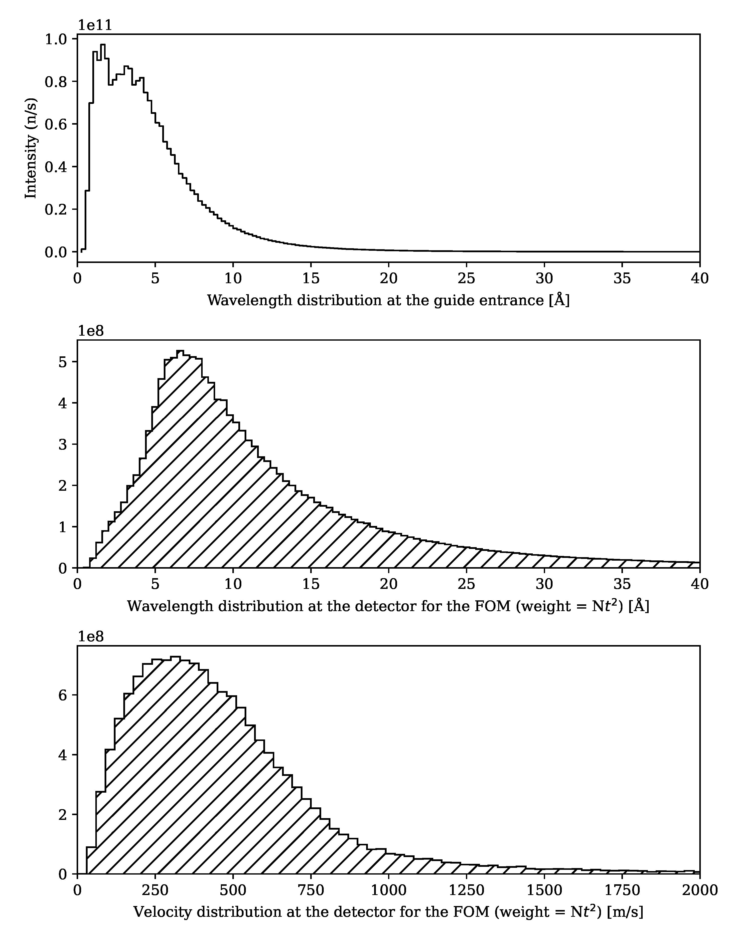
In Figure 2, we show the neutron wavelength and velocity distribution at the guide exit, both weighted using the FOM defined in Equation (36), for the configuration with the exit window of 1 m${}^2$ and a 75 m-long guide. The important feature to notice is that no wavelength cut-off is present in the distribution and the contribution of low energy neutrons stays relevant even when the source absolute intensity drastically drops, as expected by the $t^2$ factor in the calculation of the FOM (see Equation (36)).

5. Design of the $\overline{\mathit{n}}$ Annihilation Detector

Using the $n/\overline{n}$ guide simulations and the geometrical constraints in the experimental zone of PF1B, we estimate the external size of the annihilation detector in both directions to be below ∼2.8 m.

The maximum sensitivity of the experiment is achieved when the expected background is well below one event for the duration of the complete experiment and the efficiency of detection of $\overline{n}$ is maximized. A conservative estimation is that a new annihilation detector should at least achieve the 52% detection efficiency of the previous ILL [14] experiment, but most likely, due to the use of new technologies, it is expected to surpass it.

The detector must be sensitive to the characteristic antineutron–nucleon annihilation signal. The final state consists mainly of charged pions and photons from neutral pion decays. The detector consists of a thin (∼100 $\mathsf{\mu }$m) carbon foil in which the $\overline{n}$ would annihilate a tracking chamber, which will allow particle identification as well as determination of the primary vertex, and a calorimeter.

The tracking chamber will consist mainly of a Time Projection Chamber (TPC), which will provide three-dimensional tracking and a measurement of the mean energy loss $\frac{dE}{dx}$. The calorimeter comprises arrays of plastic scintillators and lead-glass modules. The primary function of the scintillators will be to identify hits originating outside the inner detector volume, which will be important for particle identification via range determinations and for the rejection of cosmic ray background events. Electromagnetic calorimetry is provided by lead-glass modules and uses the Cerenkov effect. A high precision electromagnetic calorimeter is needed to identify neutral pion production via the decay ${\pi }^0\to \gamma \gamma$. The calorimeters would be position sensitive, with a segmentation to be determined by simulation. This design is therefore in essence the same as being planned for the HIBEAM experiment at the European Spallation source [29]. A simulation and analysis software framework [30], which is based on detector simulation using Geant-4 [31,32,33], can also be used for a search at the ILL. A complete analysis with simulated datasets is beyond the scope of this work. Here, distributions of sensitive observables in signal and one of the major sources of background (cosmic ray muons) are shown to demonstrate that a feasible detector design concept exists.

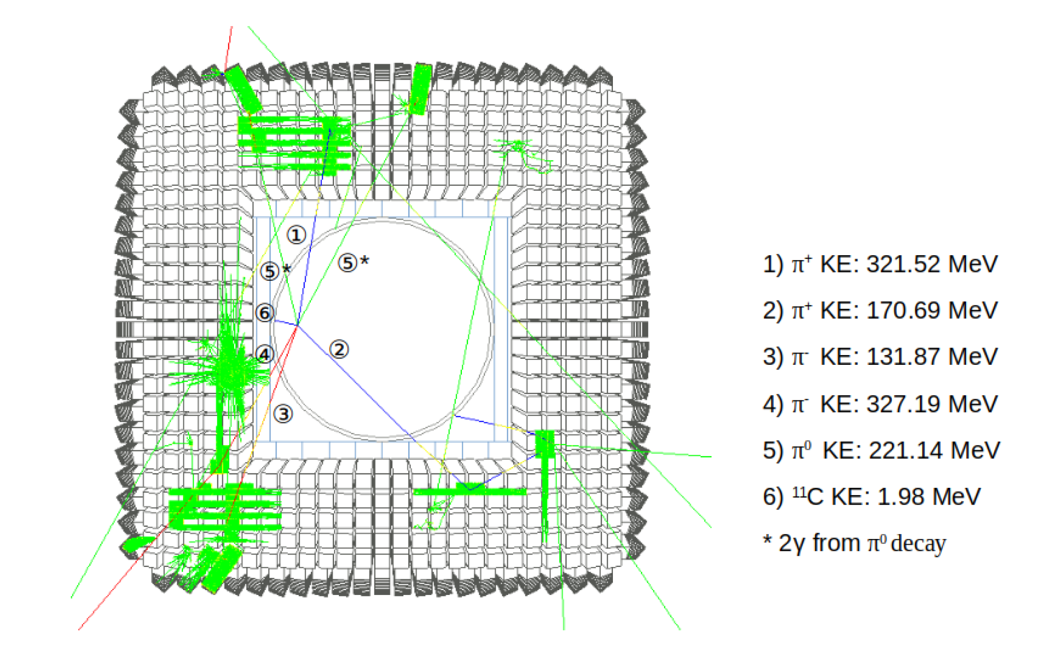
Figure 3 (top) shows a signal event with five final-state pions in the ILL detector with a nuclear fragment from the carbon target. The pions’ kinetic energies range from around 220–320 MeV. The antineutron–carbon annihilation signal was calculated with the model in Refs. [34,35].

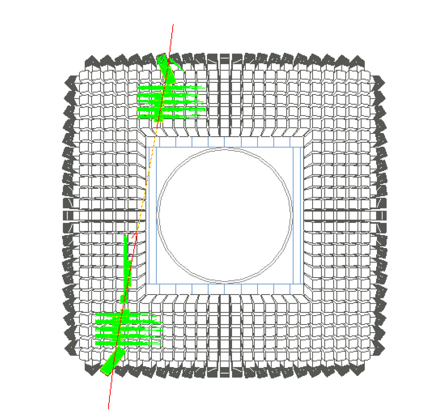
Figure 3 (bottom) shows a cosmic muon of kinetic energy 495 MeV impinging the ILL detector. The cosmic muon enters from the top detector module and leaves the detector from the bottom. This was made using the CRY [36] cosmic ray program.

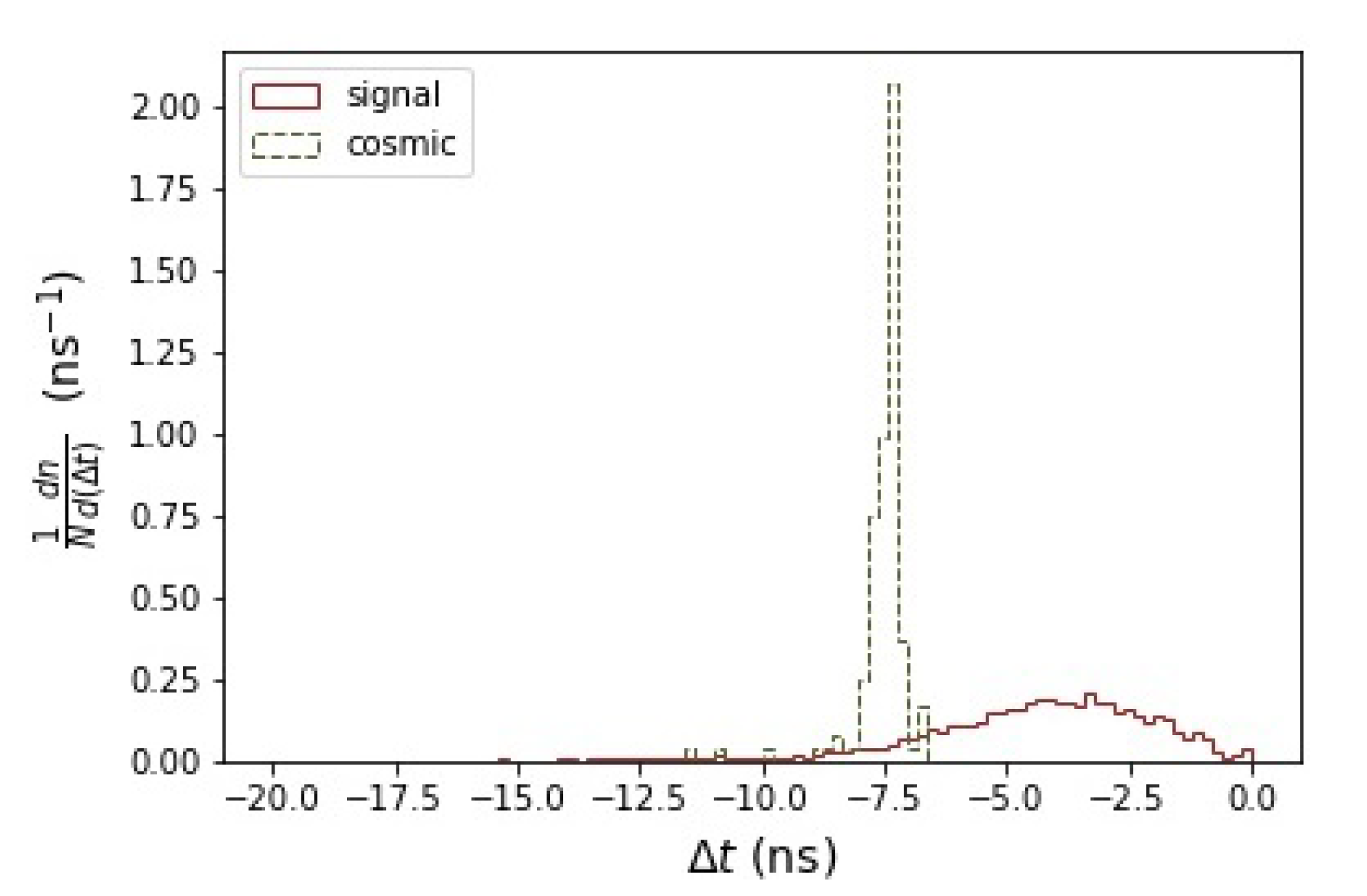
Figure 4 shows the quantity $\Delta t=t_2-t_1$, defined as the difference between the timing of the first ($t_1$) and last ($t_2$) signal in the scintillators. The spectra are shown for an annihilation event and a cosmic muon background event. Each cosmic event contains one charged cosmic muon passing through the ILL detector. Since the cosmic muons cross the top and bottom of the detector, $\Delta t$ for cosmic background is expected to be larger than the signal. As expected, clear separation between the two distributions is observed.

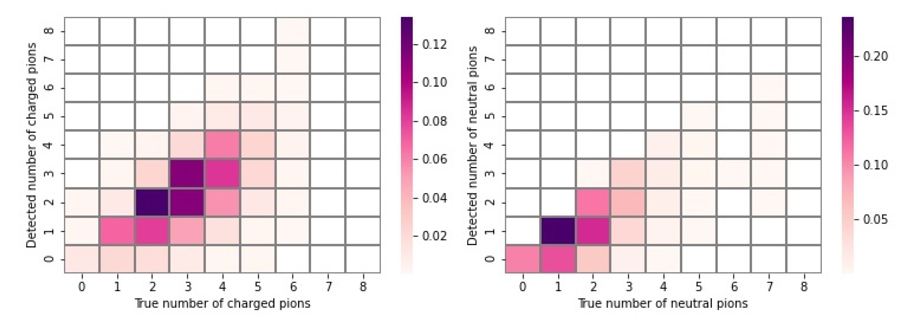
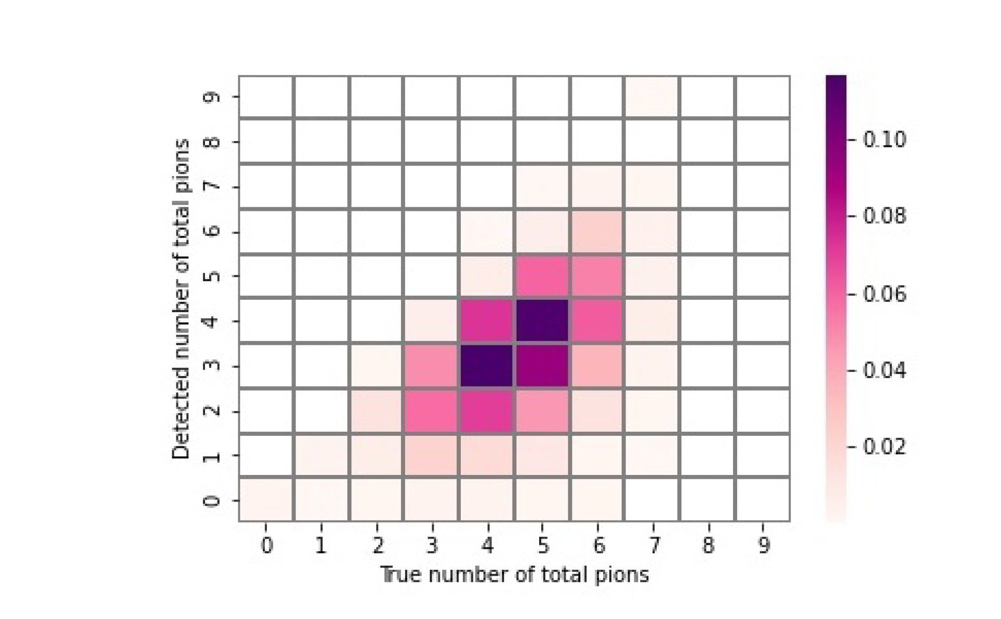
Figure 5 shows the multiplicities of neutral and charged pions for 1500 annihilation events. Measurements of pion multiplicity represent important evidence that an annihilation event has occurred.

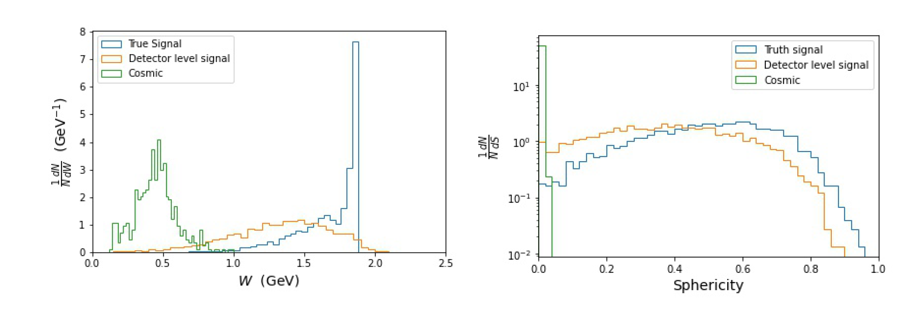
Figure 6 (Left) shows the invariant mass distributions annihilation events at truth level and at detector level, i.e., using information available from the detector such as energy loss and particle range. Detector-level background predictions for cosmic muons misidentified as pions are also shown for single muon events. The truth level invariant mass has a peak 1.88 GeV while the distribution of the reconstructed invariant is spread broadly and has a peak around 1.45 GeV in the ILL detector. The cosmic muon event distribution has a far lower invariant mass (typically around 500 MeV).

Figure 6 (Right) shows the sphericity distribution calculated for the same sets of events as shown in Figure 6 (Left). As expected, the pure cosmic ray events have small values of sphericity, closer to zero, while signal (and signal with cosmic) events have larger sphericity.

6. Conclusions

We explore the feasibility of an experiment to search for $n-\overline{n}$ oscillations at the PF1B instrument at ILL. The main gain factors over the best experiment performed earlier at PF1 instrument at ILL are: a stronger neutron beam and a new operating mode based on coherent n and $\overline{n}$ mirror reflections. We show that the overall configuration is feasible. Due to the relatively short length available at PF1B, systematic uncertainties of the method are negligible. Virtually all subcritical $\overline{n}$ would be transported without losses to the annihilation detector. A major fraction of all the initial n could be converted to subcritical ones in a special diverging $n/\overline{n}$ neutron guide.

All the following estimations are preliminary, and a more precise future analysis can change them slightly. The estimated statistical sensitivity for the $n-\overline{n}$ transition rate is up to an order of magnitude higher than that in the best performed experiment [14]. As a conservative estimate, the gain factor is ∼2.8 for the “short” neutron guide and the middle-size $\overline{n}$ detector of 1 m, see Table 1. Potentially, it can be further improved by a longer measuring time (say, a factor of ∼2), a more efficient $\overline{n}$ annihilation detector, a longer $n/\overline{n}$ guide (a factor of ∼1.6, see Table 1), a more accurate consideration of n and $\overline{n}$ transport and the account of their interaction with the guide walls (say, a factor of ∼1.3), giving all together an additional gain factor of ∼4.1), or the total gain factor of up to ∼10.

This is large enough to provide a discovery potential. If, however, the actual transition rate is beyond the sensitivity of this experiment, it would be a significant step towards a future more sensitive larger-scale experiment at the ESS [13]. It would allow one to test the main experimental approaches and components of a future experimental setup. In such an experiment, the length can be increased using a guide with a constant cross section that is put after the diverging part of the $n/\overline{n}$ guide. This would lead to a nearly quadratic gain with regard to the increased length in the experimental sensitivity, as far as $\overline{n}$ annihilation losses are not too large. Such a saturation of the sensitivity corresponds to experiment lengths much larger, or neutron spectra much softer than those considered in this paper.

The new proposed experimental scheme based on the coherent reflection of both n and $\overline{n}$ from the walls of the $n/\overline{n}$ guide, allows us to reduce the transverse size of the experiment, and therefore to reduce its cost and simplify the limitations associated with the need to provide very low magnetic fields and high vacuum, as well as to develop the annihilation detector.

The gain factor estimated in this article compares the sensitivity of the experiment [14] at PF1 and the possible sensitivity of a future experiment at PF1B. However, the same idea of coherent reflection of n and $\overline{n}$ can be also applied to the analysis of the already performed experiment [14]. The fact is that, as noted by one of the referees of this article, it contained an initial focusing section of a neutron guide 33.6 m long. It effectively increases the length of the experiment and therefore increases the sensitivity of the experiment. This result will be presented separately when the corresponding calculations are performed.