Abstract
The goal of this study was to show how a modified variational inclusion problem can be solved based on Tseng’s method. In this study, we propose a modified Tseng’s method and increase the reliability of the proposed method. This method is to modify the relaxed inertial Tseng’s method by using certain conditions and the parallel technique. We also prove a weak convergence theorem under appropriate assumptions and some symmetry properties and then provide numerical experiments to demonstrate the convergence behavior of the proposed method. Moreover, the proposed method is used for image restoration technology, which takes a corrupt/noisy image and estimates the clean, original image. Finally, we show the signal-to-noise ratio (SNR) to guarantee image quality.
1. Introduction
As technology advances, several new and challenging real-world problems develop. These problems appear in a variety of fields, such as chemistry, engineering, biology, physics, and computer science. The problems can be formulated as optimization problems, i.e., to find x such that the following holds:
where is continuously differentiable. In solving these problems, optimization and control methodologies and techniques are certainly required. Since symmetry appears in certain natural and engineering systems, there is some form of symmetry in many mathematical models and optimization problems. Therefore, researchers have to pay attention to adjusting certain constrained optimization problems, where certain variables appear symmetrically in the objective and constraint functions. One of the basic optimization concepts for finding minimization is the variational inclusion problem (VIP), which is to find x in a real Hilbert space H, such that the following holds:
where operators and are, respectively, single-valued and multi-valued. The solution of the VIP can apply to real-world problems, such as engineering, economics, machine learning, equilibrium, image processing, and transportation problems [1,2,3,4,5,6,7]. An increasing number of researchers have investigated methods to solve the variational inclusion problem. A popular one is the forward–backward splitting method (see [8,9,10]), given by the following:
where with . Moreover, researchers have modified these methods not only with more versatility by using relaxation techniques (see [11,12]), but also with more acceleration by using the inertial techniques (see [13,14,15,16]). Later, Alvarez and Attouch [14,15] expanded the inertial idea and introduced the inertial forward–backward method given by the following:
The technique of speeding up this method consists in the term . The inertial term with an extrapolation factor is well known (for more details, see [17,18,19,20]). For monotone inclusions/non-smooth convex minimization problems, they also proved the convergence theorem. Attouch and Cabot [21,22] established relaxed inertial proximal algorithms by using both techniques to increase the performance of algorithms to solve the previous problems. Later, many researchers focused on both techniques and introduced the relaxed inertial forward–backward algorithm [23], the inertial Douglas–Rachford algorithm [24], a Tseng extragradient method in Banach spaces [25], and the relaxed inertial Tseng’s type algorithm [26]. Among the well-known algorithms is the relaxed inertial Tseng’s type method developed by Abubakar et al. [26]. They solved the problem (2) by modifying Tseng’s forward–backward forward splitting approach by employing the relaxation parameter and the inertial extrapolation factor . Their algorithm is given by the following:
A new simple step size rule was designed to self-adaptively update the step size . Furthermore, they proved a weak convergence theorem generated by their algorithm and applied the algorithm to solve the problem of image deblurring.
In 2014, Khuangsatung and Kangtunyakarn [27,28] presented the modified variational inclusion problem (MVIP), that is, to find such that the following holds:
where, for every with , operator and . Obviously, if for every , then reduce from (3) to (2), and the iterative methods are used for solving a finite family of nonexpansive mappings of fixed point T and a finite family of variational inclusion problems in Hilbert spaces under the condition Their method is given by the following:
Moreover, their iterative method provided a strong convergence theorem, which they proved. Apart from that, there is another technique that can reduce the overall computational effort under widely used conditions. That is the parallel technique (for more details, see [29,30,31]). Cholamjiak et al. recently proposed an inertial parallel monotone hybrid method that solves the common variational inclusion problems. Their method is given by the following:
The idea of the parallel technique is to find the farthest element from the previous approximation They demonstrated that the method yielded strong convergence results and applied their results to solve image restoration problems.
Inspired by the ideas of [26,28,31], we provide a new method for determining the solution set of the modified variational inclusion problem in Hilbert spaces. For obtaining high performance, our method modifies the relaxed inertial Tseng’s type method by using the condition and the parallel technique, which finds the farthest element . Furthermore, under appropriate conditions, we prove a weak convergence theorem and present numerical experiments to demonstrate convergence behavior. Finally, the image restoration problems are solved by our result.
2. Preliminaries
Throughout the paper, we suppose that H is a real Hilbert space with norm and the inner product and that C is a nonempty closed and convex subset of In this section, we go over several fundamental concepts and lemmas that are utilized in the main result section.
Lemma 1.
[32] The following statements are accurate:
- (i)
- for every ;
- (ii)
- for every ;
- (iii)
- for every with
Definition 1.
Suppose that . For any ,
A is a monotone mapping if the following holds:
A is L-Lipschitz continuous if there is a constant as follows:
We mention a mapping . If and for every , then If is monotone and every implies that for every , it is called the maximal monotone.
Definition 2.
The resolvent operator associated with B is referred to as the following:
where is the maximal monotone, and I and λ are an identity mapping and a positive number, respectively.
Lemma 2.
[9] Let be a monotone Lipschitz continuous mapping, and be a maximal monotone operator; then, is the maximal monotone.
Lemma 3.
[33] Let Γ be a non empty subset of H, and a sequence of elements of Assume the following:
- (i)
- For every exists;
- (ii)
- Every weak sequential limit point of , as , belongs to
Then converges weakly as to a point in
Lemma 4.
[34] Suppose that and are sequences in . For every there is with and
Then the following conditions are satisfied:
- (i)
- where ;
- (ii)
- there is with
3. Main Results
Two algorithms are presented in this section. First, we propose Algorithm 1, which is known as a modified Tseng method for solving the modified variational inclusion problem. After that, we prove a weak convergence theorem by using some symmetry properties. Assume the following assumptions to be correct for the purposes of the investigation.
Assumption 1.
The feasible set of the VIP is a nonempty closed and convex subset of
Assumption 2.
The solution set Γ of the MVIP is nonempty.
Assumption 3.
is monotone and -Lipschitz continuous on H for every i, and is the maximal monotone.
| Algorithm 1 (Modified Tseng’s method for solving the MVIP) |
| Pick Iterative steps: Given iterates and in Step 1. Set as Step 2. Compute If stop. is the solution of MVIP. Else, go to Step 3. Step 3. Compute Set , and go back to Step 1. |
Lemma 5.
The sequence is bounded below.
Proof.
Since is -Lipschitz continuous for , we have
By (7), if for , then the following holds:
Thus, the sequence is bounded below by for .
In the case of for , it is obvious that the sequence is bounded below by . We can conclude that □
Remark 1.
According to Lemma 5, it is easy to see that the sequence is monotonically decreasing and bounded below by This implies that the update (7) is well defined and the following holds:
Lemma 6.
Let be a sequence generated by Algorithm 1. If there is a subsequence with weak convergence to q with then
Proof.
We assume that , which means By we have the following:
Therefore, Because B is the maximal monotone, we obtain the following:
Hence,
Since is -Lipschitz continuous and it follows that If exists, it receives the following:
Based on the maximal monotonicity of and (11), a zero is in We can conclude that □
Theorem 1.
Assume the following:
with and If every then generated by Algorithm 1 converges weakly to .
Proof.
We know that the resolvent is firmly non-expansive and
Thus, we have the following:
Obviously, This implies that
However, To replace the previous equation in (13), we obtain the following:
The definition of implies the following:
for each Consider the following:
Substituting (16) in (15), we obtain the following:
for each Putting (14) in (17), we obtain that, for every
where By the definition of and (10), it follows that
for every The following can be stated:
From (19), it follows that
Therefore,
We also can state the following:
Obviously, with as , we have the following:
By the definition of , we have the following:
By the Cauchy–Schwartz inequality, it follows that
Therefore,
We note the following:
Thus,
where By the assumption of (12), we obtain This indicates that is nonincreasing. Furthermore, we have the following:
and
It follows that
Taking in the previous equation, we have It can be concluded that We consider the following:
For solving the problem of (2), the following algorithm (Algorithm 2) is suggested when setting in Algorithm 1
| Algorithm 2 (Modified Tseng’s method for solving the VIP) |
| Pick Iterative steps: Given iterates and in Step 1. Set as Step 2. Compute If stop. is the solution of the VIP. Else, go to Step 3. Step 3. Compute The stepsize sequence is updated as follows: Set , and go back to Step 1. |
Corollary 1.
If the solution set of the VIP is nonempty, then the sequence generated by Algorithm 2 converges weakly to .
Proof.
Proofs are similar by setting in Lemma 5, 6, and Theorem 1. □
4. Numerical Experiments
We provide numerical examples to demonstrate the behavior of our algorithm in this section. We have broken it down into two examples.
The behavior of an error of the sequence generated by Algorithm 1 is demonstrated in Example 1. Furthermore, in Example 1, we demonstrate the behavior of the sequence , which is generated by Algorithm 1 by separating the dimension of the sequence .
In Example 2, we apply our main result to solve image deblurring problems. Image recovery problems could be explained using the inversion of the following observation model:
where M is a deblurring matrix, represents the original image, b is the deblurring image, and is the Gaussian noise. The convex unconstrained optimization problem is known to be the same as solving (39):
as the regularization parameter . For solving (40), we suppose and , where and . Therefore, is -cocoercive. This implies that is nonexpansive and that . Because is the maximal monotone, x is an (40) solution if and only if the following holds:
In addition, we might still formulate (40) as a convex constrained optimization problem for the split feasibility problem (SFP):
where is a given constant and (41) is solved. Setting , we consider and We use Algorithm 1 to solve this image deblurring problem. Figure 1 shows a flowchart of the technique for selecting a blurring function A by summing N blurring functions .
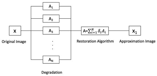
Figure 1.
The flowchart of the image restoration process.
Example 1.
Let be a two-dimensional space of real numbers. Define monotone operators , and maximal monotone operator for every . Moreover, we set parameters , and and choose the initial point as and . For the time being, it is exciting to see that all of our parameters and operators are satisfied with our main result. By applying Algorithm 1, we can solve the problem of (3) and show the behavior of our algorithm.
After completion the experiment, we can observe that a sequence always converges to the solution point of the problem of (3), independently of the arbitrary starting point.
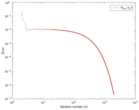
In Figure 2, we plot the error graph of a sequence . This shows that the sequence achieves a small error when the number of iterations is higher. We are also confident that increasing the number of iterations will result in an inaccuracy of less than .
Figure 2.
Error plot of Algorithm 1.
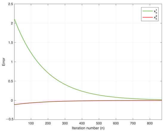
In Figure 3, we plot the sequence by separating dimension of . We can conclude that a sequence always converges to the solution of the interested problem. That is, as .
Figure 3.
Plot of the sequence by separating dimensions of .
Furthermore, the detailed analysis of the computations of our algorithm is shown in Table 1 for and for all .

Table 1.
Detailed analysis of computational of Algorithm 1.
Example 2.
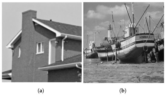
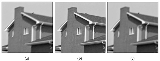
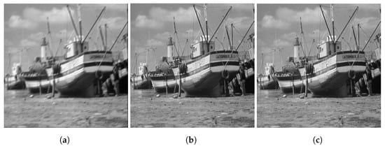
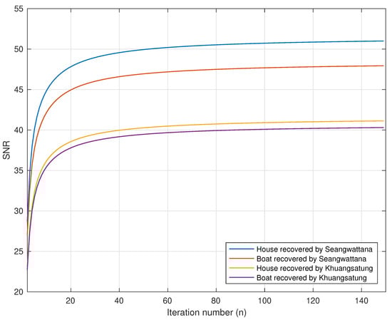
As the blurring function, we used MATLAB’s motion blur by using as fspecial (’motion’,9,40) and as fspecial (’gaussian’,9,2). The standard test images of a house and of boats are used in the comparison (see Figure 4). We compare our proposed algorithm (Algorithm 1) with the algorithm in [28]. The control parameters are set as follows: , and . The results of this experiment can be seen in Figure 5, Figure 6 and Figure 7. To analyze the image quality that is restored, we adopted the signal-to-noise ratio (SNR) as follows:
where x is the original image, and is the estimated image at iteration n. In Figure 7, the SNR values of the house and boat images restored by Algorithm 1 (Figure 5b and Figure 6b) are higher than those images restored by the algorithm in [28] (Figure 5c and Figure 6c). The superiority of the proposed algorithm in measures of SNR is shown.
Figure 4.
Original test images: (a) House and (b) Boats.
Figure 5.
(a) Degraded house image, (b) house image restored by Algorithm 1; (c) house image restored by the algorithm in [28].
Figure 6.
(a) Degraded boats image; (b) boats image restored by Algorithm 1; (c) boats image restored by the algorithm in [28].
Figure 7.
SNR values of the house and boats images restored by Algorithm 1 and the algorithm in [28].
5. Conclusions
Two modified Tseng’s methods are presented for solving the modified variational inclusion and the variational inclusion problems by using the condition for the modified variational inclusion problems and the parallel technique. Additionally, we demonstrate the behavior of our algorithm and use it to solve image deblurring problems.
Author Contributions
Conceptualization, K.S. (Kanokwan Sitthithakerngkiet); formal analysis, T.S.; funding acquisition, T.S.; investigation, K.S. (Kanokwan Sitthithakerngkiet); methodology, T.S.; software, K.S. (Kanokwan Sitthithakerngkiet); validation, T.S., K.S. (Kamonrat Sombut) and A.A.; visualization, K.S. (Kanokwan Sitthithakerngkiet); writing—original draft, T.S.; writing—review & editing, K.S. (Kanokwan Sitthithakerngkiet). All authors have read and agreed to the published version of the manuscript.
Funding
This research was funded by National Science, Research and Innovation Fund (NSRF), King Mongkut’s University of Technology North Bangkok with Contract No. KMUTNB-FF-65-13.
Acknowledgments
The authors would like to thank King Mongkut’s University of Technology North Bangkok (KMUTNB), Rajamangala University of Technology Thanyaburi (RMUTT) and Nakhon Sawan Rajabhat University. We appreciate the anonymous referee’s thorough review of the manuscript and helpful suggestions for refining the presentation.
Conflicts of Interest
The authors declare no conflict of interest.
References
- Baiocchi, C. Variational and Quasivariational Inequalities. In Applications to Free-Boundary Problems; Springer: Basel, Switzerland, 1984. [Google Scholar]
- Byrne, C. A unified treatment of some iterative algorithms in signal processing and image reconstruction. Inverse Probl. 2004, 20, 103–120. [Google Scholar] [CrossRef]
- Marcotte, P. Application of Khobotov’s algorithm to varaitional inequalities and network equilibrium problems. INFOR Inf. Syst. Oper. Res. 1991, 29, 258–270. [Google Scholar]
- Hanjing, A.; Suantai, S. A fast image restoration algorithm based on a fixed point and optimization method. Mathematics 2020, 8, 378. [Google Scholar] [CrossRef]
- Gibali, A.; Thong, D.V. Tseng type method for solving inclusion problems and its applications. Calcolo 2018, 55, 49. [Google Scholar] [CrossRef]
- Thong, D.V.; Cholamjiak, P. Strong convergence of a forward-backward splitting method with a new step size for solving monotone inclusions. Comput. Appl. Math. 2019, 38, 94. [Google Scholar] [CrossRef]
- Khobotov, E.N. Modification of the extra-gradient method for solving variational inequalities and certain optimization problems. USSR Comput. Math. Math. Phys. 1987, 27, 120–127. [Google Scholar] [CrossRef]
- Tseng, P. A modified forward-backward splitting method for maximal monotone mappings. SIAM J. Control Optim. 1998, 38, 431–446. [Google Scholar] [CrossRef]
- Lions, P.L.; Mercier, B. Splitting algorithms for the sum of two nonliner operators. SIAM J. Numer. Anal. 1979, 16, 964–979. [Google Scholar] [CrossRef]
- Passty, G.B. Ergodic convergence to a zero of the sum of monotone operators in Hilbert space. J. Math. Anal. Appl. 1979, 72, 383–390. [Google Scholar] [CrossRef]
- Bauschke, H.H.; Combettes, P.L. Convex Analysis and Monotone Operator Theory in Hilbert Spaces; Springer: New York, NY, USA, 2011. [Google Scholar]
- Eckstein, J.; Bertsekas, D. On the Douglas-Rachford splitting method and the proximal point algorithm for maximal monotone operators. Math. Program. 1992, 55, 293–318. [Google Scholar] [CrossRef]
- Nesterov, Y. A method for unconstrained convex minimization problem with the rate of convergence O(). Doklady Ussr. 1983, 269, 543–547. [Google Scholar]
- Alvarez, F. On the minimizing property of a second order dissipative system in Hilbert spaces. SIAM J. Control Optim. 2000, 38, 1102–1119. [Google Scholar] [CrossRef]
- Alvarez, F.; Attouch, H. An inertial proximal method for maximal monotone operators via discretization of a nonlinear oscillator with damping. Set-Valued Anal. 2001, 9, 3–11. [Google Scholar] [CrossRef]
- Abubarkar, J.; Kumam, P.; Rehman, H.; Ibrahim, A.H. Inertial iterative schemes with variable step sizes for variational inequality problem involving pseudo monotone operator. Mathematics 2020, 8, 609. [Google Scholar] [CrossRef]
- Ceng, L.C.; Petrusel, A.; Qin, X.; Yao, J.C. A Modified inertial subgradient extragradient method for solving pseudomonotone variational inequalities and common fixed point problems. Fixed Point Theory 2020, 21, 93–108. [Google Scholar] [CrossRef]
- Ceng, L.C.; Petrusel, A.; Qin, X.; Yao, J.C. Two inertial subgradient extragradient algorithms for variational inequalities with fixed-point constraints. Optimization 2021, 70, 1337–1358. [Google Scholar] [CrossRef]
- Zhao, T.Y.; Wang, D.Q.; Ceng, L.C.; He, L.; Wang, C.Y.; Fan, H.L. Quasi-inertial Tseng’s extragradient algorithms for pseudomonotone variational inequalities and fixed point problems of quasi-nonexpansive operators. Numer. Funct. Anal. Optim. 2020, 42, 69–90. [Google Scholar] [CrossRef]
- He, L.; Cui, Y.L.; Ceng, L.C.; Wang, D.Q.; Hu, H.Y. Strong convergence for monotone bilevel equilibria with constraints of variational inequalities and fixed points using subgradient extragradient implicit rule. J. Inequal. Appl. 2021, 146, 1–37. [Google Scholar] [CrossRef]
- Attouch, H.; Cabot, A. Convergence of a relaxed inertial proximal algorithm for maximally monotone operators. Math. Program. 2020, 184, 243–287. [Google Scholar] [CrossRef]
- Attouch, H.; Cabot, A. Convergence rate of a relaxed inertial proximal algorithm for convex minimization. Optimization 2019, 69, 1281–1312. [Google Scholar] [CrossRef]
- Attouch, H.; Cabot, A. Convergence of a relaxed inertial forward-backward algorithm for structured monotone inclusions. Appl. Math. Optim. 2019, 80, 547–598. [Google Scholar] [CrossRef]
- Bot, R.I.; Csetnek, E.R.; Hendrich, C. Inertial Douglas-Rachford splitting for monotone inclusion problems. Appl. Math. Comput. 2015, 256, 472–487. [Google Scholar]
- Oyewole, O.K.; Abass, H.A.; Mebawondu, A.A.; Aremu, K.O. A Tseng extragradient method for solving variational inequality problems in Banach spaces. Numer. Algor. 2021, 1–21. [Google Scholar] [CrossRef]
- Abubakar, A.; Kumam, P.; Ibrahim, A.H.; Padcharoen, A. Relaxed inertial Tseng’s type method for solving the inclusion problem with application to image restoration. Mathematics 2020, 8, 818. [Google Scholar] [CrossRef]
- Khuangsatung, W.; Kangtunyakarn, A. Algorithm of a new variational inclusion problem and strictly pseudononspreading mapping with application. Fixed Point Theory Appl. 2014, 209. [Google Scholar] [CrossRef]
- Khuangsatung, W.; Kangtunyakarn, A. A theorem of variational inclusion problems and various nonlinear mappings. Appl. Anal. 2018, 97, 1172–1186. [Google Scholar] [CrossRef]
- Anh, P.K.; Hieu, D.V. Parallel and sequential hybrid methods for a finite family of asymptotically quasi ϕ-nonexpansive mappings. J. Appl. Math. Comput. 2015, 48, 241–263. [Google Scholar] [CrossRef]
- Anh, P.K.; Hieu, D.V. Parallel hybrid iterative methods for variational inequalities, equilibrium problems and common fixed point problems. Vietnam J. Math. 2016, 44, 351–374. [Google Scholar] [CrossRef]
- Cholamjiak, W.; Khan, S.A.; Yambangwai, D.; Kazmi, K.R. Strong convergence analysis of common variational inclusion problems involving an inertial parallel monotone hybrid method for a novel application to image restoration. Rev. Real Acad. Cienc. Exactas Fis. Nat. Ser. Mat. 2020, 114, 351–374. [Google Scholar] [CrossRef]
- Takahashi, W. Nonlinear Function Analysis; Yokohama Publishers: Yokohama, Japan, 2000. [Google Scholar]
- Opial, Z. Weak convergence of the sequence of successive approximations for nonexpansive mappings. Bull. Am. Math. Soc. 1967, 73, 591–597. [Google Scholar] [CrossRef]
- Ofoedu, E.U. Strong convergence theorem for uniformly L-Lipschitzian asymptotically pseudo contractive mapping in real Banach space. J. Math. Anal. Appl. 2006, 321, 722–728. [Google Scholar] [CrossRef]


Publisher’s Note: MDPI stays neutral with regard to jurisdictional claims in published maps and institutional affiliations. |
© 2021 by the authors. Licensee MDPI, Basel, Switzerland. This article is an open access article distributed under the terms and conditions of the Creative Commons Attribution (CC BY) license (https://creativecommons.org/licenses/by/4.0/).