Spectral Clustering Effect in Software Development Effort Estimation

Abstract

Software development effort estimation is essential for software project planning and management. In this study, we present a spectral clustering algorithm based on symmetric matrixes as an option for data processing. It is expected that constructing an estimation model on more similar data can increase the estimation accuracy. The research methods employ symmetrical data processing and experimentation. Four experimental models based on function point analysis, stepwise regression, spectral clustering, and categorical variables have been conducted. The results indicate that the most advantageous variant is a combination of stepwise regression and spectral clustering. The proposed method provides the most accurate estimates compared to the baseline method and other tested variants.

1. Introduction

The key role of project management is to estimate an effort to develop software projects. In this article, selected methods for estimating the development effort of software projects are addressed. Software development suffers from poor project management and consequently poor budgeting. Development effort and budgeting should then be correlated—symmetrical to software size. Software size is a value of software complexity. It is measured in various units; function points, use case points, lines of codes, etc. [1,2,3,4].

Software size estimation can be done by using several methods [1] that utilize different classification approaches [1,2,3,4]. In this paper, an algorithmic method called function point analysis (FPA) is used. FPA is standardized according to ISO [5]. The FPA method depends on the capabilities and experiences of the analysts, who are responsible for the processing and evaluation of parameters [6]. The software system size is obtained using a set of functions, which evaluate selected parameters described by the system analyst.

The objective of this paper is to present a study in which an algorithmic model based on FPA, spectral clustering (SC), which employs symmetric matrix and stepwise regression (SR) will be evaluated. This model is tested as an option to minimize the error of the development effort estimation (DEE). The estimation methods are based on regressions approaches which follow a normal distribution (symmetrical) of residual errors.

The remainder of this paper is divided into the following sections. Section 2 presents a related work. Section 3 defines the problem statement. Section 4 describes the methods used in this study and the experimental design. The results and discussion are presented in Section 5, and finally, Section 6 contains a conclusion.

2. Related Work

Many clustering approaches are under investigation in the scope of software effort estimation. The authors of [7] introduced a method to increase the software DEE accuracy based on the combination of fuzzy clustering and analogy methods. In [8], challenges facing the analogy-based effort estimation was presented by introducing a general fuzzy c-means method, which can handle a mixture of variables.

More than 60 papers published between 1990 and 2012 were examined by Idri et al. [9]. The majority of these research papers are centered on removing unwanted datapoints from datasets. Removing unwanted datapoints from training dataset can be performed by applying a clustering approach. Clustering aids in the discovery of parallels across projects and has been extensively researched for minimizing the quantity of historical data points and identifying the most comparable subgroups. Azzeh et al., addressed the issue of determining the number of nearby projects by using a method known as bisecting k-medoids [10]. It is demonstrated in [11] that grouping varied projects into clusters can aid to accurate assessment. In this paper is confirmed that clustering improves estimate accuracy. In [12] the authors present a hybrid model with classification and prediction phases employing a support vector machine and radial basis neural networks.

The authors of [13] established a technique for estimating equation elicitation by dividing historical project datapoints. Garre et al. [14] describe a beneficial effect of the improved expectation-maximization method (EM). Updated EM method was introduced by Dempster et al. [15]. Hihn et al. [16] proved that SC produces less outliners than the closest neighbor approach. Dataset segmentation omits inconsistent projects and improves estimation accuracy as was described by Bardisiri et al. [7]. Both [17,18] present the usage of the particle swarm optimization algorithm.

Prokopova et al. [19] showed how important it is to select the clustering type and distance metric. Furthermore, the k-means algorithm exhibits better performance than the hierarchical clustering method.

Employing clustering allows for the evaluation of project attributes for similarity. This approach supports a comparison of a new project with projects located in related clusters based on similarity measures.

The investigations of Lokan and Mendes [20] represents different approaches for searching similar projects. These researchers showed that moving windows are helpful for a subset selection technique. This approach is based on the idea that past projects, with similar finishing times, allow the creation of a better estimation model. In [21], moving windows were used in conjunction with regression models. In [22], the authors compared moving windows and SC. As shown, SC excels when compared to moving windows or the k-means approach.

Minku [23] investigated whether threshold clustering has a positive impact on estimation accuracy.

In [24], a categorical variable segmentation (CVS) model was introduced. The CVS model is based on dataset segmentation, where the relative project size (see

Table 1. Project relative size.

Group	Relative Size	Dataset Type	Size (Person-Hours)
1	XXS	Extra-extra small	>0 to <10
2	XS	Extra small	>10 to <30
3	S	Small	>30 to <100
4	M1	Medium 1	>100 to <300
5	M2	Medium 2	>300 to <1000
6	L	Large	>1000 to <3000
7	XL	Extra large	>3000 to <9000
8	XXL	Extra-extra large	>9000 to <18,000
9	XXXL	Extra-extra-extra large	>18,000

) is used as a segmentation parameter. This approach allows an estimation of the software development effort by using a specific model trained on a specific data segment. Ventura-Molina et al. [25] present an approach to work with the product delivery rate (productivity) as an important estimation parameter when a software delivery model is proposed.

3. Problem Statement

FPA, which serves as the basis for further research, is based on the set of evaluation rules for size estimation. In this study, the International Function Point Users Group (IFPUG) [26] method is used. The development effort is understood as time in person-hours, which is needed for the completion of all development tasks.

When an algorithmic approach based on IFPUG is used, the DEE is understood as a product of software size and product delivery rate (PDR). The IFPUG methods lack accuracy for new project estimation due to issues with replicability. The IFPUG method depends on the capabilities and experiences of the analysts, who are responsible for the processing and evaluation of the parameters [6]. IFPUG methods were designed for software size estimation and not for the DEE. This reveals another issue, namely, the correctness of the PDR.

In this study, a method for rendering a more accurate estimation is evaluated, and the results are presented. The main goal of the article is to evaluate the effect of SC together with SR.

The following research questions are investigated:

• RQ1: How SR will influence the DEE?
• RQ2: How will the model based on SR benefit when SC is employed? Will SC make the DEE more accurate?
• RQ3: How does the involvement of categorical variables affect DEE accuracy?

4. Materials and Methods

4.1. Dataset Pre-Processing

The experiments use data that are part of a dataset prepared by the International Software Benchmarking Standards Group (ISBSG) [27]. This dataset contains information on more than eight thousand projects. However, it is necessary to clean the dataset for the purposes of the presented research. The cleaning procedure was as follows:

• IFPUG compliance: Removing all projects that are not described from the perspective of estimation using the function point method (=IFPUG).
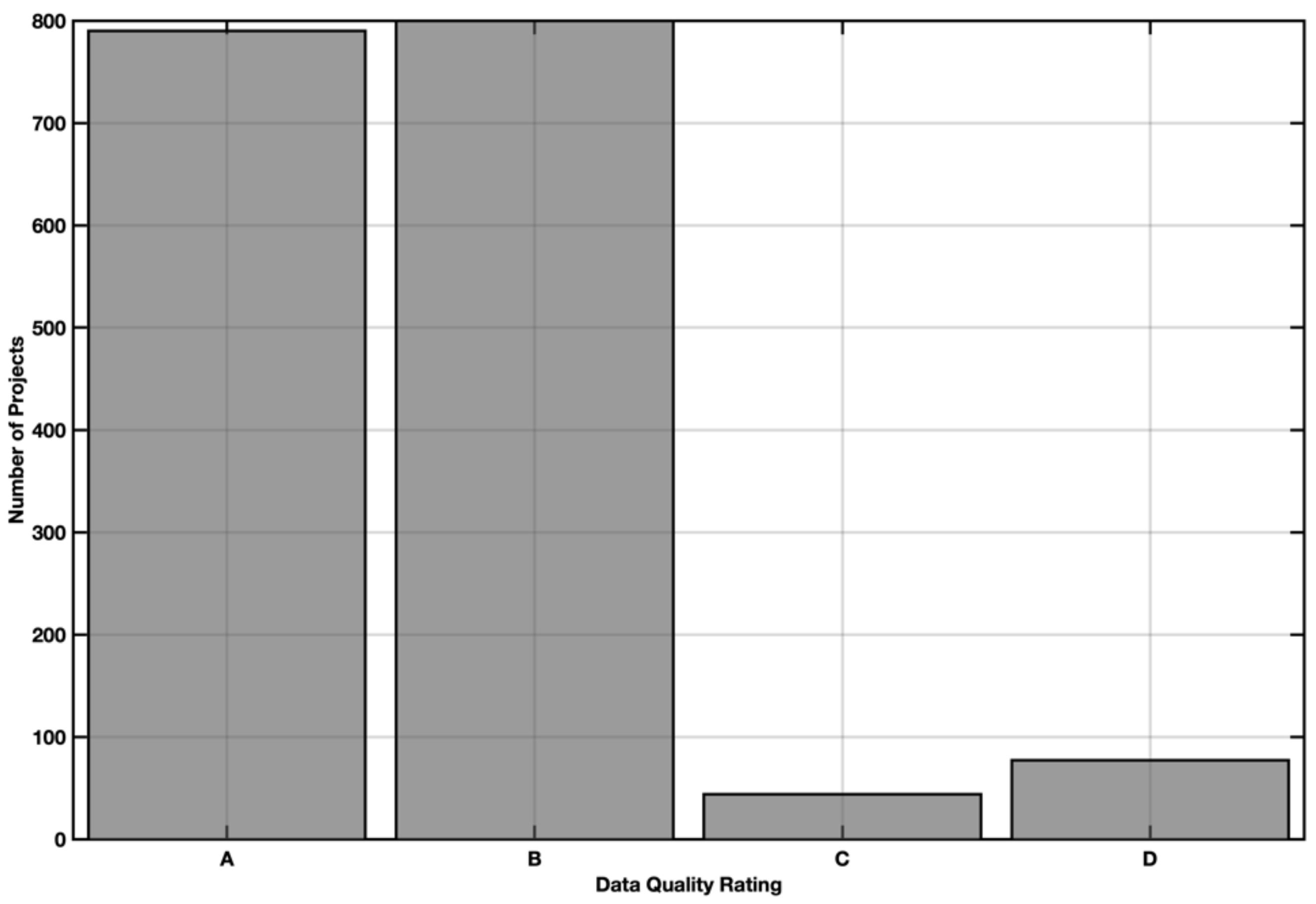
• Data quality rating: Each project is evaluated by the data quality (Figure 1). All projects having quality ratings other than A or B were removed from the working dataset.
• Value-added factor (VAF) compliance: In the next step, those projects for which the VAF was unknown were removed.
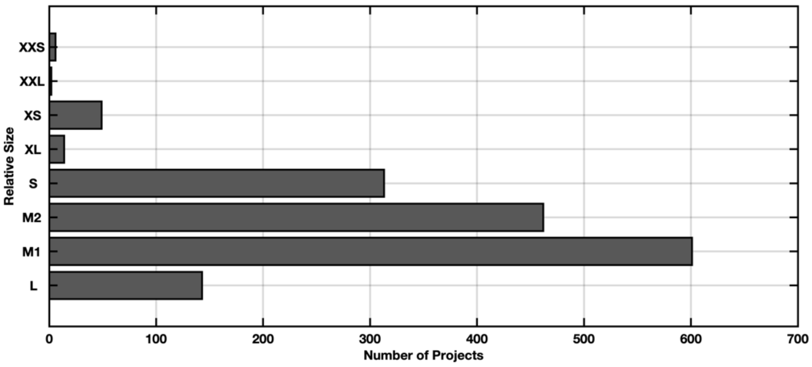
• Relative Size: Projects are classified according to size (Table 1) using the relative size variable of the projects. Projects from the extra-extra-extra-large category (XXXL) were removed.

The final working dataset contains 809 projects. Figure 2 presents a size distribution of the dataset using a relative size variable.

Table 2. Characteristics of the dataset.

Mean Value			Std. Deviation
PDR	FP	Effort	PDR	FP	Effort
19.79	358.16	5291.8	22.94	651.43	8317.07
min			max
PDR	FP	Effort	PDR	FP	Effort
0.4	6	31	259.7	13,580	71,729

summarizes the basic descriptive statistics. Three basic variables are presented:

• Productivity factor (PDR).
• Project size in function points (FPs).
• Development effort in man-hours (Effort).

The following variables are used for the study and each experiment.

• External input (EI)—requirements that define the number of external inputs.
• External output (EO)—describes the number of external outputs.
• External query (EQ)—describes the number of external queries.
• Internal logical file (ILF)—describes the number of internal logical files.
• External interface file (EIF)—describes the number of external interface files.
• Value adjustment factor (VAF)—represents the correction value that summarizes the general system characteristics (GSCs).
• Industry sector (IS)—describes the sector of the company where the project is used.
• Primary programming language (PPL)—describes the programming language used for development (C#, Java, etc.).
• Relative size (RS)—describes the project size based on the number of FPs.
• Development type (DT)—describes the project development type (new development, enhancement of existing application, etc.).
• Development platform (DP)—describes a development platform, which is the project focus (desktop, mobile, etc.).
• Development effort estimation (DEE)—represent and estimated value of effort in person-hours.
• Normalized work effort (NWE)—describes the number of person-hours required for the project.

4.2. Methods Used in Study

This study is based on IFPUG analysis of the software project size. The main goal is to evaluate whether models based on IFPUG estimate effort more accurately than the original IFPUG approach. In this study, a following methods [24] are used:

• IFPUG.
• Stepwise regression.
• Spectral clustering.
• The IFPUG method is used to elicit variables when the counting process is as follows:
• Determine the EI, EO, EQ, ILF, and EIF.
• Determine the unadjusted FP count.
• Determine the VAF.
• Determine the number of FPs.

Counting size using IFPUG means identification and classification at a complexity level. Size as the adjusted function point (AFP) is calculated using Equation (1).

$$AFP=(\sum EI\times weight+\sum EO\times weight+\sum EC\times weight+\sum EIF\times weight+\sum ILF\times weight)\times VAF$$

(1)

The weighted sums of the EI, EO, EC, EIF, and ILF are summed and then multiplied by the VAF.

Finally, the DEE in person-hours is calculated. The DEE is related to the PDR.

The PDR is used as a constant that describes the relationship between one FP and the number of hours needed for its implementation. The PDR is typically used as the mean value based on past projects or more precisely based on project type [28,29]. The PDR setting and calculation can be further studied based on [30,31].

IFPUG is described in [24], and a more extensive description may be found in the IFPUG handbook [26]. SR is utilized in the manner outlined in [24]. The method is derivate from findings and description originally presented in [22,32,33]. SR is based on adding or removing variables that involve the selection of independent variables and may be summarized as follows [22,24]:

• Create a beginning model with specified variables; alternatively create a null model.
• Establish final model limitations—establish the requested model complexity—linear, quadratic, interaction, and so on.
• Decide a control threshold—it should be the total of residual or another metric. The goal is to determine whether another variable should be eliminated or added.
• Re-testing the model after adding or eliminating variable.
• SR stops when there is no further progress in estimate.

SR creates a large number of models given a set of independent variables. The assumptions of multiple linear regression (MLR) must be met. The MLR in algebraic form (2):

$$y_i={\beta }_0+{\beta }_1{X}_{i1}+{\beta }_2{X}_{i2}+\dots +{\beta }_p{X}_{ip}+{\epsilon }_i$$

(2)

where $i=1,\dots n, y_i$ is the dependent variable; $X_{i1}\dots X_{ip}$ are predictors; ${\beta }_1\dots {\beta }_n$ are regressors; and ${\beta }_0$ is an intercept.

The residuals are represented by the value of ${\epsilon }_i$. The model is built in the form of a matrix, with each row representing a data point.

SC is employed in the manner outlined and provided in [24,34]. The approach is based on a graphical representation, where each data point is a node and the edges between data points denote similarity and is described in [16,22,34,35].

In SR, the k-nearest neighbor graph, $\epsilon$—neighborhood graph, and fully connected graph are commonly employed [36]. The k-nearest neighbor graph connects the vertices $v_i$ and $v_j$, where $v_j$ is one of $v_i$′ k-nearest neighbors. The $\epsilon$-neighbourhood graph joins all data points with pairwise distances less than $\epsilon$. The adjacency matrix $W$ (3) is as follows:

$$W=\left(w_{ij}\right)$$

(3)

where $i,j=1\dots n$ and each cell in the matrix represents the edge weight between two data points. There is no relationship between the edges if the weight is 0. After that, a Laplacian matrix (4) is computed:

$$L=D-W$$

(4)

where vertex degree $v_i$. represent the diagonal matrix $D$. An important step in SC is a spectrum calculation. It takes a form of the $L$ matrix. Normalized Laplacian algorithm is used, there are two options: a symmetric matrix (5) or a random walk (6):

$$L_{sym}=D^{-1/2}L{D}^{-1/2}=I-D^{-1/2}W{D}^{-1/2}$$

(5)

$$L_{rw}=D^{-1}L=I-D^{-1}W$$

(6)

The spectrum is a sorted list of $L, L_{sym} \mathrm{or} L_{rw}$ matrix’s eigenvectors. The eigenvectors illustrate a data point and an eigenvalue of an $L, L_{sym}, \mathrm{or} L_{rw}$ matrix. These eigenvectors are used as a feature by SC.

Finally, the clustering algorithm is applied. In this paper a k-means is utilized, but the clustering can be done by any clustering algorithm.

4.3. Experiment Settings and Configuration

In this study, a following experiments were performed.

• IFPUG (EX1).
• Stepwise regression (EX2).
• Stepwise regression and spectral clustering (EX3).
• Stepwise regression and spectral clustering + categorical variables (EX4).

4.3.1. EX1—IFPUG Base Model

Experiment EX1 represents a base model, which is used for comparison.

The estimation of effort is calculated by using the EI, EO, EQ, ILF, and EIF, which are used for the AFP (as available in the dataset).

The DEE is performed by using a PDR value, which comes as a mean on each IS group, as can be found in the dataset. More information regarding the PDR value and its elicitation based on IS can be found [24].

The DEE and NWE were later used for the estimation error (EE) calculation.

The following points summarize an EX1 process:

• Create training and testing sets by using 10-fold cross validation.
• Estimate the software size using the IFPUG (AFP) for each testing fold.
• Multiply the AFP by the industry sector-based PDR.
• Compute the EE for projects in the testing folds.
• Compute evaluation criteria—10-fold mean value.

4.3.2. EX2—Stepwise Regression

The SR method [2,32] is used to select dependent variables, which contribute to estimation accuracy. This means that the method should produce a model with the desired characteristics. The model was configured as follows:

• Independent variables: EI, EO, EQ, ILF, and EIF.
• Dependent variable: NWE.
• Criterion for SR: sum of the squared error (SSE) minimalization.

The following points summarize an EX2 process:

• Create training and testing sets by using the 10-fold procedure.
• Create a regression model using the SR procedure for each of the training folds.
• Using an obtained formula for the DEE by using and testing folds.
• Obtaining the EE for projects in the testing folds and computing them.
• Compute evaluation criteria, and a 10-fold mean value is used for comparison.

4.3.3. EX3—Stepwise Regression with Spectral Clustering

The SR method is complemented by SC [22,34] in this experiment. SC is used to search for similar projects.

Model was configured as follows:

• Independent variables: EI, EO, EQ, ILF, and EIF.
• Dependent variable: NWE.
• Criterion for SR: SSE minimalization.
• Clustering method: k-means.
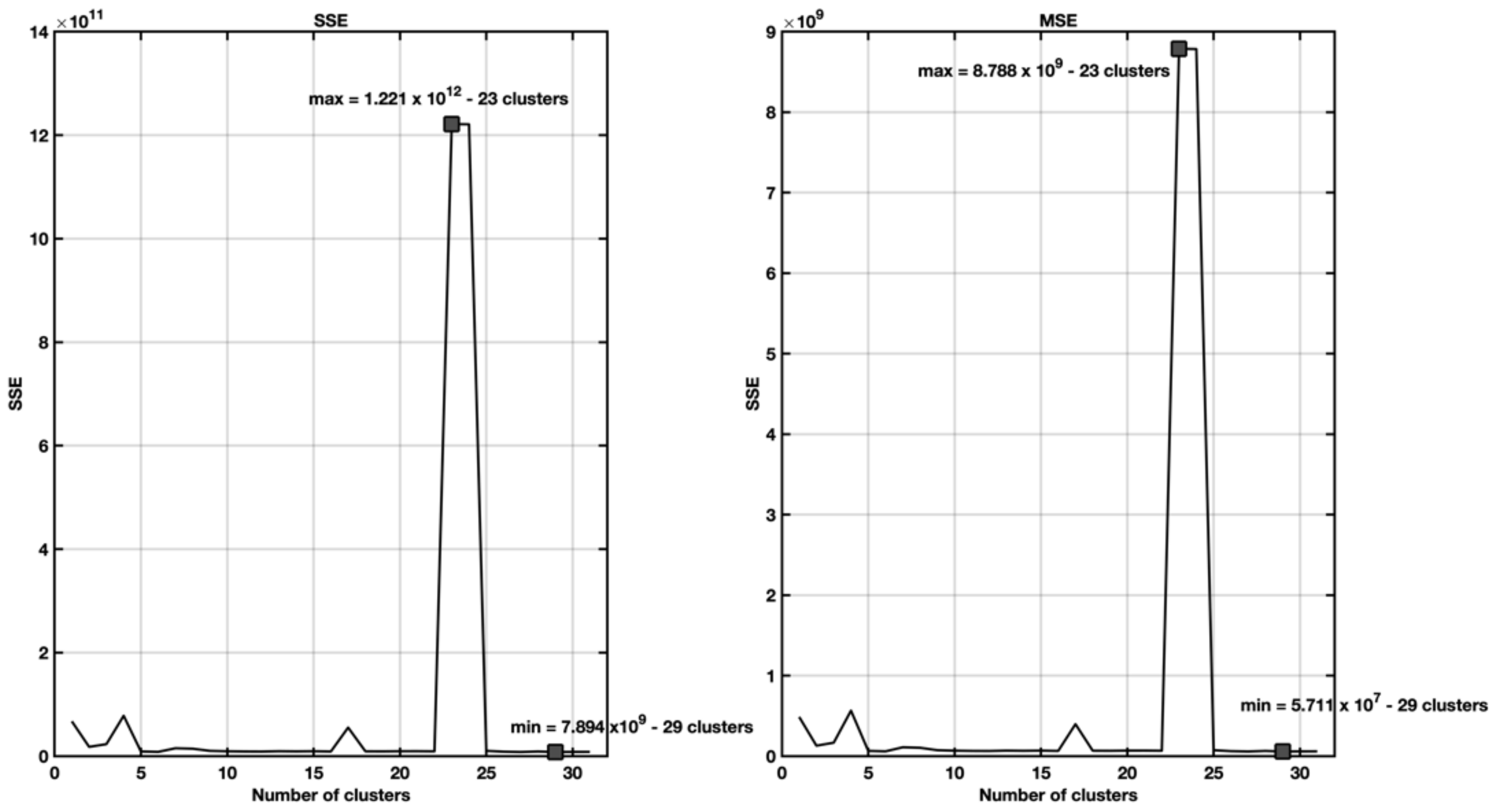
• Number of tested clusters: 2–31.
• Clustering attributes: EI, EO, EQ, ILF, and EIF.

This means that the number of clusters must be predefined before an algorithm can start. In these experiments (as in others where SR is involved) instead of hyper-parameter tuning or other known methods for selecting the proper number of clusters, a fixed interval is used to keep a cluster size within potentially usable values for regression models (not to small).

The following points summarize an EX3 process:

• Create training and testing sets by using the 10-fold procedure.
• Apply SC to the training folds.
• Computing SR models for all defined clusters.

Obtain a new estimation as follows:

• Classify observations in the testing fold into clusters using discriminant analysis.
• Estimate the work effort in person-hours by using an estimation model created for a specific cluster.
• Obtaining EE for projects in the testing folds and computing them.
• Evaluation criteria are computed, and the mean value is used for comparison.

4.3.4. Ex4—Stepwise Regression with Spectral Clustering and Categorical Variables

As in the previous case, the SR and SC are also involved. The model was configured as follows:

• Independent variables: EI, EO, EQ, ILF, EIF, IS, PPL, RS, DT, and DP.
• Dependent variable: NWE.
• Criterion for SR: SSE Minimalization.
• Clustering method: k-means.
• Number of tested clusters: 2–31.
• Clustering attributes: EI, EO, EQ, ILF, EIF, IS, PPL, RS, DT, and DP.

The numerical representation of the categorical variables (IS, PPL, RS, DT, DP) was used for clustering.

The following points summarize an EX4 process:

• Create training and testing sets by using the 10-fold procedure.
• Apply SC to the training folds.
• Computing SR models for all defined clusters.
• Obtain a new estimation as follows:
• New observation classification of the corresponding cluster using discriminant analysis.
• Estimate the work effort in person-hours by using an estimation model created for a specific cluster.
• Obtaining EE for projects in the testing folds and computing them.
• Evaluate evaluation criteria, and a 10-fold mean value is used for comparison.

4.4. Evaluation Criteria

All experiments were evaluated using the following criteria [37,38,39]: mean absolute residual (MAR), calculated by using (7), mean magnitude of the relative error (MMRE), as in (8), percentage relative error deviation (PRED), as in (9), and mean absolute percentage error (MAPE), as in (10). Finally, the sum of squared errors (11) and mean squared error (MSE), as in (12), were included in the evaluation.

The MAPE was selected because it has been proven [40] that MAPE has practical relevance and allows interpretation of the relative error. The PRED describes the overall estimation accuracy within a selected level ($l$) of percentage errors; the level can vary but typically comes from the interval 0.25–0.75.

The mean absolute residuals (MAR):

$$MAR={\displaystyle \sum }_{i=1}^n\left|y_i-{\widehat{y}}_i\right|$$

(7)

The mean magnitude of relative error (MMRE):

$$MMRE=\frac{1}{n}{\displaystyle \sum }_{i=1}^n\frac{\left|y_i-{\widehat{y}}_i\right|}{y_i}$$

(8)

The number of projects with a percentage error less than the specified value (PRED):

$$PRED\left(l\right)=\frac{1}{n}{\sum }_{i=1}^n\left\{\begin{array}{c}1 if \frac{\left|y_i-{\widehat{y}}_i\right|}{y_i}\le l\\ 0 if \frac{\left|y_i-{\widehat{y}}_i\right|}{y_i}>l\end{array}\right.$$

(9)

The mean absolute percentage error (MAPE):

$$MAPE=\frac{1}{n}{\sum }_{i=1}^n\frac{\left|y_i-{\widehat{y}}_i\right|}{y_i}\times 100$$

(10)

The sum of the squared error (SSE):

$$SSE={\sum }_{i=1}^n{\left(y_i-{\widehat{y}}_i\right)}_i^2$$

(11)

The mean squared error (MSE):

$$MSE=\frac{1}{n}{\sum }_{i=1}^n{\left(y_i-{\widehat{y}}_i\right)}_i^2,$$

(12)

where n is the number of projects, $y_i$ is the real development effort, ${\widehat{y}}_i$ is the estimated value, and $l$ is the percentage error threshold. The value of $l=0.25$ was used for the PRED criterion.

For the SC application, the silhouette value (13) [41,42] was monitored, which will serve as an auxiliary criterion for the selection of the appropriate number of clusters.

$$silhouette=\frac{1}{n}{\sum }_{i=1}^n\frac{\left(b_i-a_i\right)}{max\left(a_i,b_i\right)}$$

(13)

The silhouette criteria represent the mean value of the silhouettes [43] of all projects classified into clusters so that a multi-cluster solution is compared. Variable $a_i$ is the average distance of the selected project to other projects within each cluster, and a, $b_i$ represents the minimum distance to the projects of the nearest cluster where the selected project does not belong. If the resulting value approaches 1, then it is more likely that the projects have been correctly classified into clusters.

Threats to Validity

The validity of the achieved results, which are based on these criteria, is reached using a 10-fold cross-validation method. Therefore, the presented values of the criteria are always the average value from the 10-fold method.

The main path to validity relates to the used dataset. The dataset (ISBSG) is the only dataset in which categorical variables are given. Therefore, a 10-fold validation procedure was implemented to decree a dependency on only one dataset used.

During a cleaning procedure, quality labelling was used as provided by ISBSG. ISBSG does not provide any information on how IFPUGs are calculated or how quality labels are used. The authors expect that standard IFPUG procedures would be used for counting.

The lack of this information may cause the biasing of this study to a specific dataset and can limit the results when another dataset is used.

The SC method is used as a variant, which are based on k-means. This leads to the question of setting the number of clusters. In k-means, the number of clusters must be predefined before clustering begins, and an incremental approach of testing was used. The replicated result may be affected by the initial seed, which is used for the k-means algorithm.

Typically, in this study, no such method was applied because the number of clusters was selected according to evaluation criteria that deal with estimation accuracy.

5. Results and Discussion

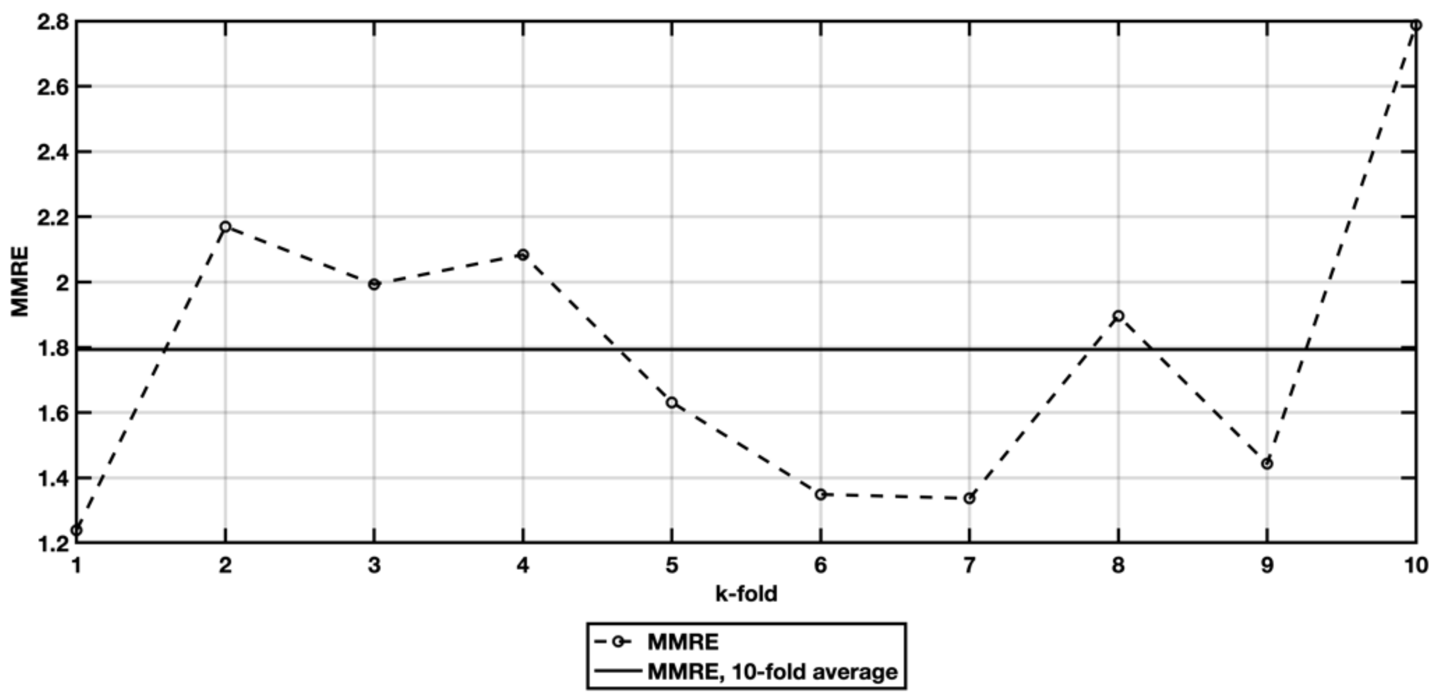
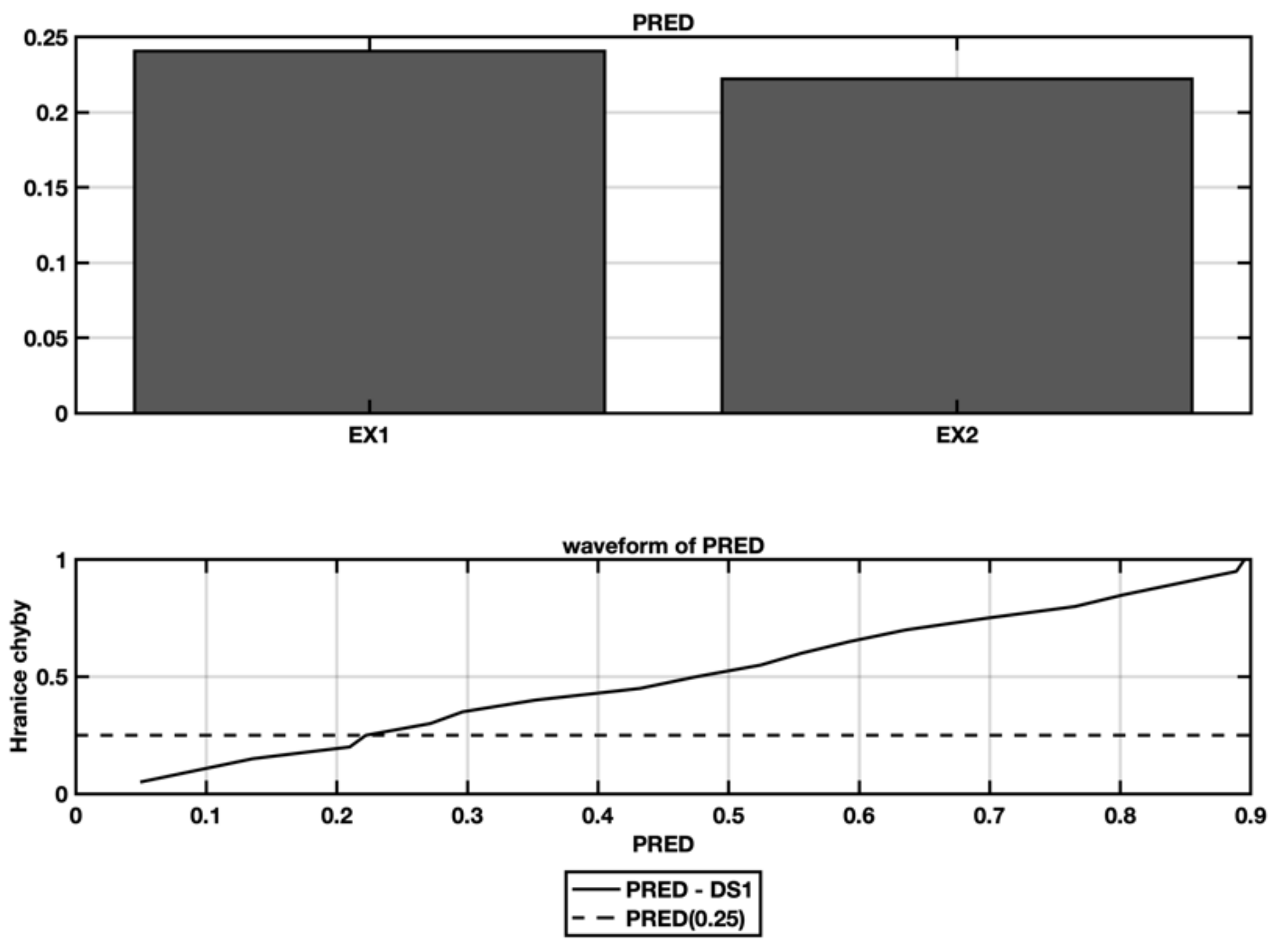
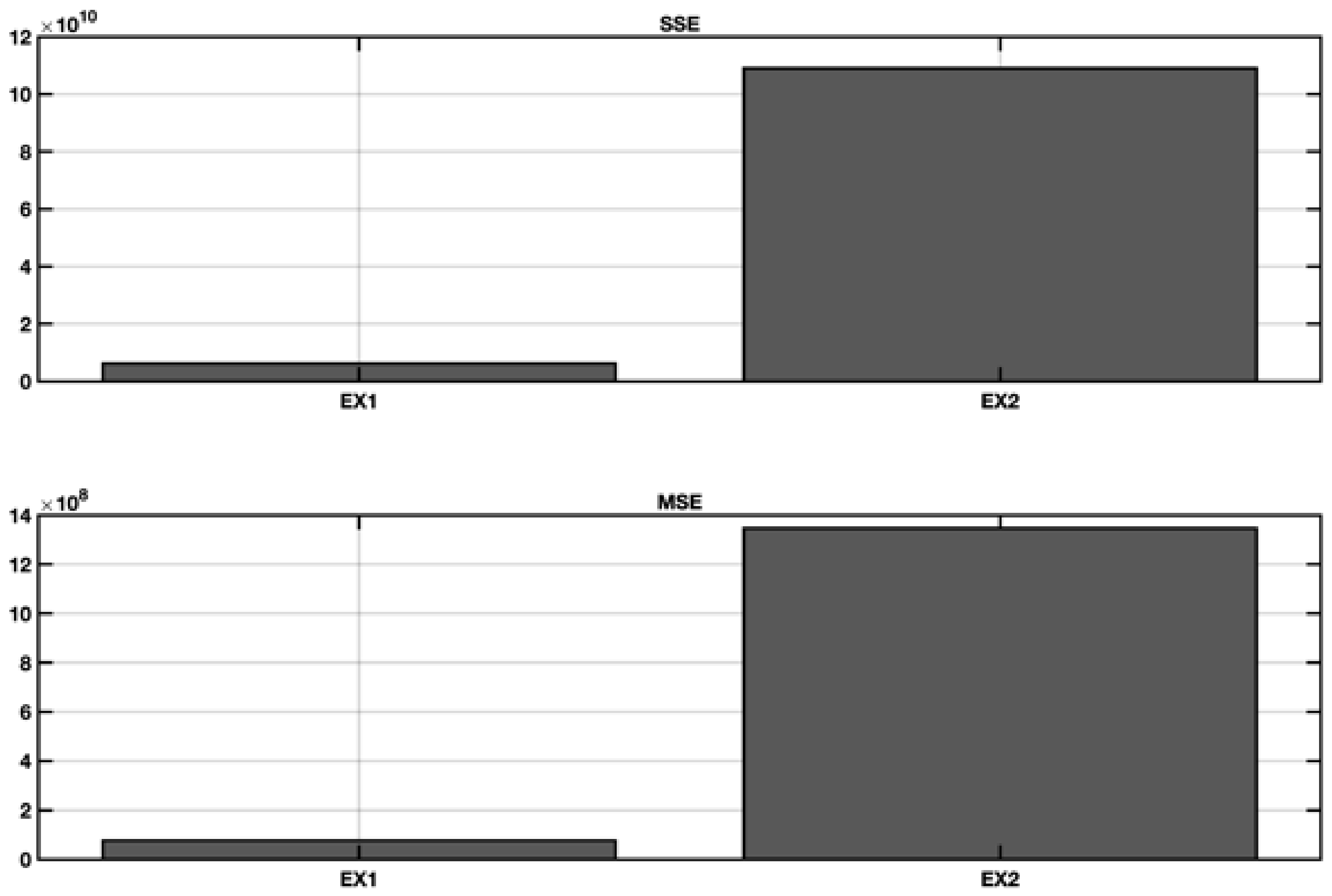
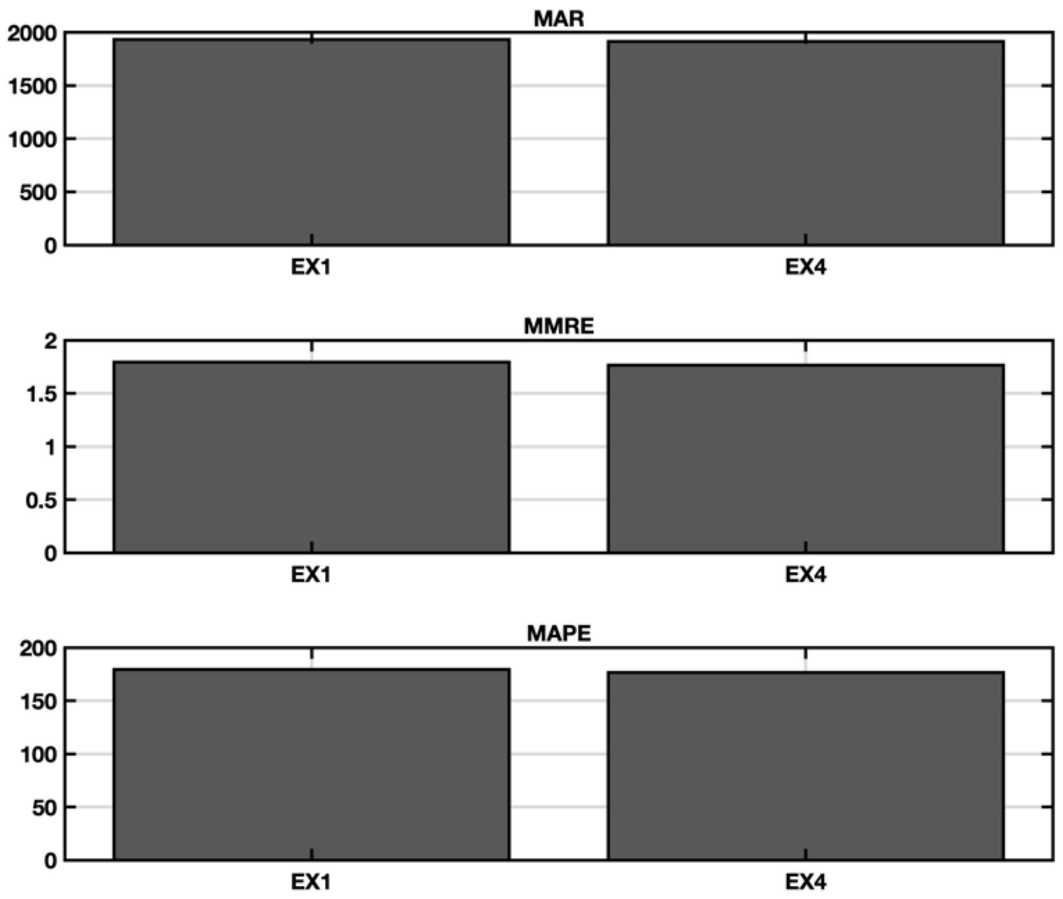
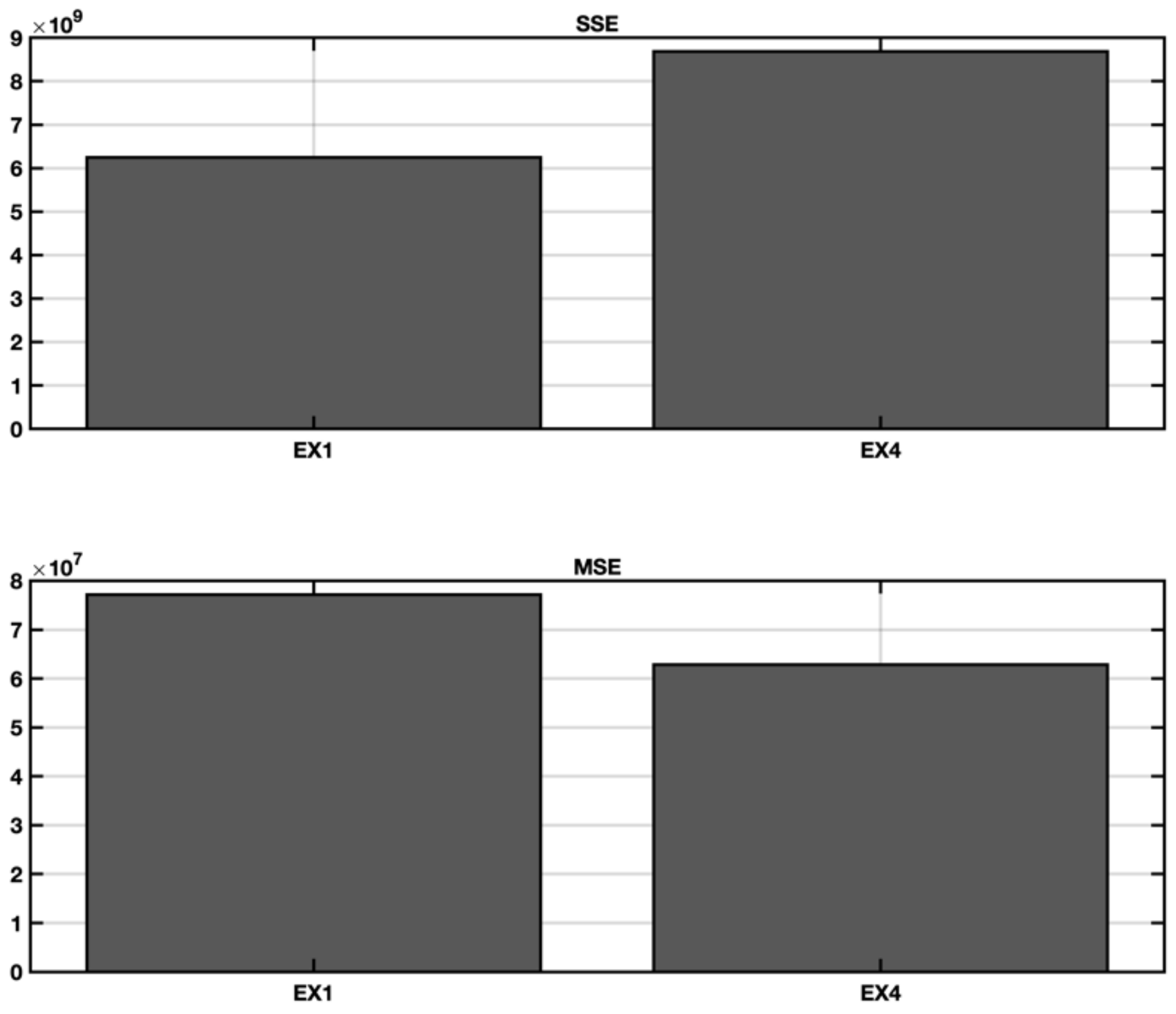
5.1. EX1—IFPUG Base Model

The IFPUG in combination with the average PDR was used as a reference method in simulations—EX1. The average PDR was determined using the IS variable [8,9] for comparison experiments.

The value of PRED (0.25) shows that the behavior within 10 test selections is balanced (Figure 3). The graph shows that 19% of the projects are estimated with an error less than 25%.

Figure 4 shows the development of the PRED value when the boundary error $l$ was changed from 0.05 to 1. From the waveform, the growth of the PRED value is almost linear. The IFPUG method is able to estimate more than 60% of projects with an error of less than 50% if the PDR based on IS variables is used. It has been reported that the accuracy of the estimation methods is 75% of the estimated projects with an error of less than 25% [44].

The other indicators (MAR, MMRE, SSE, MSE, and MAPE) show that the IFPUG method has a large EE. EEs have relatively high variability across test selections. For comparison with other methods, the average values will be used (marked as solid lines in the graphs). The MAR value (Figure 5) and the MMRE value (Figure 6) show large differences between selections, suggesting a poor/low estimation consistency. The reason is in the basic principle of estimation. When we estimate the effort, the final conversion between the project size (expressed in adjusted function points) and the effort in man-hours has a great influence.

The SSE and its mean value confirmed this conclusion. The average SSE is $3.35\times {10}^{10}$ (Figure 7). From this, the results of the IFPUG method are not sufficiently accurate for the estimating efforts.

When evaluating the MAPE (Figure 8), the mean percentage of the relative error is high. The average achieved value is 179.

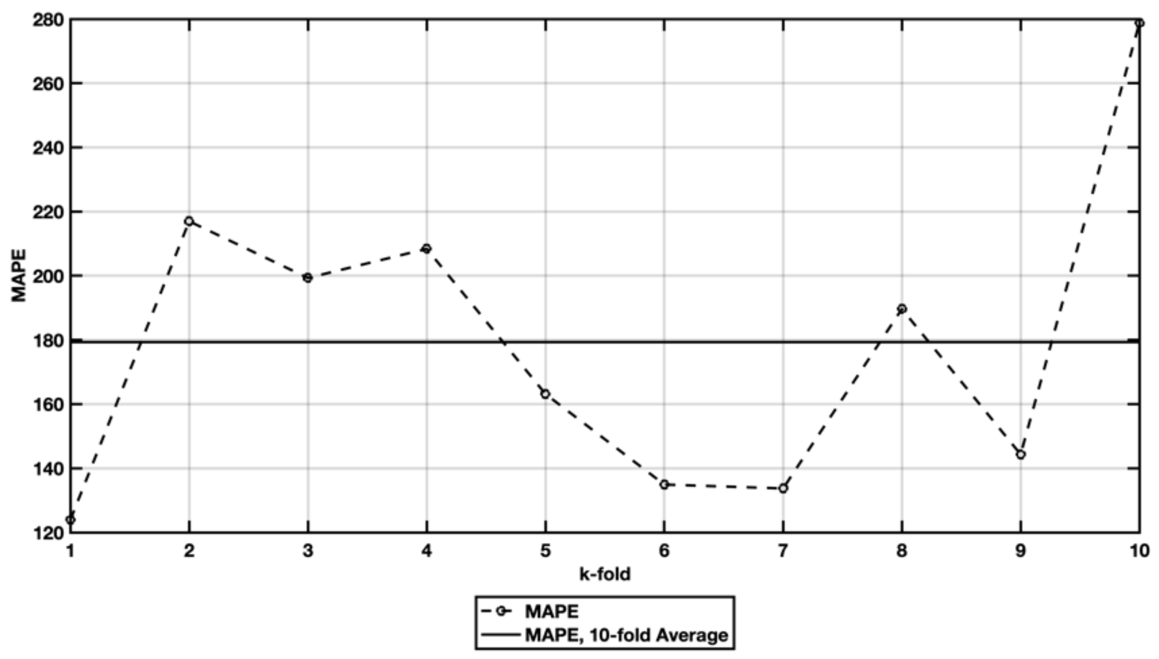
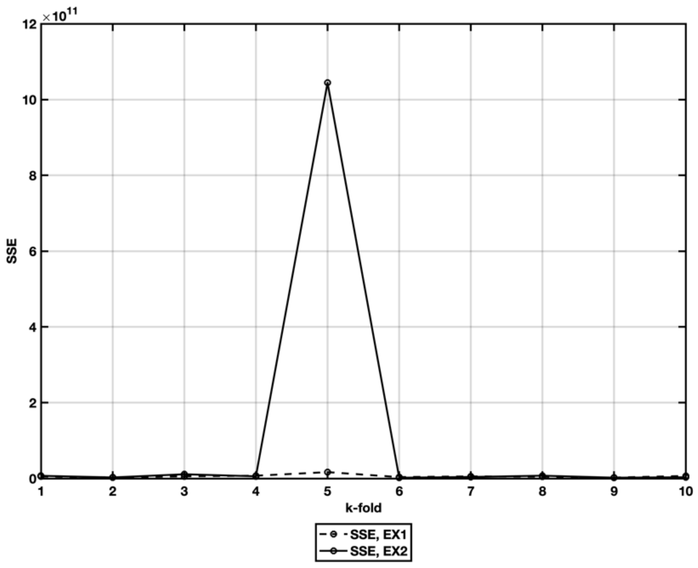
5.2. EX2—Stepwise Regresion

The results show that SR can reach a model that could be overcome by estimating EX1. A comparison between the EX1 method and the SR is displayed on the graphs of the individual criteria. Both models return an almost identical value for the PRED value (0.25). The development of the PRED value in the stepwise regression is almost linear (Figure 9). However, the MAR value is smaller for SR, similar to MAPE, which is an improvement of almost 20% compared to the EX1 method (Figure 10).

The last two criteria, SSE and MSE, show that SR (Figure 11) achieves significantly worse predictions than the EX1 method. It is evident that multiple deteriorations occur. To explain the behavior of SR, we must closely examine the SSE values in each test sample. Figure 12 shows that the overall results are significantly influenced by the poor predictive capability for five test selections. Due to the magnitude of the higher prediction errors of the five test selections compared with that of the remaining nine selections, it cannot be concluded that SR is not capable of prediction. In this case, its behavior is heavily influenced by random selection.

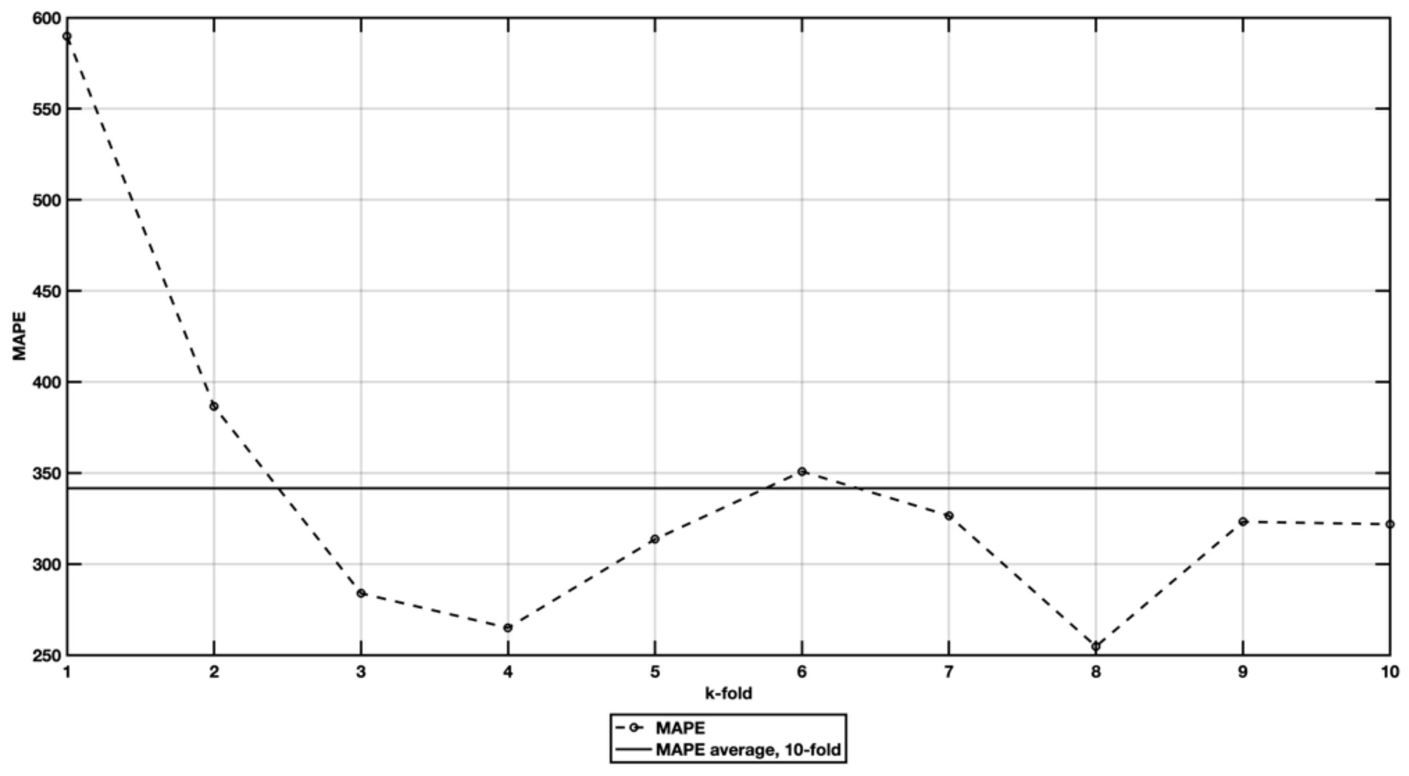
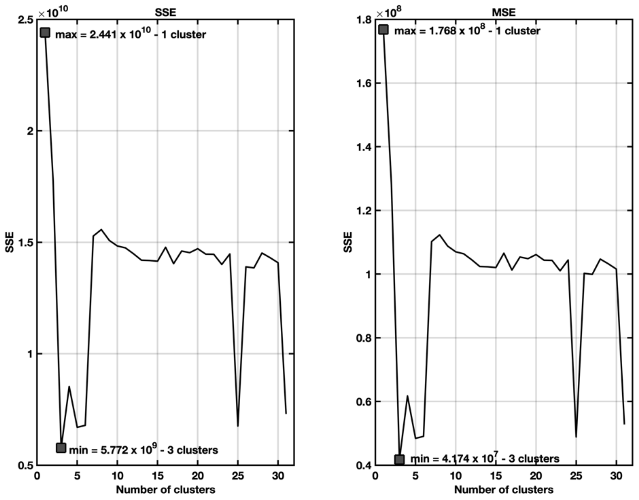
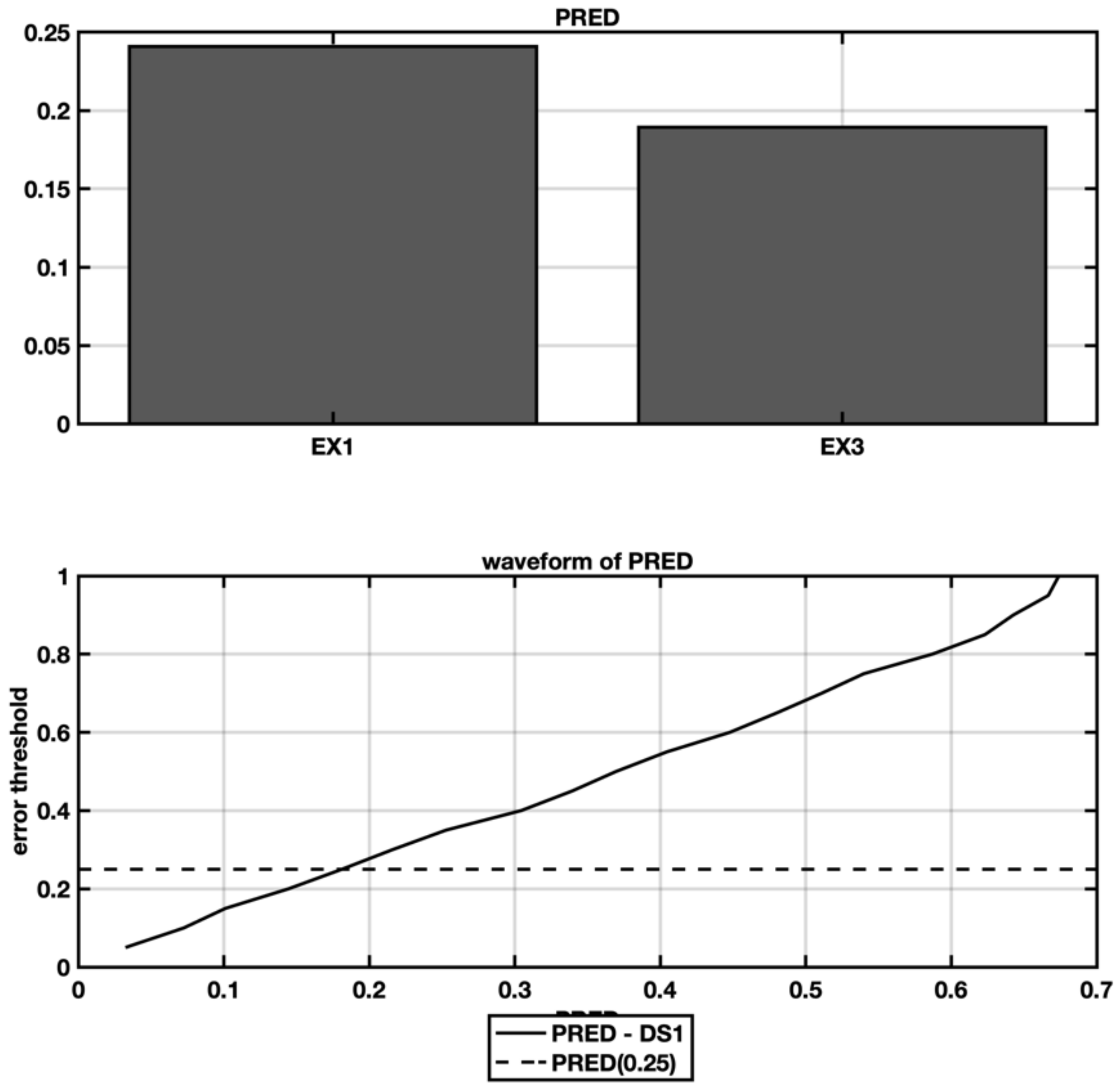
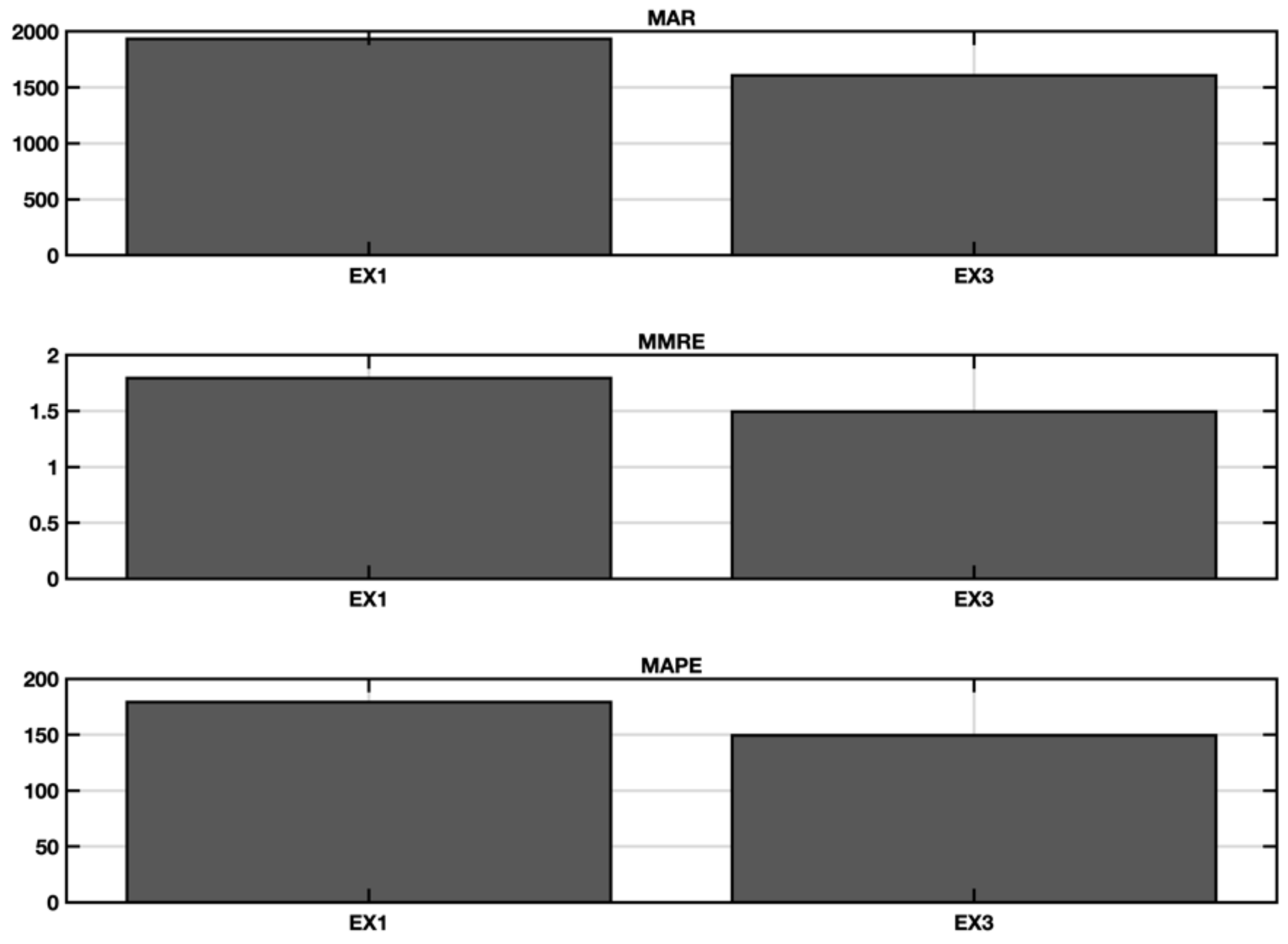
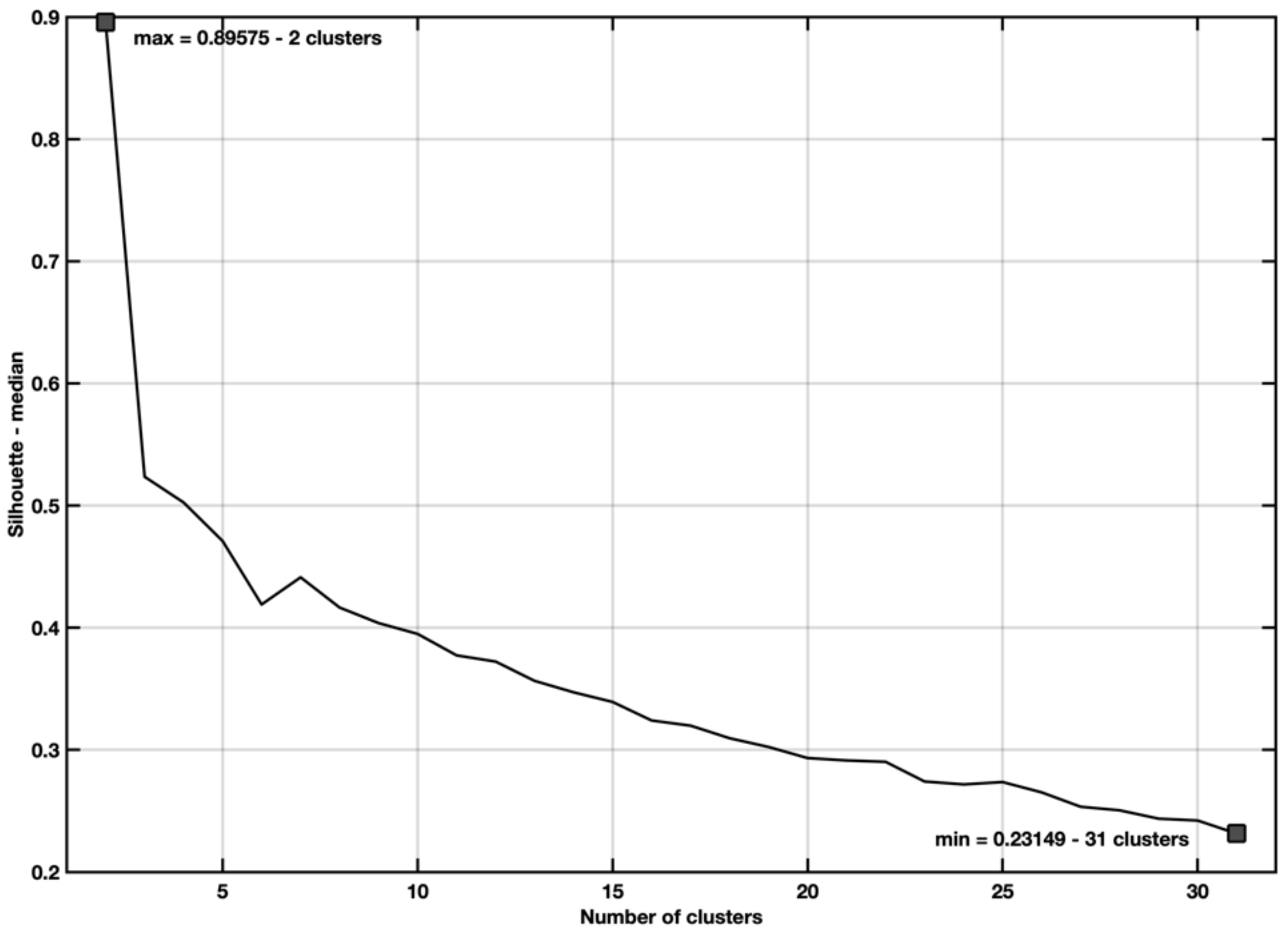
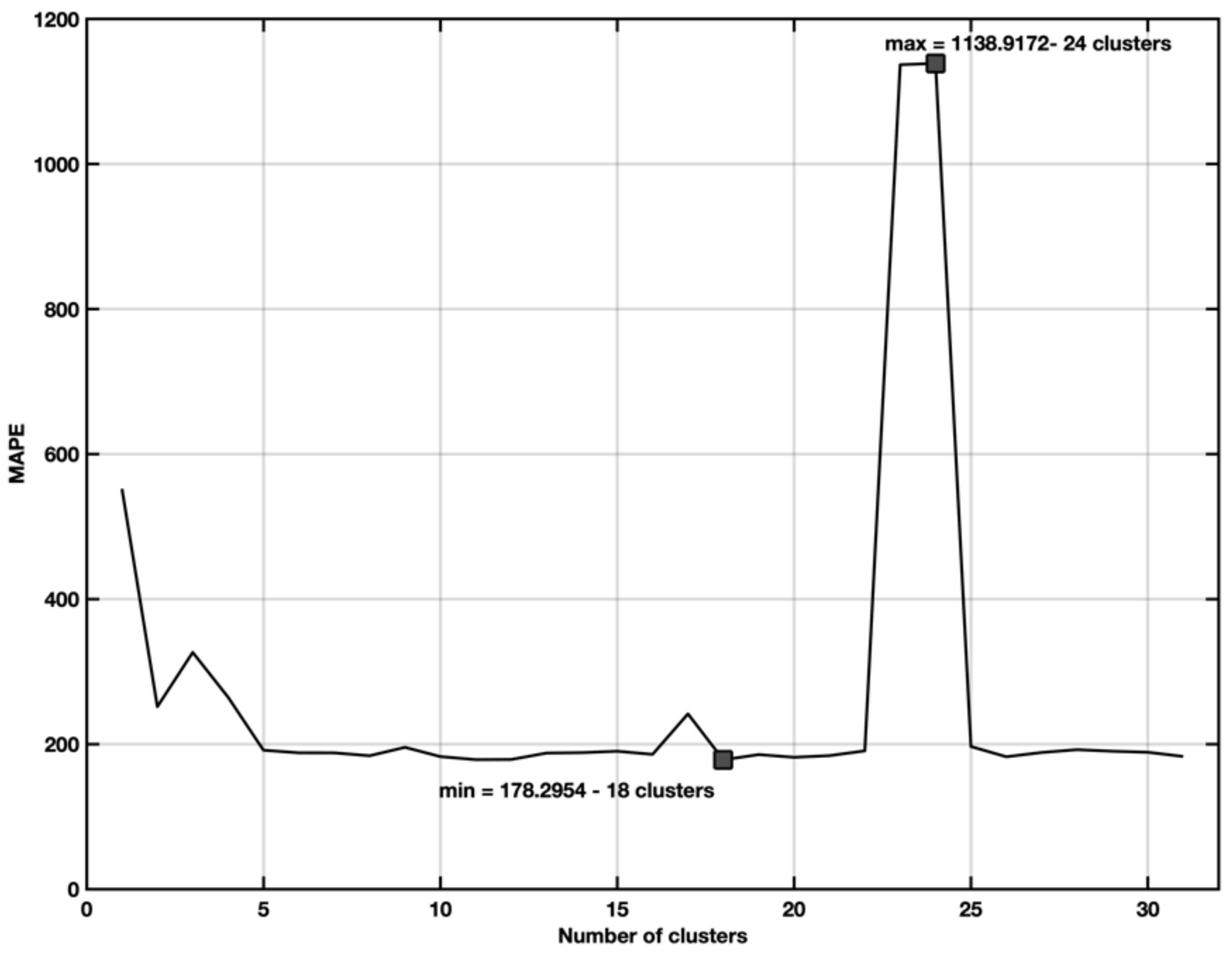
5.3. EX3—Stepwise Regression with Spectral Cluster Clustering

Figure 13 shows the graph of the waveform of the silhouette value (13). The chart shows that the projects are best classified when two clusters are used. Acceptable values are achieved for four clusters. From 5 to 31 clusters (the tested maximum), the projects are poorly classified. If the evaluation criteria applicable to the assessment of the estimate quality are considered, then better solutions exist than when only two clusters are considered.

When comparing the SR without and with clustering using a different number of clusters, the clustering has a positive effect on the improvement of the estimating efforts. Figure 14 shows a comparison of the SSE and MSE for the tested number of clusters. Clustering contributes to reductions in both the SSE and MSE of more than 34%. The graph shows the minimum value achieved for a solution with three clusters.

When the MAPE is used, the best solution is based on six clusters (Figure 15). The MAPE is 41% lower than the variant without clustering. According to the last criterion, PRED (0.25), the best option is to use three clusters. However, as apparent from Figure 16, the solution of a different number of clusters achieves similar values of PRED (0.25).

Figure 17, Figure 18 and Figure 19 are compared to EX1 (IFPUG). The PRED (0.25) shows higher accuracy for the reference method, but the other criteria indicate a higher accuracy for estimating the development effort after SC is applied.

Although the SSE does not show a significant difference between the reference method and the spectral cluster, the criteria for the MSE can be considered more favorable. A smaller MSE value indicates a smaller margin of EEs, which allows the consideration of SC with three clusters per method, which is more usable in practice.

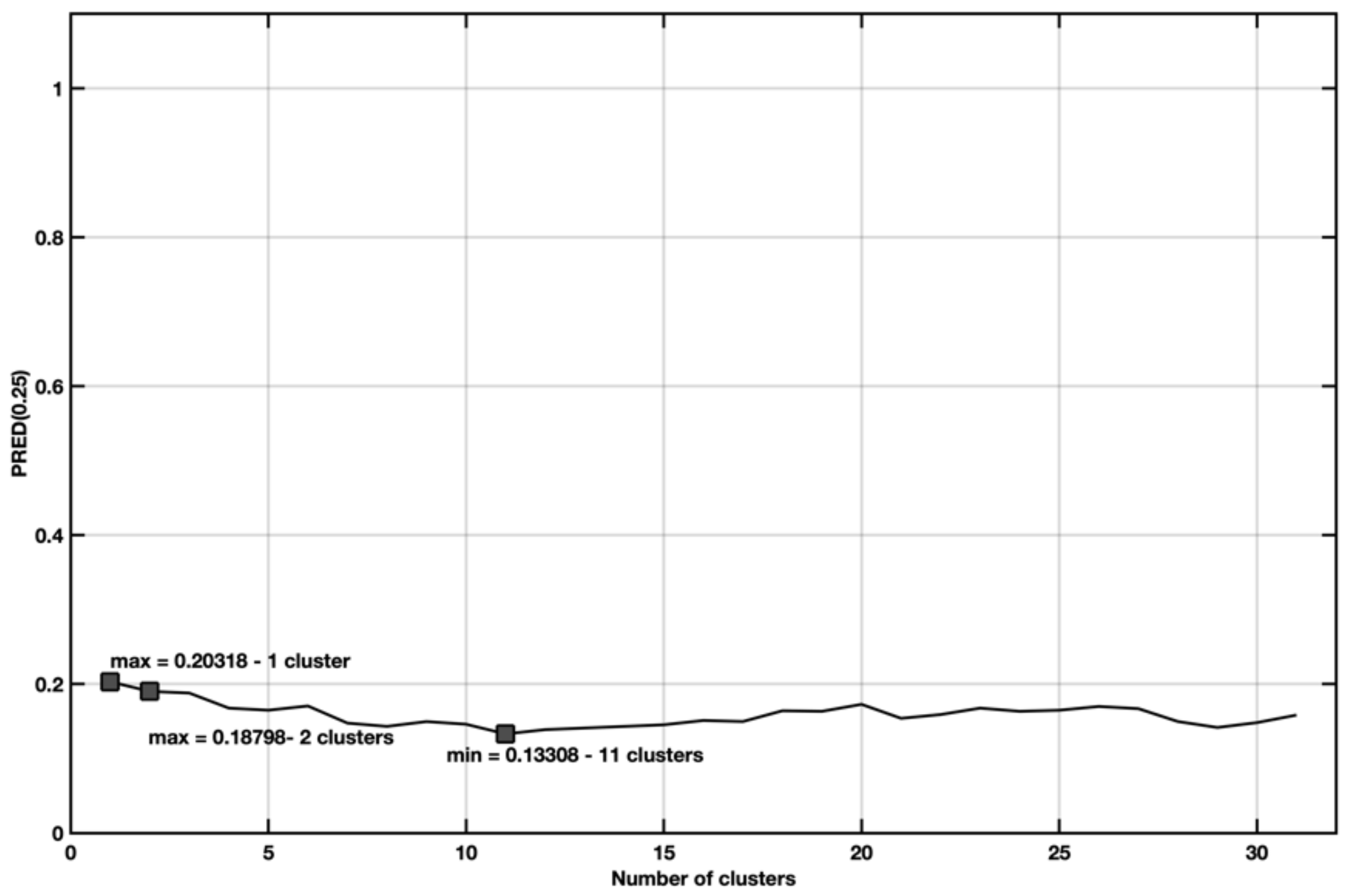
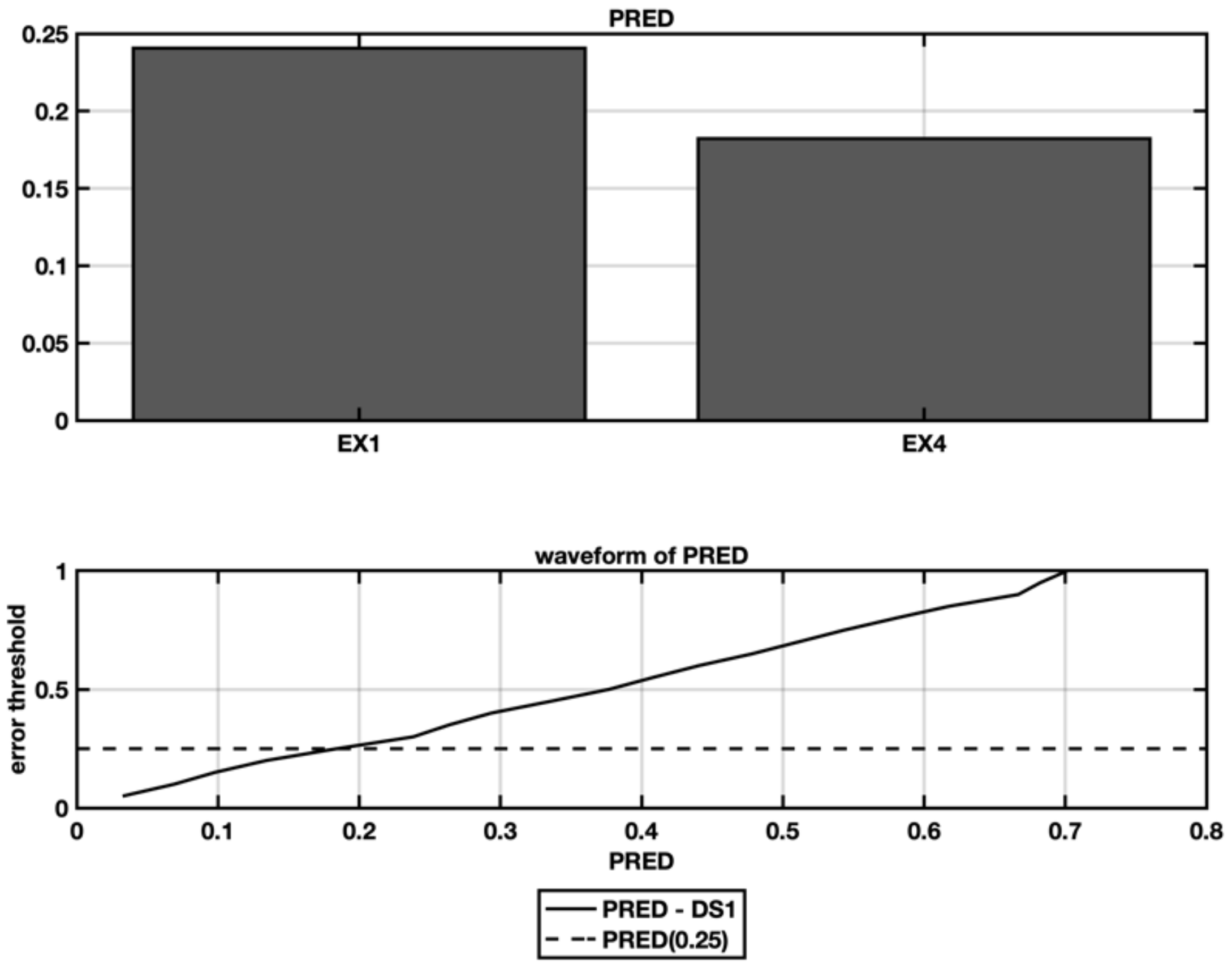
5.4. Ex4—Stepwise Regression with Spectral Clustering and Categorical Variables

Figure 20 shows a comparison of the SSE development. The best result is achieved for 29 clusters, which is contrasted with the value of the silhouette, which recommends using the solution for a maximum of five clusters and considers two clusters optimal. For the two clusters, the value of SSE is 29% worse than that for the 29 clusters.

Another reference criterion is the MAPE (Figure 21). According to this criterion, the best solution is for 11 clusters, and the worst solution is possible for 23 clusters. The unsuitability of the solution for 23 clusters is confirmed by the previous SSE criterion. For two clusters, the MAPE is 251%, which means that there has been an improvement against the variant without clustering (515%). The deterioration for the best option (11 clusters) is approximately 30%.

Compared to the PRED (0.25) parameter, it is evident (Figure 22) that the solution without clustering achieves an approximately 8% better ability to estimate with an error of less than 25% compared with the best-clustered solution (three clusters).

The SC method will be graphically compared using categorical variables (11 clusters) with the reference method (IFPUG, FP with a productivity factor). The comparison is done in Figure 23, Figure 24 and Figure 25. The reference method shows higher accuracy according to the PRED (0.25). This is also confirmed by other criteria (MAR, MMRE, and MAPE).

Considering the SSE and MSE criteria, the reference method is still more appropriate. Only the MSE shows a lower variability of EEs in SC using categorical variables. Overall, categorical variables deteriorate the estimation accuracy and cannot be recommended as clustering parameters.

6. Conclusions

In this study, experiments to evaluate SR and SC methods for IFPUG-based effort estimation are presented. Two evaluation criteria, namely, the MAPE and PRED (0.25), are chosen for the overall assessment and recommendation, which are most indicative of the practical quality of the estimate and are measurable and interpretable in industry.

Estimation models were designed based on stepwise regression models, which were compared to the IFPUG reference method. A comparison of the methods is captured in

Table 3. Comparing the best performing configuration in EX1–EX4.

Method	MAPE	PRED (0.25)
EX1	179	0.24
EX2	159	0.24
EX3—3 clusters	134	0.21
EX4—11 clusters	178	0.17

. The results show that, for the dataset, the most advantageous variant is a combination of SR and SC for three clusters.

Overall, the results show that the error for the selected variations (Table 3) is lower than that of the reference method (EX1). Regarding the first research question (RQ1), the stepwise regression method results in an improvement in the estimation assessed by the MAPE criterion by 20%. In the case of a stepwise regression variant with SC (RQ2), the MAPE criterion is reduced by 45% compared to EX1 and 25% when compared to EX2. The combination with categorical variables (RQ3) does not produce the desired improvement (when MAPE is used).

The results show that the methods based on SC and stepwise regression provide the most accurate estimates. For this reason, SC can be clearly recommended as a suitable method for preparing data for future estimation and then for each of the clusters to create an estimation model using stepwise regression.

In future research, a method of increasing accuracy will be evaluated. Models trained on clustered data or segmented data [24] show a tendency to estimate a new project more accurately.

References

- Trendowicz, A.; Jeffery, R. Software Project Effort Estimation: Foundations and Best Practice Guidelines for Success; Springer: Cham, Switzerland, 2014; 469p. [Google Scholar]
- Silhavy, P. A Software Project Effort Estimation by Using Functional Points. Habilitation Thesis, Mendel University, Brno, Czech Republic, 2019. [Google Scholar]
- McConnell, S. Software Estimation: Demystifying the Black Art; Microsoft Press: Redmond, WA, USA, 2006; 308p. [Google Scholar]
- Bundschuh, M.; Dekkers, C. The IT Measurement Compendium: Estimating and Benchmarking Success with Functional Size Measurement; Springer: Berlin, Germany, 2008; 643p. [Google Scholar]
- ISO/IEC. ISO/IEC 14143-1:2007. Information Technology-Software Measurement-Functional Size Measurement—Part 1: Definition of Concepts; ISO/IEC: Washington, DC, USA, 2007. [Google Scholar]
- Borandag, E.; Yucalar, F.; Erdogan, S.Z. A case study for the software size estimation through MK II FPA and FP methods. Int. J. Comput. Appl. Technol. 2016, 53, 309–314. [Google Scholar] [CrossRef]
- Bardsiri, V.K.; Jawawi, D.N.A.; Hashim, S.Z.M.; Khatibi, E. Increasing the accuracy of software development effort estimation using projects clustering. IET Softw. 2012, 6, 461–473. [Google Scholar] [CrossRef]
- Amazal, F.A.; Idri, A. Estimating software development effort using fuzzy clustering-based analogy. J. Softw. Evol. Process 2021, 33, e2324. [Google Scholar] [CrossRef]
- Idri, A.; Amazal, F.A.; Abran, A. Analogy-based software development effort estimation: A systematic mapping and review. Inf. Softw. Technol. 2015, 58, 206–230. [Google Scholar] [CrossRef]
- Nassif, A.; Azzeh, M.; Capretz, L.; Ho, D. Neural network models for software development effort estimation: A comparative study. Neural Comput. Appl. 2015, 28, 2369–2381. [Google Scholar] [CrossRef] [Green Version]
- Rankovic, N.; Rankovic, D.; Ivanovic, M.; Lazic, L. Improved effort and cost estimation model using artificial neural networks and taguchi method with different activation functions. Entropy 2021, 23, 854. [Google Scholar] [CrossRef] [PubMed]
- Azzeh, M.; Nassif, A.B. A hybrid model for estimating software project effort from use case points. Appl. Soft Comput. 2016, 49, 981–989. [Google Scholar] [CrossRef] [Green Version]
- Gallego, J.J.C.; Rodríguez, D.; Sicilia, M.A.; Rubio, M.G.; Crespo, A.G. Software project effort estimation based on multiple parametric models generated through data clustering. J. Comput. Sci. Technol. 2007, 22, 371–378. [Google Scholar] [CrossRef]
- Garre, M.; Cuadrado, J.J.; Sicilia, M.A.; Charro, M.; Rodríguez, D. Segmented parametric software estimation models: Using the EM algorithm with the ISBSG 8 database. In Proceedings of the 27th International Conference on Information Technology Interfaces 2005, Cavtat, Croatia, 20–23 June 2005; pp. 193–199. [Google Scholar]
- Dempster, A.P.; Laird, N.M.; Rubin, D.B. Maximum likelihood from incomplete data via the EM algorithm. J. R. Statist. Soc. Ser. B (Methodol.) 1977, 39, 1–22. [Google Scholar] [CrossRef]
- Hihn, J.; Juster, L.; Johnson, J.; Menzies, T.; Michael, G. Improving and expanding NASA software cost estimation methods. In Proceedings of the 2016 IEEE Aerospace Conference, Big Sky, MT, USA, 3–12 March 2016; pp. 1–12. [Google Scholar]
- Khatibi Bardsiri, V.; Jawawi, D.N.A.; Hashim, S.Z.M.; Khatibi, E. A flexible method to estimate the software development effort based on the classification of projects and localization of comparisons. Empir. Softw. Eng. 2014, 19, 857–884. [Google Scholar] [CrossRef]
- Kennedy, J.; Eberhart, R. Particle swarm optimization. In Proceedings of the ICNN′95—International Conference on Neural Networks, Perth, WA, Austrilia, 27 November–1 December 1995; pp. 1942–1948. [Google Scholar]
- Prokopova, Z.; Silhavy, R.; Silhavy, P. The effects of clustering to software size estimation for the use case points methods. In Software Engineering Trends and Techniques in Intelligent Systems; Silhavy, R., Silhavy, P., Prokopova, Z., Senkerik, R., Kominkova Oplatkova, Z., Eds.; Springer International Publishing: Cham, Switzerland, 2017; pp. 479–490. [Google Scholar]
- Lokan, C.; Mendes, E. Applying moving windows to software effort estimation. In Proceedings of the 2009 3rd International Symposium on Empirical Software Engineering and Measurement, Lake Buena Vista, FL, USA, 15–16 October 2009; pp. 111–122. [Google Scholar]
- Amasaki, S.; Lokan, C. The effect of moving windows on software effort estimation: Comparative study with CART. In Proceedings of the 2014 6th International Workshop on Empirical Software Engineering in Practice, Osaka, Japan, 12–13 November 2014; pp. 1–6. [Google Scholar]
- Silhavy, R.; Silhavy, P.; Prokopova, Z. Evaluating subset selection methods for use case points estimation. Inf. Softw. Technol. 2018, 97, 1–9. [Google Scholar] [CrossRef]
- Minku, L.L. A novel online supervised hyperparameter tuning procedure applied to cross-company software effort estimation. Empir. Softw. Eng. 2019, 24, 3153–3204. [Google Scholar] [CrossRef] [Green Version]
- Silhavy, P.; Silhavy, R.; Prokopova, Z. Categorical variable segmentation model for software development effort estimation. IEEE Access 2019, 7, 9618–9626. [Google Scholar] [CrossRef]
- Ventura-Molina, E.; López-Martín, C.; López-Yáñez, I.; Yáñez-Márquez, C. A novel data analytics method for predicting the delivery speed of software enhancement projects. Mathematics 2020, 8, 2002. [Google Scholar] [CrossRef]
- International Function Point Users Group (IFPUG). Available online: https://www.ifpug.org (accessed on 16 January 2021).
- ISBSG. ISBSG Development & Enhancement Repository-Release 13. Available online: http://isbsg.org (accessed on 2 February 2015).
- Ezghari, S.; Zahi, A. Uncertainty management in software effort estimation using a consistent fuzzy analogy-based method. Appl. Soft Comput. 2018, 67, 540–557. [Google Scholar] [CrossRef]
- Sarro, F.; Petrozziello, A. Linear programming as a baseline for software effort estimation. ACM Trans. Softw. Eng. Methodol. 2018, 27, 1–28. [Google Scholar] [CrossRef]
- Azzeh, M.; Nassif, A.B.; Banitaan, S. Comparative analysis of soft computing techniques for predicting software effort based use case points. IET Softw. 2018, 12, 19–29. [Google Scholar] [CrossRef]
- Azzeh, M.; Nassif, A.B. Analyzing the relationship between project productivity and environment factors in the use case points method. J. Softw. Evol. Process 2017, 29, e1882. [Google Scholar] [CrossRef] [Green Version]
- Silhavy, R.; Silhavy, P.; Prokopova, Z. Analysis and selection of a regression model for the use case points method using a stepwise approach. J. Syst. Softw. 2017, 125, 1–14. [Google Scholar] [CrossRef] [Green Version]
- Silhavy, P.; Silhavy, R.; Prokopova, Z. Evaluation of data clustering for stepwise linear regression on use case points estimation. In Software Engineering Trends and Techniques in Intelligent Systems; Silhavy, R., Silhavy, P., Prokopova, Z., Senkerik, R., Kominkova Oplatkova, Z., Eds.; Springer International Publishing: Cham, Switzerland, 2017; pp. 491–496. [Google Scholar]
- Von Luxburg, U. A tutorial on spectral clustering. Stat. Comput. 2007, 17, 395–416. [Google Scholar] [CrossRef]
- Silhavy, R.; Silhavy, P.; Prokopova, Z. Improving algorithmic optimisation method by spectral clustering. In Software Engineering Trends and Techniques in Intelligent Systems, Proceedings of the Computer Science On-line Conference, Prague, Czech Republic, 26–29 April 2017; Springer: Cham, Switzerland, 2017; pp. 1–10. [Google Scholar]
- Soltanolkotabi, M.; Elhamifar, E.; Candes, E.J. Robust subspace clustering. Ann. Stat. 2014, 42, 669–699. [Google Scholar] [CrossRef] [Green Version]
- Urbanek, T.; Prokopova, Z.; Silhavy, R.; Vesela, V. Prediction accuracy measurements as a fitness function for software effort estimation. SpringerPlus 2015, 4, 778. [Google Scholar] [CrossRef] [PubMed] [Green Version]
- Shepperd, M.; MacDonell, S. Evaluating prediction systems in software project estimation. Inf. Softw. Technol. 2012, 54, 820–827. [Google Scholar] [CrossRef] [Green Version]
- Idri, A.; Abnane, I.; Abran, A. Evaluating Pred(p) and standardized accuracy criteria in software development effort estimation. J. Softw. Evol. Process 2018, 30, e1925. [Google Scholar] [CrossRef]
- De Myttenaere, A.; Golden, B.; Le Grand, B.; Rossi, F. Mean absolute percentage error for regression models. Neurocomputing 2016, 192, 38–48. [Google Scholar] [CrossRef] [Green Version]
- Silhavy, P.; Silhavy, R.; Prokopova, Z. Stepwise regression clustering method in function points estimation. In Computational and Statistical Methods in Intelligent Systems, Proceedings of the Computational Methods in Systems and Software, Szczecin, Poland, 12–14 September 2018; Springer: Cham, Switzerland, 2018; pp. 333–340. [Google Scholar]
- Jajuga, K.; Sokolowski, A.; Bock, H.H. Classification, Clustering, and Data Analysis: Recent Advances and Applications; Springer Science & Business Media: Berlin, Germany, 2012. [Google Scholar]
- Fraley, C.; Raftery, A. How many clusters? Which clustering method? Answers via model-based cluster analysis. Comput. J. 1998, 41, 578–588. [Google Scholar] [CrossRef]
- Conte, S.; Dunsmore, H.; Shen, Y. Software Engineering Metrics and Models; Benjamin-Cummings Publishing: Redwood City, CA, USA, 1986. [Google Scholar]