Abstract
In previous work, it was shown that if certain series based on sums over primes of non-principal Dirichlet characters have a conjectured random walk behavior, then the Euler product formula for its L-function is valid to the right of the critical line , and the Riemann hypothesis for this class of L-functions follows. Building on this work, here we propose how to extend this line of reasoning to the Riemann zeta function and other principal Dirichlet L-functions. We apply these results to the study of the argument of the zeta function. In another application, we define and study a one-point correlation function of the Riemann zeros, which leads to the construction of a probabilistic model for them. Based on these results we describe a new algorithm for computing very high Riemann zeros, and we calculate the googol-th zero, namely -th zero to over 100 digits, far beyond what is currently known. Of course, use is made of the symmetry of the zeta function about the critical line.
1. Introduction
There are many generalizations of Riemann’s zeta function to other Dirichlet series, which are also believed to satisfy a Riemann hypothesis. A common opinion, based largely on counterexamples, is that the L-functions for which the Riemann hypothesis is true enjoy both an Euler product formula and a functional equation. However, a direct connection between these properties and the Riemann hypothesis has not been formulated in a precise manner. In [1,2] a concrete proposal making such a connection was presented for Dirichlet L-functions, and those based on cusp forms, due to the validity of the Euler product formula to the right of the critical line. In contrast to the non-principal case, in this approach the case of principal Dirichlet L-functions, of which Riemann zeta is the simplest, turned out to be more delicate, and consequently it was more difficult to state precise results. In the present work, we attempt to further address this special case, although as we will explain, the results are not as conclusive as for the non-principal case. What is new that we present here a different way to understand the extent in which the truncated Euler product is a good approximation. We then use this to approximate the argument of the zeta function on the critical line. We also study one-point statistics of the Riemann zeros, in contrast to the two-point correlation functions that are widely studied.
Let be a Dirichlet character modulo k and its L-function with . It satisfies the Euler product formula
where is the n-th prime. The above formula is valid for , since both sides converge absolutely. The important distinction between principal verses non-principal characters is the following. For non-principal characters, the L-function has no pole at ; thus, there exists the possibility that the Euler product is valid partway inside the strip, i.e., has abscissa of convergence . It was proposed in [1,2] that for this case. In contrast, now consider L-functions based on principal characters. The latter character is defined as if n is coprime to k and zero otherwise. The Riemann zeta function is the trivial principal character of modulus with all . L-functions based on principal characters do have a pole at , and therefore have abscissa of convergence , which implies the Euler product in the form given above strictly cannot be valid inside the critical strip . Nevertheless, in this paper we will show how a truncated version of the Euler product formula can be approximately valid for .
The primary aim of the work [1,2] was to determine what specific properties of the prime numbers would imply that the Riemann hypothesis is true. This is the opposite of the more well-studied question of what the validity of the Riemann hypothesis implies for the fluctuations in the distribution of primes. The answer proposed was simply based on the multiplicative independence of the primes, which to a large extent underlies their pseudo-random behavior. To be more specific, let for . In [1,2] it was proven that if the series
is , then the Euler product converges for and the Formula (1) is valid to the right of the critical line. In fact, we only need up to logs (see Remark 1); when we write , it is implicit that this can be relaxed with logarithmic factors. For non-principal characters, the allowed angles are equally spaced on the unit circle, and it was conjectured in [2] that the above series with behaves like a random walk due to the multiplicative independence of the primes, and this is the origin of the growth. Furthermore, this result extends to all t since domains of convergence of Dirichlet series are always half-planes. Taking the logarithm of (1), one sees that is never infinite to the right of the critical line and thus has no zeros there. This, combined with the functional equation that relates to , implies there are also no zeros to the left of the critical line, so that all zeros are on the line. The same reasoning applies to cusp forms if one also uses a non-trivial result of Deligne [2].
In this article, we reconsider the principal Dirichlet case, specializing to Riemann zeta itself, since identical arguments apply to all other principal cases with . In much more recent work, a different approach to the non-principal case was studied based on Möbius inversion [3]. Here all angles , so one needs to consider the series
which now strongly depends on t. On the one hand, the case of principal Dirichlet L-functions is complicated by the existence of the pole, and, as we will see, one consequently needs to truncate the Euler product to make sense of it. On the other hand, can be estimated using the prime number theorem since it does not involve sums over non-trivial characters , and this aids the analysis. This is in contrast to the non-principal case, where, however well-motivated, we had to conjecture the random walk behavior alluded to the above, so in this respect the principal case is potentially simpler. To this end, a theorem of Kac (Theorem 1 below) nearly does the job: in the limit , which is also a consequence of the multiplicative independence of the primes. This suggests that one can also make sense of the Euler product formula in the limit . However this is not enough for our main purpose, which is to have a similar result for finite t which we will develop.
This article is mainly based on our previous work [1,2] but provides a more detailed analysis and extends it in several ways. It was suggested in [1] that one should truncate the series at an N that depends on t. First, in the next section we explain how a simple group structure underlies a finite Euler product, which relates it to a generalized Dirichlet series which is a subseries of the Riemann zeta function. Subsequently we estimate the error under truncation, which shows explicitly how this error is related to the pole at , as expected. The remainder of the paper, Section 4 and Section 5, presents various applications of these ideas. We use them to study the argument of the zeta function. We present an algorithm to calculate very high zeros, far beyond what is currently known. We also study the statistical fluctuations of individual zeros, in other words, a one-point correlation function.
In many respects, our work is related to the work of Gonek et al. [4,5], which also considers a truncated Euler product. The important difference is that the starting point in [4] is a hybrid version of the Euler product which involves both primes and zeros of zeta. Only after assuming the Riemann hypothesis can one explain in that approach why the truncated product over primes is a good approximation to zeta. In contrast, here we do not assume anything about the zeros of zeta, since the goal is to actually understand their location.
We are unable to provide fully rigorous proofs of some of the statements below; however, we do provide supporting calculations and numerical work. In order to be clear on this, below “Proposal” signifies the most important claims that we could not rigorously prove, and should not be taken as a “Proposition” in the usual formal mathematical sense.
2. Algebraic Structure of Finite Euler Products
The aim of this section is to define properly the objects we will be dealing with. In particular we will place finite Euler products on the same footing as other generalized Dirichlet series. The results are straightforward and are mainly definitions.
Definition 1.
Fix a positive integer N and let denote the first N primes where . From this set one can generate an abelian group of rank N with elements
where the group operation is ordinary multiplication. Clearly where are the positive rational numbers. There are an infinite number of integers in which form a subset of the natural numbers . We will denote this set as , and elements of this set simply as .
Definition 2.
Fix a positive integer N. For every integer we can define the character :
Clearly, for a prime p, if .
Definition 3.
Fix a positive integer N and let s be a complex number. Based on , we can define the infinite series
which is a generalized Dirichlet series. There are an infinite number of terms in the above series since is infinitely dimensional.
Example 1.
For instance
Because of the group structure of , satisfies a finite Euler product formula:
Proposition 1.
Let be the abscissa of convergence of the series where ; namely, converges for . Then, in this region of convergence, satisfies a finite Euler product formula:
Proof.
Based on the completely multiplicative property of the characters,
one has
The result follows, then, from the fact that if . □
Example 2.
Let , so that . Then the above Euler product formula (7) is simply the standard formula for the sum of a geometric series:
Here the abscissa of convergence is .
The series defined in (6) has some interesting properties:
- (i)
- For finite N the product is finite for , thus the infinite series converges for for any finite N.
- (ii)
- Since the logarithm of the product is finite, for finite N, has no zeros nor poles for . Thus the Riemann zeros and the pole at arise from the primes at infinity , i.e., in the limit . In this limit all integers are included in the sum (6) that defines since . This is in accordance with the fact that the pole is a consequence of there being an infinite number of primes.
The property (ii) implies that, in some sense, the Riemann zeros condense out of the primes at infinity . Formally one has
However, since N is going to infinity, the above is true only where the series formally converges as a Dirichlet series, which, as discussed in the Introduction, is . Nevertheless, for very large but finite N, the function can still be a good approximation to inside the critical strip, since for finite N there is convergence of for . This is the subject of the next section, where we show that a finite Euler product formula is valid for in a manner that we will specify.
3. Finite Euler Product Formula at Large N to the Right of the Critical Liine
In this section we propose that the Euler product formula can be a very good approximation to for and large t if N is chosen to depend on t in a specific way which was already proposed in [1,2]. The new result presented here is an estimate of the error due to the truncation.
The random walk property we will build upon is based on a central limit theorem of Kac [6], which largely follows from the multiplicative independence of the primes:
Theorem 1.
(Kac) Let u be a random variable uniformly distributed on the interval , and define the series
Then in the limit and , approaches the normal distribution , namely
where P denotes the probability for the set.
We wish to use the above theorem to conclude something about for a fixed, non-random t. Based on Theorem 1, we suggest the following for non-random, but large t: For any ,
We could not rigorously prove this statement, however we can provide a heuristic argument. As , even though u is random, the vast majority of them are tending to ∞. One then uses the normal distribution in Theorem 1. In the following we will provide indirect numerical evidence.
Remark 1.
The proof of convergence of the Euler product in [2] is not spoiled if the bound on is relaxed up to logs. For instance, if in the limit , , as suggested by the law of iterated logarithms relevant to central limit theorems, this is fine, as is for any positive power a.
A consequence of Theorem 1 and the comments following it is that the Euler product formula is valid to the right of the critical line in the limit , at least formally. Namely for ,
As shown in [1,2] and discussed in the Introduction, this formally follows from the growth of . The problem with the above formula is that due to the double limit on the RHS, it is not rigorously defined. For instance, it could depend on the order of limits. It is thus desirable to have a version of (14) where N and t are taken to infinity simultaneously. Namely, we wish to truncate the product at an that depends on t with the property that . One can then replace the double limit on the RHS of (14) with one limit , or equivalently .
There is no unique choice for , but there is an optimal upper limit, , with its integer part, which we now describe. We can use the prime number theorem to estimate :
where is the usual exponential-integral function, and we have used
The prime number theorem implies . Using this in (15) and imposing leads to .
Based on the above, henceforth we will always assume the following properties of :
and will not always display the t dependence of N. Equation (14) now formally becomes
Extensive and compelling numerical evidence supporting the above formula was already presented in [1].
Based on the above results we are now in a position to study the following important question. If we fix a finite but large t, and truncate the Euler product at , which is finite, what is the error in the approximation to to the right of the critical line? We estimate this error as follows:
Proposal 1.
Let satisfy (17). Then for and large t,
where is the actual ζ function defined by analytic continuation and
is finite (except at the pole ) and satisfies
namely the error goes to zero as .
We provide the following supporting argument, although not a rigorous proof, for this Proposal. From (18), one concludes that (19) must hold in the limit of large t with satisfying (21). The logarithm of (19) reads
First assume . Then, in the limit of large t, the error upon truncation is the part that is neglected in (18):
Expanding out the logarithm, one has
where, in the second line, we again used the prime number theorem to approximate the sum over primes. Next, using , one obtains (20). Finally, the above expression can be continued into the strip if since , which goes to zero as if . The latter also implies (21).
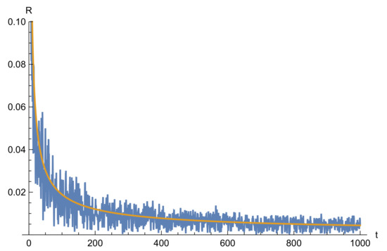
Proposal 1 makes it clear that the need for a cut-off originates from the pole at , since as long as , the error in (20) is finite. The error becomes smaller and smaller the further one is from the pole, i.e., as . In Figure 1, we numerically illustrate Proposal 1 inside the critical strip.
Remark 2.
For estimating errors at large t, the following formula is useful:
Proposal 2.
Assuming Proposal 1, all non-trivial zeros of are on the critical line.
Proof.
Taking the logarithm of the truncated Euler product, one obtains (22). If there were a zero ρ with , then . However, the right hand side of (22) is always finite; thus there are no zeros to the right of the critical line. The functional equation relating to shows there are also no zeros to the left of the critical line. □
Remark 3.
Interestingly, Proposal 1 and Theorem 2 imply that proving the validity of the Riemann hypothesis is under better control the higher one moves up the critical line. For instance, it is known that all zeros are on the line up to , and beyond this, the error is too small to spoil the validity of the Riemann hypothesis. Henceforth, we assume the RH.
4. One-Point Correlation Function of the Riemann Zeros
Montgomery conjectured that the pair correlation function of ordinates of the Riemann zeros on the critical line satisfy GUE statistics [7]. Being a two-point correlation function, it is a reasonably complicated statistic. In this section, we propose a simpler one-point correlation function that captures the statistical fluctuations of individual zeros.
Let be the exact ordinate of the n-th zero on the critical line, with and so forth. The single equation is known to have an infinite number of non-trivial solutions . In [8], by placing the zeros in one-to-one correspondence with the zeros of a cosine function, the single equation was replaced by an infinite number of equations, one for each that depends only on n:
where is the Riemann–Siegel function:
The Equation (26) involves the important function
It is important that the approaches the critical line from the right, since this is where the Euler product formula is valid in the sense described above. This equation was used to calculate zeros very accurately in [8], up to thousands of digits. There is no need for a cut-off in the above equation since the term is defined for arbitrarily high t by standard analytic continuation. One aspect of this equation is the following theorem:
Theorem 2.
(França-LeClair) If there is a unique solution to the Equation (26) for every positive integer n, then the Riemann hypothesis is true, and furthermore, all zeros are simple.
Remark 4.
Details of the proof are in [8]. The main idea is that if there is a unique solution, then the zeros are enumerated by the integer n and can be counted along the critical line, and the resulting counting formula coincides with a well-known result due to Backlund for the number of zeros in the entire critical strip. The zeros are simple because the zeros of the cosine are simple. The above theorem is another approach towards proving the Riemann hypothesis; however, it is not entirely independent of the above approach based on the Euler product formula, in particular Theorem 2. In [8], we were unable to prove there is a unique solution because we did not have sufficient control over the relevant properties of the argument of ζ on the critical line.
If the term is ignored, then there is indeed a unique solution for all n since is a monotonically increasing function of t. Using its asymptotic expansion for large t, Equation (34) below, and dropping the term, then the solution is
where W is the Lambert W-function. The only way there would fail to be a solution is if is not well defined for all t. We point out that the Lambert function was used in connection with the Riemann zeros in [9]; however, the meaning does not seem to be the same as in this article.
The fluctuations in the zeros come from since is a smooth function of n. These small fluctuations are shown in Figure 2. Let us define . One needs to properly normalize , taking into account that the spacing between zeros decreases as . To this end we expand the Equation (26) around . Using , one obtains where is the derivative with respect to t. Using , this leads us to define
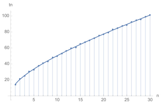
Figure 2.
The first 30 Riemann zeros . The smooth curve is the approximation in (29), whereas the dots are the actual zeros .
The probability distribution of the set
for large M is then an interesting property to study. Here “probability" is defined as the frequency of occurrence. The origin of the statistical fluctuations of is ultimately the fluctuations in the primes.
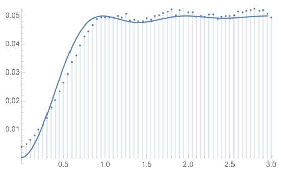
In Figure 3, we plot the distribution of for . It closely resembles a normal distribution. Let us suppose does indeed satisfy a normal distribution . Using some known properties of , together with the Equation (30), we can propose then the following. First, one expects that the average of is zero, since it is known that the average of is zero; thus . Up to the height t that we have studied, is nearly always on the principal branch, i.e., up to some reasonably high t on the order of or more. Then at each jump by 1 at , on average passes through zero. This implies that the average . For a normal distribution . Thus one expects the standard deviation of to be . In Figure 3 we present results for the first -th known exact zeros. The distribution function fits a normal distribution with rather well. Performing a fit, one finds . For higher values of M around , a fit gives , which is closer to the predicted value. We emphasize, however, that this approximate prediction for assumes is on the principal branch, which is not expected to hold for arbitrarily high t.

Figure 3.
The probability distribution for the set defined in (31) for . The smooth curve is the normal distribution with .
If we approximate the distribution of as normal, then we can construct a simple probabilistic model of the Riemann zeros:
Definition 4. A probabilistic model of the Riemann zeros.
Let be a random variable with normal distribution . Then a probabilistic model of the zeros can be defined as the set , where
and is defined in (29). In the above formula is chosen at random independently for each n.
The statistical model (32) is rather simplistic, since it is just based on a normal distribution for and is smooth and completely deterministic. A natural question then arises. Does the pair correlation function of satisfy GUE statistics as does the actual zeros ? It is certainly interesting to study the two-point correlation function of . Montgomery’s pair correlation conjecture can be stated as follows. Let denote the number of zeros up to height T, where . Let denote zeros in the range . Then in the limit of large T:
where is a normalized distance between zeros .
In Figure 4, we plot the pair correlation function for the first -th ’s. We chose , since in this range of n, this gives a better fit to the normal distribution of the one-point function. The results are reasonably close to the GUE prediction (33), especially considering that for just the first true zeros the fit to the GUE prediction is not perfect; for much higher zeros it is significantly better [10].
5. Computing Very High Zeros from the Primes
This section can be viewed as providing additional numerical evidence for some of the previous results. We will be calculating from the primes using the truncated Euler product. Since this requires , this is pushing the limit of the validity of the truncated Euler product formula; nevertheless we will obtain reasonable results. We emphasize that this method has nothing to do with the random model for the zeros in Definition 4, but rather relies on the Euler product formula to calculate .
Many very high zeros of have been computed numerically, beginning with the work of Odlyzko. All zeros up to the -th have been computed and are all on the critical line [11]. Beyond this, the computation of zeros remains a challenging open problem. However, some zeros around the -st and -nd are known [12]. In this section we describe a new and simple algorithm for computing very high zeros based on the above reasoning. It will allow us to go much higher than the known zeros since it does not require numerical implementation of the function itself, but rather only requires knowledge of some of the lower primes.
Let us first discuss the numerical challenges involved in computing high zeros from the Equation (26) based on the standard Mathematica package. The main difficulty is that one needs to implement the term. Mathematica computes , i.e., on the principal branch, however near a zero this is likely to be valid based on the discussion in Section 4. The main problem is that Mathematica can only compute for t below some maximum value around . This was sufficient to calculate up to the -th zero from (26) in [8]. The term must also be implemented to very high t, which is also limited in Mathematica.
We deal with these difficulties first by computing from the Euler product formula involving a finite sum over primes. Then, the term can be accurately computed using corrections to Stirling’s formula:
Let denote the ordinate of the n-th zero computed using the first N primes based on (26). For high zeros, it is approximately the solution to the following equation
where it is implicit that . The important property of this equation is that it no longer makes any reference to itself. It is straightforward to solve the above equation with standard root-finder software, such as FindRoot in Mathematica.
One can view the computation of as a kind of Markov process. If one includes no primes, i.e., , and drops the next to leading corrections, then the solution is unique and explicitly given by in terms of the Lambert W-function in (29). One then goes from to by finding the root to the equation for in the vicinity of ; then similarly is calculated based on and so forth. At each step in the process one includes one additional prime, and this slowly approaches , so long as . In practice we did not follow this iterative procedure, but rather fixed N and simply solved (35) in the vicinity of .
We can estimate the error in computing the zero from the primes using Equation (35) as follows. As in Section 4, we expand the Equation (26) now around rather than . One obtains
where is the error in computing from the primes. Using (24), we have
Now from the prime number theorem, . Recall N is cut off at , which cancels the in the previous formula. Finally, it is meaningful to normalize the error by the mean spacing . The result is
where we have used . The left-hand side represents the ratio of the error to the mean spacing between zeros at that height. Again, it is implicit that . The interesting aspect of the above formula is that the relative error decreases with N, although rather slowly. The cosine factor also implies there are large scale oscillations around the actual .
For very high t, is extremely large, and it is not possible in practice to work with such a large number of primes. This is the primary limitation to the accuracy we can obtain. We will limit ourselves to the relatively small primes. Let us verify the method by comparing with some known zeros around and . The results are shown in Table 1. Equation (36) predicts for these n and N, and inspection of the table shows this is a good estimate. Odlyzko was, of course, able to calculate more digits; our accuracy can be improved by increasing N in principle. We also checked some zeros around the -rd computed by Hiary [13], again with favorable results.

Table 1.
Zeros around the -st and -nd computed from (35) with primes. We fixed . Above, ∼ denotes the integer part of the second column.
Having made this check, let us now go far beyond this and compute the -th zero by the same method. Again using only primes, we found the following :
Obtaining this number took only a few minutes on a laptop using Mathematica. We are confident that the last 3 digits ∼0.244 are correct, since we checked that they did not change between and . Furthermore, 3 digits is consistent with (36), which predicts that for these n and N, . We calculated the next zero to be ∼0.273.
We were able to extend this calculation to the -th zero without much difficulty. As Equation (36) shows, the relative error only decreases as one increases t. It is also straightforward to extend this method to all primitive Dirichlet L-functions and those based on cusp forms using the transcendental equations in [8] and the results in [2].
Funding
This research received no external funding.
Institutional Review Board Statement
Not applicable.
Informed Consent Statement
Not applicable.
Data Availability Statement
Not applicable.
Acknowledgments
We wish to thank Denis Bernard, Guilherme França, Ghaith Hiary, Giuseppe Mussardo, and German Sierra for discussions. We also thank the Isaac Newton Institute for Mathematical Sciences for their hospitality in the final stages of this work (January 2016).
Conflicts of Interest
The author declares no conflict of interest.
References
- França, G.; LeClair, A. On the validity of the Euler product inside the critical strip. arXiv 2014, arXiv:1410.3520. [Google Scholar]
- França, G.; LeClair, A. Some Riemann Hypotheses from Random Walks over Primes. Commun. Contemp. Math. 2017, 20, 1750085. [Google Scholar] [CrossRef]
- Mussardo, G.; LeClair, A. Randomness of Möbius coefficents and brownian motion: Growth of the Mertens function and the Riemann Hypothesis. arXiv 2021, arXiv:2101.10336. [Google Scholar]
- Gonek, S.M.; Hughes, C.P.; Keating, J.P. A hybrid Euler-Hadamard product for the Riemann zeta function. Duke Math. J. 2007, 136, 507. [Google Scholar] [CrossRef]
- Gonek, S.M. Finite Euler products and the Riemann Hypothesis. Trans. Am. Math. Soc. 2011, 364, 2157. [Google Scholar] [CrossRef]
- Kac, M. Statistical Independence in Probability, Analysis and Number Theory; The Mathematical Association of America: Rahway, NJ, USA, 1959. [Google Scholar]
- Montgomery, H. Analytic number theory. In Proceedings of the Symposia in Pure Mathematics XXIV, New York, NY, USA, 23–24 April 1959. [Google Scholar]
- França, G.; LeClair, A. Transcendental equations satisfied by individual zeros of Riemann zeta, Dirichlet and modular L-functions. Commun. Number Theory Phys. 2015, 9, 1–50. [Google Scholar] [CrossRef]
- Riguidel, M. The Two-Layer Hierarchical Distribution Model of Zeros of Riemann?s Zeta Function along the Critical Line. Information 2021, 12, 22. [Google Scholar] [CrossRef]
- Odlyzko, A.M. On the distribution of spacings between zeros of the zeta function. Math. Comp. 1987, 48, 273. [Google Scholar] [CrossRef]
- Gourdon, X. The 1013 First Zeros of the Riemann Zeta Function, and Zeros Computation at Very Large Height. 2004. Available online: http://numbers.computation.free.fr/Constants/Miscellaneous/zetazeros1e13-1e24.pdf (accessed on 19 August 2021).
- Odlyzko, A.M. The 1021-st Zero of the Riemann Zeta Function. 1998. Available online: http://www.dtc.umn.edu/~odlyzko/unpublished/zeta.10to21.pdf (accessed on 19 August 2021).
- Hiary, G. A nearly-optimal method to compute the truncated theta function, its derivatives, and integrals. Ann. Math. 2011, 174, 859–889. [Google Scholar] [CrossRef]
Publisher’s Note: MDPI stays neutral with regard to jurisdictional claims in published maps and institutional affiliations. |
© 2021 by the author. Licensee MDPI, Basel, Switzerland. This article is an open access article distributed under the terms and conditions of the Creative Commons Attribution (CC BY) license (https://creativecommons.org/licenses/by/4.0/).