A Modified HSIFT Descriptor for Medical Image Classification of Anatomy Objects

Abstract

Modeling low level features to high level semantics in medical imaging is an important aspect in filtering anatomy objects. Bag of Visual Words (BOVW) representations have been proven effective to model these low level features to mid level representations. Convolutional neural nets are learning systems that can automatically extract high-quality representations from raw images. However, their deployment in the medical field is still a bit challenging due to the lack of training data. In this paper, learned features that are obtained by training convolutional neural networks are compared with our proposed hand-crafted HSIFT features. The HSIFT feature is a symmetric fusion of a Harris corner detector and the Scale Invariance Transform process (SIFT) with BOVW representation. The SIFT process is enhanced as well as the classification technique by adopting bagging with a surrogate split method. Quantitative evaluation shows that our proposed hand-crafted HSIFT feature outperforms the learned features from convolutional neural networks in discriminating anatomy image classes.

1. Introduction

Medical images acquired from various imaging sources play an extremely important role in a healthcare facility’s diagnostic process. The images contain the information about different conditions of a patient [1]. This information can be used to facilitate therapeutic and surgical treatments. Due to the advancements in medical imaging technology, such as the use of Computed Tomography (CT) and Magnetic Resonance Imaging (MRI), the volume of images has increased significantly [2]. As a result, the requirement for automatic methods of indexing, annotating, analyzing and classifying these medical images has increased. The classification of images to allow for automated storage and retrieval of relevant images has become a critical and difficult task, as these images are generated and archived at an increasing rate everyday [3].

From the perspective of radiology workflow, the images usually are archived within Picture Archiving and Communication Systems (PACS) [4]. Retrieving similar anatomy cases from a large archive composed of different modalities may be a daunting task and is considered one of the pressing issues in the rapidly growing field of content-based medical image retrieval systems [5]. Albeit of data disproportion [6], in the classification of medical images based on anatomies, there are also two main issues [7]: (1) High visual variability or intra-class variability among medical images belonging to the same category in which the images might look very different, belonging to the same class, in terms of varying contrast, deformed shapes due to advancement of various pathologies; (2) Inter-class visual similarity where images might look quite similar, while belonging to different visual classes. For instance, as shown in Figure 1, images that belong to different anatomy object classes might look quite identical.

In spite of some remarkable work being done in building content based retrieval systems for images of specific modalities and anatomies, i.e., X-ray and CT images of different body parts [8], lung images based on CT modality [9] and breast ultrasound images [10], the retrieval efficacy of medical image retrieval systems is critically dependent on the feature representations. The human body has a high degree of symmetry, which is visible from the outside, and many organs, including the brain, lungs, and visual system, have symmetry as well. Even though for classifying medical images, a number of feature representation schemes have been developed, these representations are domain specific, and ought not to be used in different modality classes since the variability in medical images always exist.

The emerging trend in image classification tasks is adopting Convolutional Neural Networks (CNN) in which the features can be self-learned to discriminate the anatomical objects [11]. Nevertheless, there is yet to be a big pool of training datasets such as Imagenet [12] to guarantee the success of this approach in medical anatomy classification. How well does CNN perform in feature extraction even with moderately-sized datasets? Is it comparable with conventional or hand-crafted features that have been used in the field?

In this study, a hand-crafted feature which is an ensemble descriptor, HSIFT, with Bag-of-Visual-Words (BOVW) technique for the representation of anatomy images has been proposed. HSIFT is the result of embedding Harris Corner descriptors [13] and Scale Invariant Feature Transform (SIFT) [14]. It is a modification of SIFT in which the stages of the scale space extrema detection and keypoint localization are replaced with Harris corner since these steps are the most time-consuming and do not represent the edge information efficiently. To improve the accuracy, an ensemble classifier which is equipped with surrogate splits [15] is proposed to be used for medical image classification. The aim of the proposed approach is to overcome the traditional approach of classification [16,17]. The schematic of the proposed method is shown in Figure 2.

Although it can be seen as a type of conventional feature as compared to nowadays CNN being a hot topic used in image classification, the discrimination power of this conventional feature as compared with CNN in anatomy classification of medical images is worth investigating.

The proposed feature representation technique is robust because of its abilities to perform the recognition tasks for different domains such as modality and anatomy. The novelty of this feature representation, compared to existing representations are several fold: (1) The modification of SIFT descriptor by embedding the Harris corner as keypoint detection technique has led to the generalized feature representation that can be applied for various medical image classification tasks as carried out in this research for multiple modalities and multiple anatomical images. (2) An surrogate splits technique is introduced with Bagging that is capable of handling the noisy data. The second major contribution of this study is to the trending area of deep learning for medical image analysis and classification. The novelty of this contribution is shown through the comparative evaluation of the handcrafted features and the deep learned features and these evaluations deduce that deep learning architectures still need large amounts of data to perform better in the automatic medical image classification domain. Whereas handcrafted features showed good performance with different sizes of datasets.

The following points summarize the contribution of this paper:

• We discuss the problem of intra-class and inter-class variability in medical image classification.
• We developed a robust classification method for classifying medical images based on modality and anatomy addressing the challenges of intra-class and inter-class variability.
• We provided a detailed comparative analysis of the conventional method and deep learning methods for medical image classification.
• We evaluate the efficacy of the developed method. The experiments demonstrate the effectiveness of the developed method for medical image classification based on modality and anatomy.

The rest of the paper is organized as follows: related work is discussed in Section 2, our HSIFT feature extraction method is presented in Section 3 while Section 4 shows the performance evaluation of the CNN architectures and our proposed feature in classifying medical image anatomies. Finally, Section 5 concludes the paper.

2. Related Work

A variety of low level feature descriptors have been proposed over the years as an image representation ranging from global features, like texture features, edge features [18] to the more recently used local feature representations such as Harris corner detectors and Scale Invariant Feature Transform (SIFT).

Bag of Visual Words (BOVW) representation with SIFT has been applied in anatomy-specific classification [19] extracted SIFT descriptors from 2D slices of the CT liver images for the classification of CT liver images whereas [20] adopted BOVW representation for the classification of focal liver lesions. In addition, SIFT has also been combined with other texture features such as Haralick, Local Binary Pattern (LBP) for the classification of distal lung images [21].

According to [22], descriptors like SIFT are designed to deal with regular images coming from a digital camera or a video system. Many keypoints can be easily detected and distinguished based on the kind of images and the rich information present in the images. However, when it is applied to medical images, these classical descriptors which were effective on regular images are no longer applicable without adaptation as noted in [23].

Another keypoint descriptor, which is Harris corner [13], exhibits strong invariance to rotation, illumination variation, and image noise. The effectiveness of Harris corner in terms of its invariant to repeatability under rotation and various illuminations has also been noted in [24]. It has been applied in the classification of breast mammography images [25], classification of X-ray images [26] and enhanced breast cancer image classification [27]. Harris corners have shown fast corner detection in terms of computation time [28] when it was used in classification of breast infrared images. Harris corners have also been used in brain medical image classification [29]. A hybrid approach of corner detection in which they combined the Harris corner and Susan operators for the brain magnetic resonance image registration [30]. In [31], the Harris corner detector was extracted as feature points and constructed as a collection of virtual grid for image comparison. The Harris corner was also applied for non rigid registration of lung CT images by detecting the anatomic tissue features of lungs [32] and also in multi-modal retinal image registration [33,34]. The authors used Harris corner for the image saliency detection to locate the foreground object [35].

It is evident from the previous studies that Harris corner has shown prominent performance in various medical image analysis tasks [36]. In addition, Harris corner have been used as an initial phase for the segmentation of the vertebra in the X-ray images [37] while [38] adopted Harris corner as an initial phase for the segmentation of human lung from two dimensional X-ray images. Ref. [39] combined the Harris corner and SIFT by computing the scale coverage of the SIFT descriptor by subjecting images to bi-linear interpolation to different scales.

A modified version of SIFT has been used by [40] for the segmentation of prostrate MRI images to reduce computation time. Changes were made to SIFT in order to adapt the contrast threshold from the classical SIFT method for deformable medical image registration [41]. When it comes to brain MRI images it works efficiently however, it was not the case with ultrasound images, many invalid keypoints have been detected.

Hence, recent years have witnessed a surge of active research efforts in coming up with the suitable feature representation for a specific task. One of the main drawbacks of these studies is that the feature representations are designed for a specific anatomical structure that are capable of capturing only one facet of the anatomical image. They are not robust enough for the various transformations that medical images in routine work may be subjected to, such as pathological deformations, varying contrast and compression. Therefore, it is a needed to have a robust feature representation that can map the visual contents of different anatomical structures to the aforementioned deformations. Based on the success history of Harris corner and SIFT keypoint detectors, it is believed that the fusion of the process in both detectors may give promising results and hence our proposed hand-crated feature is developed by combining the efficient steps of Harris corner in the process of SIFT.

In biomedical applications deep learning with Convolutional Neural Network (CNN) has made sound advancements [42]. Current findings have shown that incorporating CNNs into state-of-the-art computer-aided detection systems (CADe), such as medical image classification, can significantly improve their performance [43,44,45], including medical image anatomies classification [11,12,46]. These studies, on the other hand, do not provide a comprehensive evaluation of milestone deep nets [11,46] and have been applied to a single modality, for instance, CT images [46].

In this paper, we present our proposed hand-crafted feature, which is HSIFT and its effectiveness in classifying anatomy objects with multi modalities as compared to CNN is presented.

3. Formulation of the Proposed HSIFT Model with Bag of Visual Words Representation

After evaluating the properties of SIFT and Harris corner features in [36], we proposed that SIFT and Harris corner be fused together because both features complement each other and have the least redundancy. The fused feature was given the name HSIFT.

By replacing scale space extrema detection and keypoint localization with Harris corner computation, the Harris corner detector was embedded into the SIFT structure. As a result, no scale difference coverage was required in this study, resulting in faster computation. Because first derivatives are used instead of second derivatives and a larger image neighborhood is taken into account, Harris points are typically more precisely located. In comparison to the original SIFT corner points, Harris points are preferred when looking for exact corners or when precise localization is required. This is important in determining the correspondence of points in the same anatomies when matching anatomies. Furthermore, Harris corner has demonstrated remarkable robustness to intensity changes and noise [29]. Because medical images are subjected to different transformations, which is an important factor in discriminating anatomical images, which contains a lot of noise and has low contrast resolution due to the low dose associated with it as shown in Figure 3.

The features extracted from various anatomical images in the form of HSIFT are then projected into Bag of Visual Words representation by constructing the visual vocabulary by reducing the number of features through quantization of feature space using K-means clustering in order to improve classification accuracy. On the proposed feature, we looked into bagging with surrogate split as a classification technique.

Instead of using bilinear interpolation to minimize the impact of scale differences as used in [39], we use the Harris corner detector instead and did not conduct a scale space analysis during our study, which resulted in no use of scale difference coverage. This method significantly cuts down the time required to perform the calculation of the SIFT descriptor.

3.1. Data Collection

We began our experiments with the data set obtained from the National Library of Medicine, National Institutes of Health, Department of Health and Human Services [11]. It’s a free, open-access medical image database under the National Library of Medicine, with thousands of anonymously annotated medical images. The content material is organized by organ system; pathology category; patient profiles; and, by image classification and image captions. The collection is searchable by patient symptoms and signs, diagnosis, organ system, image modality and image description. For this study CT, MRI, PET, Ultrasound, and X-ray modalities are among the anatomical images used in the experiments. There are also images with various pathologies in this database. We used 37198 images of five anatomies to train both our HSIFT and CNN models for evaluation. Another 500 images, 100 images per anatomy, were used to test both the HSIFT and CNN models, which were different from the training set. In this study, the anatomical medical images have different dimensions ranging from 200 × 150 to 490 × 150. The lung, liver, heart, kidney, and lumbar spine are the anatomies studied in our experiments. Sample images are as shown in Figure 4.

The normal and pathological images were used in our experiments, so that our proposed features can be generalized to classify any image of the same organ albeit its varies in shape, contrast and even modalities.

3.2. Feature Extraction

The extraction of the features begins with modifying SIFT feature, in which the Harris corner detector is used as a starting point for the computation of keypoints. Conventionally, the SIFT algorithm has four major stages: Detection of scale space extrema; keypoint localization; keypoint orientation assignment; keypoint descriptor. The Harris corner as a proposed feature is used to replace the first two stages of the SIFT process, which were previously space extrema detection and keypoint localization. Due to the scale space analysis used to calculate the feature point positions, these two steps take a long time. In addition to this Harris corner is invariant to rotation and translation, which are important factors in distinguishing different anatomies and quantifying the correspondence between two features.

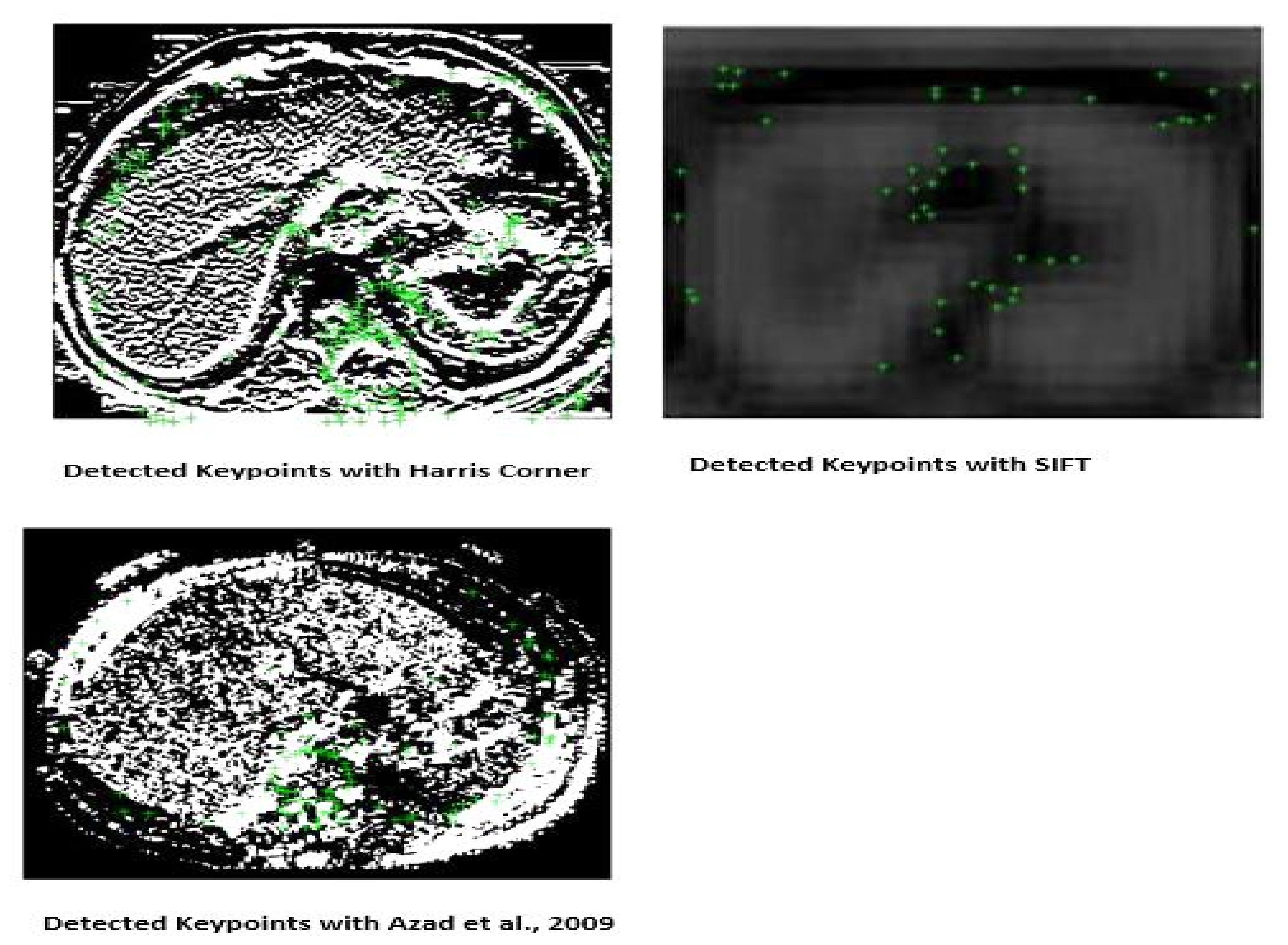
3.2.1. Detection of Harris Corner

The mathematical interpretation of the Harris corner is as follows:

$$E(u,v)=\sum _{x,y}w(x,y){\left[I(x+u,y+v)-I(x,y)\right]}^2,$$

(1)

where,

• The difference between the original and transferred window is represented by E,
• the x-axis shift of the window is represented by u,
• The y-axis shift of the windows is represented by v,
• The window at (x, y) is represented by w(x, y). This appears to be a mask. Which ensures that only the appropriate window is used,
• The window function is represented by ${\sum }_{\mathit{x},\mathit{y}}$ w(x,y),
• The shifted intensity is represented by I(x+u,y+v) and the intensity at (x,y) is represented by I(x,y).

We have to maximize the equation above, because we are looking for windows with corners, i.e., windows with a lot of intensity variation will be considered. Particularly the term: ${\left[I(x+u,y+v)-I(x,y)\right]}^2$ by using the Taylor expansion as:

$$\begin{array}{c}\hfill E(u,v)\approx \sum _{x,y}w(x,y)(u^2{I}_x^2+2uv{I}_x{I}_y+v^2{I}_y^2)\\ \hfill =(u,v)\left(\sum _{x,y}w(x,y)\left[\begin{array}{cc}{I}_x^2& I_x{I}_y\\ I_x{I}_y& I_y^2\end{array}\right]\right)\left(\begin{array}{c}u\\ v\end{array}\right)\\ \hfill =(u,v)M\left(\begin{array}{c}u\\ v\end{array}\right)\end{array}$$

(2)

The bilinear approximation for the average intensity change in direction $\left[u,v\right]$ as follows:

$$E(u,v)\approx \left[uv\right]M\left[\begin{array}{c}u\\ v\end{array}\right],$$

(3)

where M is a structure tensor of a pixel, which is a $2\times 2$ matrix. It is a characterization of information of all pixels within the window where, (I${}_{{}_x}^2,{\mathit{I}}_{{}_x}{\mathit{I}}_y),({\mathit{I}}_{{}_x}{\mathit{I}}_y,{\mathit{I}}_{{}_y}^2)$ are the partial derivatives in x and y.

Furthermore, after that, as a measure of corner response a point is described in terms of eigenvalues, ${\lambda }_1{\lambda }_2$, of M, as follows:

$$H=det\left(M\right)-k{\left(tr\left(M\right)\right)}^2,$$

(4)

with $det\left(M\right)={\lambda }_1{\lambda }_2$, $tr\left(M\right)={\lambda }_1+{\lambda }_2$. Here $det(.)$ and $tr(.)$ are the determinant and trace, respectively.

In order to figure out why matrix M has the capacity to determine the corner’s characteristic, we computed the covariance matrix $\mathsf{\Sigma }$ of gradient $(I_x,I_y)$ at a pixel. Let ${\mu }_x=E\left[I_x\right],{\mu }_y=E\left[I_y\right]$. So by the definition of covariance matrix we have:

$$\begin{array}{c}\hfill \begin{array}{cc}\hfill \mathsf{\Sigma }& =\left[\begin{array}{cc}E\left[(I_x-{\mu }_x)(I_x-{\mu }_x)\right]& E\left[(I_x-{\mu }_x)(I_y-{\mu }_y)\right]\\ E\left[(I_y-{\mu }_y)(I_x-{\mu }_x)\right]& E\left[(I_y-{\mu }_y)(I_y-{\mu }_y)\right]\end{array}\right]\hfill \\ & =\left[\begin{array}{cc}E\left[I_x{I}_x\right]-{\mu }_x^2& E\left[I_x{I}_y\right]-{\mu }_x{\mu }_y\\ E\left[I_y{I}_x\right]-{\mu }_y{\mu }_x& E\left[I_y{I}_y\right]-{\mu }_y^2\end{array}\right]\hfill \\ & \triangleq \left[\begin{array}{cc}E\left[I_x{I}_x\right]& E\left[I_x{I}_y\right]\\ E\left[I_y{I}_x\right]& E\left[I_y{I}_y\right]\end{array}\right]\hfill \end{array}\end{array}$$

(5)

On the other hand, matrix M is as follows if we apply an averaging filter over the time dimension by giving the uniform weight over the pixels within the pixels:

$$\begin{array}{cc}\hfill M& =\frac{1}{f}\sum _{x,y}\left[\begin{array}{cc}{I}_x^2& I_x{I}_y\\ I_x{I}_y& I_y^2\end{array}\right]\hfill \\ & =\left[\begin{array}{cc}\widehat{I_x^2}& \widehat{I_x{I}_y}\\ \widehat{I_x{I}_y}& \widehat{I_y^2}\end{array}\right]\hfill \end{array},$$

(6)

where f is the total number of pixels within the window.

From the above equations, it can be seen that the matrix M is actually an unbiased estimate of the covariance matrix of the gradients for the pixels within the window. Therefore findings in the covariance matrix of the gradients calculated in Equation (5) can be used to analyze the structure tensors.

A good corner has a large intensity change in all directions [13], i.e., H should be a large positive number. We obtain the image derivatives by convolving it with the derivative masks and then smoothing these image derivatives with the Gaussian filter to compute the Harris corner response while keeping the basic working principle of Harris corner in consideration.

The pixels that are not part of the local maxima are then set to zero using non-maximal suppression. This allows us to extract the local maxima by dilation, then find the points in the corner strength image that match the dilated image, and finally obtain the coordinates, which are referred to as keypoints. Figure 5 summarizes the output of each step in Harris corner detection.

Each stage in Figure 5 is obtained in the mathematical formulation as following steps:

• computing image derivatives: $I_x$ and $I_y$ are obtained by computing the x and y derivatives as:

  $$I_x=G_{\sigma }^x\times I$$

  (7)

  $$I_y=G_{\sigma }^y\times I$$

  (8)
• Calculate derivative products at each pixel as:

  $$I_x^2=I_x\times I_x$$

  (9)

  $$I_y^2=I_y\times I_y$$

  (10)

  $$I_{xy}=I_x\times I_y$$

  (11)
• Finally, the response of the detector at each pixel is computed as:

  $$H=det\left(M\right)-k{\left(tr\left(M\right)\right)}^2,$$

  (12)

In order to see the discriminating capability of adopting Harris corner as a starting point for keypoint detection, the comparison in the first two steps of SIFT and Harris corner were analyzed. The output of scale space extrema of the SIFT descriptor is shown in Figure 6.

As can be seen in Figure 6, the scale space extrema process in the fourth octave loses the details about an image as it is unable to determine the actual fine details of the image which results in fewer keypoints as shown in Figure 7. These characteristics are important in classifying images with variability as compared to Figure 5, in which fine details of the images are still preserved even if it is subjected to low resolution. Furthermore, it can be seen in Figure 7, that the keypoints detected by Harris corner capture the maximum shape of the object which will help in better classification. Medical images with low resolution will not be classified with only the SIFT process because of the loss of details as it progresses through the different octaves.

3.2.2. Key Points Orientation Assignment

Following the extraction of the Harris corners, the next step in the SIFT algorithm is orientation assignment, which involves determining ascendant orientations for each keypoint based on its local gradient direction. This is accomplished by creating a 36-bin histogram from the image gradients around the keypoint. Each keypoint is normalized by aligning it to the direction of its orientation, as determined by the following equations.

$$\begin{array}{c}\hfill H_x=H(x+1,y)-H(x-1,y),\\ \hfill H_y=H(x,y+1)-H(x,y-1),\\ \hfill m(x,y)=\sqrt{{\left(H_x\right)}^2+{\left(H_y\right)}^2}.\end{array}$$

(13)

$$\theta (x,y)=ta{n}^{-1}\left(\frac{H(x,y+1)-H(x,y-1)}{H(x+1,y)-H(x-1,y)}\right),$$

(14)

where, $m(x,y)$ and $\theta (x,y)$ are the gradient magnitude and orientation of pixel (x,y) and H is the Hessian measure. The orientation of the computed features is shown in Figure 8.

The last step is to create a keypoint descriptor, which computes the local image descriptor based on the image gradients in its immediate vicinity. The area surrounding the keypoint is divided into $4\times 4$ sub-regions. For each sub-region, an orientation histogram with eight bins is constructed, yielding a $4\times 4\times 8=128$ dimensional vector for each region. The process is summarized as shown in Figure 9.

3.3. Construction of the Codebook

Encoding and pooling are the two steps in the construction of a bag of visual words (BOVW) representation. The local descriptors are encoded into codebook elements in the encoding step, and the codebook elements are aggregated into a vector in the pooling step.

The encoding step is the vital component, because it links the feature extraction and feature pooling and has a great impact on the image classification in terms of accuracy and speed. The most commonly used encoding step is vector quantization(VQ) [47]. The problem with this encoding method is that it assigns each descriptor to a single visual word, which results in quantization loss and it also ignores the relationship between different bases. In the case of medical images, this limitation imposes a constraint on feature encoding because medical image datasets are high dimensional and often represent complex nonlinear phenomena. To overcome this, an encoding method of Locality constraint Linear Coding(LLC) [48] is used, which achieves fewer reconstruction errors by using multiple bases.

In LLC, the least squares fitting problem is solved by the the following equation:

$$argmi{n}_k\sum _{i=1}^N\left|\right|z_i-M_{k_i}{\left|\right|}^{{}^2}+\lambda \left|\right|d_i\odot k_i{\left|\right|}^2,$$

(15)

where k $=[k_1,k_2,.....,k_N]$ is the set of codes for local descriptors z $=[z_1,z_2,.....zN]$. Furthermore, $d_i$ is the locality constraint, which is given as:

$$d_i=\left(\frac{dist(z_i,M)}{\sigma }\right),$$

(16)

where $dist(z_i,M)=dist[dist(z_i,b_1),......dist{(x_i,b_M]}^T$. $\sigma$ is the weight decay speed adjuster for locality constraint.

3.4. Ensemble Classifier with Surrogate Splits

An ensemble classifier consists of a set of individually trained classifiers whose predictions are combined for classifying new instances [49]. Ensemble classifier with surrogate splits [15] may help in minimizing the generalization error by handling the missing values which occurred due to the noisy data in some anatomical classes. Moreover, it has been stated that tree based ensembles handle high dimensional data easily [50]. Surrogate splits can be used to estimate the value of a missing feature based on the value of a feature with which it is highly correlated.

Bagging

By training each classifier on the random distribution of the training set [51], as a bootstrap pooling method generates replacements for its ensemble. Each classifier’s training set is created by resampling the training set with replacement. A sequence of decision tree classifiers $C_m$, $m=1,2,\cdots ,M$ is created. After that, an ensemble classifier is created by combining the individual classifiers. The basic formulation of bagging is given in Algorithm 1.

Algorithm 1: Bagging Algorithm

Input:training set S, Decision Tree I, integer T (number of bootstrap samples).

1: for i : = 1 to T do

2:          S’ = bootstrap sample from S

3:          Ci = I’(S’)

4 : end for

5: $C_m^{*}={\mathrm{argmax}}_{y\in Y}\sum _{i:C_i\left(m\right)=y}1$ (the most often predicted label y)

Output: classifier C*

When two features have a high correlation, surrogates estimate the value of missing attributes based on the feature with which they are highly correlated. If an attribute’s value is missing, the mean of all instances with the same estimated class value, i.e., the mean of the instances from the same class label, is used to estimate it.

In addition to this, surrogate splits have also shown good performance in handling both training and testing missing cases as reported in [50].

Our modified algorithm using bagging with surrogate splits is given in Algorithm 2.

Algorithm 2: Bagging with surrogate splits

1: procedure BAGALGO ()

2:    Initialize training set T

3:    for n = 1,.....,N do

4:       Create a surrogate split X,X ≤ sX, bootstrap replica by randomly sampling with replacement on training set T.

5:       Learn m individual classifiers Cm

6:       Create an ensemble classifier by aggregating individual classifiers Cm: m = 1,.....,M

7:       Classify sample ti to class sj according to the number of votes obtained from classifiers.

8:    end for

9: end procedure

4. Comparative Results for HSIFT and CNN and Experiment

We began our experiments with a machine equipped with an NVIDIA GeForce GTX 980M graphics card and a data set obtained from the National Institutes of Health, Department of Health and Human Services [11] as mentioned in Section 3.1.

4.1. Experimental Setup for HSIFT

Our experiments were run with 10-fold cross-validation. Various codebook sizes were empirically experimented, and the optimal codebook size for anatomy recognition found is 500 as shown in Figure 10. Hence, the dimension of the BOVW(HSIFT) adopted is 500 for each image instance.

We conducted a thorough experiment on SIFT [52], SIFT + Harris corner [39] and BOVW(HSIFT) by applying the SVM and also the ensemble classifiers. As shown in

Table 1. Results of 10-fold cross validation on training dataset with SIFT, HSIFT, BOVW(HSIFT).

Feature Representation	SVM Error Rate %	Regular Bagging Error Rate %	Bagging with Surrogate Splits Error Rate %
SIFT [52]	29.0	26.6	23.0
SIFT + Harris corner [39]	30.0	28.6	26.4
BOVW(SIFT) [53]	20.5	33.2	33.4
BOVW(HSIFT)	9.7	3.0	2.0

, it was found that BOVW(HSIFT) outperformed the SIFT+Harris corner [39] and BOVW(SIFT) [53] although the latter had shown good matching in natural images and modality classification, respectively, from their work. It is also shown that BOVW(HSIFT) performed the best among all the tested features, which produced only 9.7% error rate by using SVM and 2% using bagging with surrogate splits classification technique. The results are summarized in Table 1.

Experiments on regular bagging and bagging with surrogate splits with $M=[1,50]$ were conducted to see how different numbers of trees affected cross-validation errors in order to determine the optimal number of trees, M, to be used in the testing stage. It can be seen from the experiment results in Figure 11 that the minimum cross-validation error was achieved at $M=50$. Taking this into account, during the testing stage, bagging with surrogate splits of 50 trees was chosen as the best option. For bagging with surrogate splits, the cross-validated error is 2%.

After analyzing the cross-validation results we test the trained model on the test data set of 500 images. The results of which are shown in Figure 12. It clearly shows that the proposed method outperforms the regular bagging, which results in 98.1% accuracy.

The ROC curve for the diagnostic test evaluation of the proposed feature is as shown in Figure 13. It depicts the AUC of 0.98 indicating good performance of the method.

4.2. Experimental Setup for Convolutional Neural Network (CNN)

CNN has found a cutting edge capability in different competitions in computer vision and image recognition [54]. In order to leverage the effectiveness of CNN for medical image anatomy classification, we need to analyze the comparative performance of our proposed features and CNN features to investigate the discrimination power between those two methods.

An evaluation metric, normalized mutual information, that helps in determining the discriminative capacity of these two feature extraction methods was adopted in order to quantitatively analyze the discriminative capacity of the feature maps. The experiments were conducted based on calculations of entropy and mutual information.

Let L be the category label and F represents the features. The entropy $H(.)$ is calculated as the amount of uncertainty for a partition set assuming two label assignments $(L,F)$ are defined as:

$$H\left(L\right)=\sum _{i=1}^{\left|L\right|}P\left(i\right)log\left(P\left(i\right)\right),$$

(17)

where $P\left(i\right)=\left|L\right|N$ is the probability that an instance picked at random from L fall in class $L_i$.

Similarly for F:

$$\mathrm{H}\left(F\right)=\sum _{j=1}^{\left|F\right|}{P}^{\prime }\left(j\right)log\left(P^{\prime }\left(j\right)\right),$$

(18)

where $P^{\prime }\left(j\right)=\left|F\right|N$ is the probability that an instance picked at random from F fall in class $F_j$.

The mutual information between $(L,F)$ is calculated as:

$$\mathrm{MI}(L,F)=\sum _{i=1}^{\left|L\right|}\sum _{j=1}^{\left|F\right|}P(i,j)log\left(\frac{P(i,j)}{\left(P\left(i\right)P^{\prime }\left(j\right)\right)}\right).$$

(19)

Based on Equations (17)–(19), normalized mutual information [55] is defined as:

$$\mathrm{NMI}(L,F)=\frac{MI(L,F)}{\sqrt{H\left(L\right)H\left(F\right)}},$$

(20)

where $MI(L,F)$ is the mutual information between category label L and feature map activations F. $H(.)$ is the entropy and $\sqrt{H\left(L\right)H\left(F\right)}$ is used for normalizing the mutual information to be in the range of $[0,1]$.

Table 2. Normalized Mutual Information for LeNet, AlexNet and GoogLeNet.

Layers	LeNet	AlexNet	GoogLeNet
conv-1	0.22	0.66	0.56
conv-2	0.28	0.70	0.62
conv-3	-	0.74	0.51
conv-4	-	0.75	0.53
ip2/fc8/pool5/$7\times 7\_s1$	0.30	0.79	0.63
HSIFT	0.93	0.93	0.93

shows the computed Normalized Mutual Information (NMI) for architectures used in this study. The layers, i.e., ip2/fc8/pool5/$7\times 7\_s1$ represent the last fully connected layers of the three milestone architectures, respectively. A normalized mutual information score close to value 1 depicts strong correlation between the output activations and category labels while an NMI score close to zero depicts bad correlation. It is evident from the results in Table 2 that the proposed HSIFT feature outperforms the CNN’s feature in terms of discriminative power of features in depicting the category labels.

Table 3. In terms of runtime, training loss, validation accuracy and test accuracy, comparative performance of LeNet, AlexNet and GoogLenet with proposed CNN.

Model	Runtime in Seconds	Validation Loss	Validation Accuracy	Test Accuracy
LeNet [56]	1655	1.3	58.0	59.0
AlexNet [54]	33,466	1.39	65.0	74.0
GoogLeNet [57]	52,470	1.2	55.0	45.0
SIFT + Harris corner [39]	648	26.4	73.6	73.8
HSIFT-LBP [36]	328	0.21	79.0	64.0
Optimized CNN	16,728	0.67	76.6	81.0
Proposed BOVW(HSIFT)	235	0.02	98.0	98.1

summarizes the performance of the proposed HSIFT feature versus the three milestone architectures in terms of runtime, training loss, validation accuracy, and test accuracy. Because these three landmark architectures were used for natural image classification, the parameter tuning and layer formulation required a more subtle approach. Even with optimized CNN architecture tuning, the HSIFT feature still outperforms deep learned features in terms of discriminating ability.

The normalization function and subtle tuning of hyper parameters will yield better results for the task of medical image anatomy classification with the modification of basic CNN architecture in terms of number of layers. Nevertheless, results from Table 2 revealed, that the architectures used for natural image classification cannot be applied to medical image objects or anatomies. The few misclassified instances out of 500 images are shown in Figure 14.

As it can be seen from the Figure 14, that the shape of the organ and its intensity plays an important role in discriminating the anatomical structures.

5. Conclusions

We proposed a modified SIFT descriptor with Harris corner to form the Bag-Of-Visual-Words feature in image representations in this paper. The use of Harris corner to replace the first two steps of SIFT process has the advantage of assigning orientation to each keypoint that provides rotation invariance while at the same time helps to deal with viewpoint changes. As anatomical images are sometimes captured from different viewpoints, this is important in distinguishing between them. The combination of these primitive descriptors results in a more discriminative codebook in the BOVW representation, allowing for efficient anatomy classification while remaining robust to transformations. When compared to the traditional SVM classification technique, which is commonly used in classifying medical images, the use of an ensemble classifier that is Bagging with surrogate splits is good at handling missing data and improving classification accuracy.

The proposed ensemble descriptor outperforms some previous work in medical image anatomy, according to the experiments. Even with different modalities, it aids in the creation of more discriminative codebooks for anatomy classification. In comparison to convolutional neural networks, the proposed ensemble classifier of bagging with surrogate splits provides better discrimination power in extraction features. It also concludes that at the current stage, a Convolutional Neural Network does not guarantee its success in general medical image classification with various settings from moderate data sizes of a few tens of thousands, only. The work can be expanded in the future to include the recognition and classification of pathological structures from these anatomies, resulting in a fully automated medical image classification system.

References

1. Zhou, X.; Depeursinge, A.; Müller, H. Hierarchical classification using a frequency-based weighting and simple visual features. Pattern Recognit. Lett. 2008, 29, 2011–2017. [Google Scholar] [CrossRef]
2. Tommasi, T.; Orabona, F.; Caputo, B. Discriminative cue integration for medical image annotation. Pattern Recognit. Lett. 2008, 29, 1996–2002. [Google Scholar] [CrossRef] [Green Version]
3. Kalpathy-Cramer, J.; Hersh, W. Effectiveness of global features for automatic medical image classification and retrieval–The experiences of OHSU at ImageCLEFmed. Pattern Recognit. Lett. 2008, 29, 2032–2038. [Google Scholar] [CrossRef] [PubMed] [Green Version]
4. Avni, U.; Greenspan, H.; Konen, E.; Sharon, M.; Goldberger, J. X-ray categorization and retrieval on the organ and pathology level, using patch-based visual words. Med. Imaging IEEE Trans. 2011, 30, 733–746. [Google Scholar] [CrossRef] [PubMed]
5. Depeursinge, A.; Vargas, A.; Platon, A.; Geissbuhler, A.; Poletti, P.; Müller, H. 3D case–based retrieval for interstitial lung diseases. Med-Content-Based Retr. Clin. Decis. Support 2010, 5853, 39–48. [Google Scholar]
6. Rahman, M.; Davis, D. Addressing the class imbalance problem in medical datasets. Int. J. Mach. Learn. Comput. 2013, 3, 224–228. [Google Scholar] [CrossRef]
7. Song, Y.; Cai, W.; Huang, H.; Zhou, Y.; Wang, Y.; Feng, D. Locality-constrained Subcluster Representation Ensemble for lung image classification. Med. Image Anal. 2015, 22, 102–111. [Google Scholar] [CrossRef] [Green Version]
8. Srinivas, M.; Naidu, R.; Sastry, C.; Mohan, C. Content based medical image retrieval using dictionary learning. Neurocomputing 2015, 168, 880–895. [Google Scholar] [CrossRef]
9. Magdy, E.; Zayed, N.; Fakhr, M. Automatic classification of normal and cancer lung CT images using multiscale AM-FM features. J. Biomed. Imaging 2015, 2015, 11. [Google Scholar] [CrossRef] [Green Version]
10. Chen, D.; Chang, R.; Chen, C.; Ho, M.; Kuo, S.; Chen, S.; Hung, S.; Moon, W. Classification of breast ultrasound images using fractal feature. Clin. Imaging 2005, 29, 235–245. [Google Scholar] [CrossRef]
11. Roth, H.; Lee, C.; Shin, H.; Seff, A.; Kim, L.; Yao, J.; Lu, L.; Summers, R. Anatomy-specific classification of medical images using deep convolutional nets. In Proceedings of the 2015 IEEE 12th International Symposium On Biomedical Imaging (ISBI), New York, NY, USA, 16–19 April 2015; pp. 101–104. [Google Scholar]
12. Lyndon, D.; Kumar, A.; Kim, J.; Leong, P.; Feng, D. Convolutional Neural Networks for Medical Clustering. Ceur Workshop Proc. 2015. Available online: http://ceur-ws.org/Vol-1391/52-CR.pdf (accessed on 21 September 2021).
13. Harris, C.; Stephens, M. A combined corner and edge detector. Alvey Vis. Conf. 1988, 15, 50. [Google Scholar]
14. Lowe, D. Object recognition from local scale-invariant features. In Proceedings of the Seventh IEEE International Conference On Computer Vision, Kerkyra, Greece, 20–27 September 1999; pp. 1150–1157. [Google Scholar]
15. Feelders, A. Handling missing data in trees: Surrogate splits or statistical imputation? In Proceedings of the European Conference on Principles of Data Mining and Knowledge Discovery, Prague, Czech Republic, 15–18 September 1999; pp. 329–334. [Google Scholar]
16. Tartar, A.; Akan, A. Ensemble learning approaches to classification of pulmonary nodules. In Proceedings of the 2016 International Conference On Control, Decision Furthermore, Information Technologies (CoDIT), Saint Julian, Malta, 6–8 April 2016; pp. 472–477. [Google Scholar]
17. Xia, J.; Zhang, S.; Cai, G.; Li, L.; Pan, Q.; Yan, J.; Ning, G. Adjusted weight voting algorithm for random forests in handling missing values. Pattern Recognit. 2017, 69, 52–60. [Google Scholar] [CrossRef]
18. Zare, M.; Mueen, A.; Seng, W. Automatic medical X-ray image classification using annotation. J. Digit. Imaging 2014, 27, 77–89. [Google Scholar] [CrossRef] [Green Version]
19. Kumar, A.; Dyer, S.; Li, C.; Leong, P.; Kim, J. Automatic Annotation of Liver CT Images: The Submission of the BMET Group to ImageCLEFmed 2014. In Proceedings of the CLEF (Work. Notes), Sheffield, UK, 15–18 September 2014; pp. 428–437. [Google Scholar]
20. Yang, W.; Lu, Z.; Yu, M.; Huang, M.; Feng, Q.; Chen, W. Content-based retrieval of focal liver lesions using bag-of-visual-words representations of single-and multiphase contrast-enhanced CT images. J. Digit. Imaging 2012, 25, 708–719. [Google Scholar] [CrossRef] [PubMed] [Green Version]
21. Désir, C.; Petitjean, C.; Heutte, L.; Thiberville, L.; Salaün, M. An SVM-based distal lung image classification using texture descriptors. Comput. Med. Imaging Graph. 2012, 36, 264–270. [Google Scholar] [CrossRef] [PubMed] [Green Version]
22. Lecron, F.; Benjelloun, M.; Mahmoudi, S. Descriptive image feature for object detection in medical images. In Proceedings of the International Conference Image Analysis and Recognition, Aveiro, Portugal, 25–27 June 2012; pp. 331–338. [Google Scholar]
23. Sargent, D.; Chen, C.; Tsai, C.; Wang, Y.; Koppel, D. Feature detector and descriptor for medical images. SPIE Med. Imaging 2009, 7259, 72592Z. [Google Scholar]
24. Cui, J.; Xie, J.; Liu, T.; Guo, X.; Chen, Z. Corners detection on finger vein images using the improved Harris algorithm. Opt.-Int. J. Light Electron Opt. 2014, 125, 4668–4671. [Google Scholar] [CrossRef]
25. Kim, H.; Shin, S.; Wang, W.; Jeon, S. SVM-based Harris corner detection for breast mammogram image normal/abnormal classification. In Proceedings of the 2013 Research in Adaptive and Convergent Systems, Montreal, QC, Canada, 1–4 October 2013; pp. 187–191. [Google Scholar]
26. Shim, J.; Park, K.; Ko, B.; Nam, J. X-Ray image classification and retrieval using ensemble combination of visual descriptors. In Proceedings of the Pacific-Rim Symposium on Image and Video Technology, Tokyo, Japan, 13–16 January 2009; pp. 738–747. [Google Scholar]
27. Taheri, M.; Hamer, G.; Son, S.; Shin, S. Enhanced Breast Cancer Classification with Automatic Thresholding Using SVM and Harris Corner Detection. In Proceedings of the International Conference on Research in Adaptive and Convergent Systems, Odense, Denmark, 11–14 October 2016; pp. 56–60. [Google Scholar]
28. Lee, C.; Wang, H.; Chen, C.; Chuang, C.; Chang, Y.; Chou, N. A modified Harris corner detection for breast IR image. Math. Probl. Eng. 2014, 2014, 902659. [Google Scholar] [CrossRef] [Green Version]
29. Gao, L.; Pan, H.; Han, J.; Xie, X.; Zhang, Z.; Zhai, X. Corner detection and matching methods for brain medical image classification. In Proceedings of the 2016 IEEE International Conference On Bioinformatics Biomedicine (BIBM), Shenzhen, China, 15–18 December 2016; pp. 475–478. [Google Scholar]
30. Zhou, D.; Gao, Y.; Lu, L.; Wang, H.; Li, Y.; Wang, P. Hybrid corner detection algorithm for brain magnetic resonance image registration. In Proceedings of the 2011 4th International Conference On Biomedical Engineering Furthermore, Informatics (BMEI), Shanghai, China, 15–17 October 2011; pp. 308–313. [Google Scholar]
31. Biswas, B.; Dey, K.; Chakrabarti, A. Medical image registration based on grid matching using Hausdorff Distance and Near set. In Proceedings of the 2015 Eighth International Conference On Advances In Pattern Recognition (ICAPR), Kolkata, India, 4–7 January 2015; pp. 1–5. [Google Scholar]
32. Zhang, R.; Zhou, W.; Li, Y.; Yu, S.; Xie, Y. Nonrigid registration of lung CT images based on tissue features. Comput. Math. Methods Med. 2013, 2013, 834192. [Google Scholar] [CrossRef]
33. Chen, J.; Tian, J.; Lee, N.; Zheng, J.; Smith, R.; Laine, A. A partial intensity invariant feature descriptor for multimodal retinal image registration. IEEE Trans. Biomed. Eng. 2010, 57, 1707–1718. [Google Scholar] [CrossRef] [Green Version]
34. Gharabaghi, S.; Daneshvar, S.; Sedaaghi, M. Retinal image registration using geometrical features. J. Digit. Imaging 2013, 26, 248–258. [Google Scholar] [CrossRef] [Green Version]
35. Jin, D.; Zhu, S.; Cheng, Y. Salient object detection via harris corner. In Proceedings of the 2017 29th Chinese Control And Decision Conference (CCDC), Chongqing, China, 28–30 May 2017; pp. 1108–1112. [Google Scholar]
36. Khan, S.; Yong, S.; Deng, J. Ensemble classification with modified SIFT descriptor for medical image modality. In Proceedings of the 2015 International Conference On Image Furthermore, Vision Computing New Zealand (IVCNZ), Auckland, New Zealand, 23–24 November 2015; pp. 1–6. [Google Scholar]
37. Benjelloun, M.; Mahmoudi, S.; Lecron, F. A framework of vertebra segmentation using the active shape model-based approach. J. Biomed. Imaging 2011, 2011, 9. [Google Scholar] [CrossRef]
38. Yan, Z.; Zhang, J.; Zhang, S.; Metaxas, D. Automatic Rapid Segmentation of Human Lung from 2D Chest X-Ray Images. In Proceedings of the Miccai Workshop Sparsity Tech. Med Imaging, Nice, France, 12–16 October 2012; pp. 1–8. [Google Scholar]
39. Azad, P.; Asfour, T.; Dillmann, R. Combining Harris interest points and the SIFT descriptor for fast scale-invariant object recognition. In Proceedings of the IROS 2009. IEEE/RSJ International Conference On Intelligent Robots Furthermore Systems, St. Louis, MO, USA, 10–15 October 2009; pp. 4275–4280. [Google Scholar]
40. Yang, M.; Yuan, Y.; Li, X.; Yan, P. Medical Image Segmentation Using Descriptive Image Features. BMVC. 2011, pp. 1–11. Available online: https://citeseerx.ist.psu.edu/viewdoc/download?doi=10.1.1.297.9559&rep=rep1&type=pdf (accessed on 21 September 2021).
41. Moradi, M.; Abolmaesoumi, P.; Mousavi, P. Deformable registration using scale space keypoints. Med. Imaging 2006, 6144, 61442G. [Google Scholar]
42. Cireşan, D.; Giusti, A.; Gambardella, L.; Schmidhuber, J. Mitosis detection in breast cancer histology images with deep neural networks. In Proceedings of the International Conference on Medical Image Computing and Computer-Assisted Intervention, Nagoya, Japan, 22–26 September 2013; pp. 411–418. [Google Scholar]
43. Prasoon, A.; Petersen, K.; Igel, C.; Lauze, F.; Dam, E.; Nielsen, M. Deep feature learning for knee cartilage segmentation using a triplanar convolutional neural network. In Proceedings of the International Conference on Medical Image Computing and Computer-Assisted Intervention, Nagoya, Japan, 22–26 September 2013; pp. 246–253. [Google Scholar]
44. Roth, H.; Lu, L.; Seff, A.; Cherry, K.; Hoffman, J.; Wang, S.; Liu, J.; Turkbey, E.; Summers, R. A new 2.5 D representation for lymph node detection using random sets of deep convolutional neural network observations. In Proceedings of the International Conference on Medical Image Computing and Computer-Assisted Intervention, Boston, MA, USA, 14–18 September 2014; pp. 520–527. [Google Scholar]
45. Li, Q.; Cai, W.; Wang, X.; Zhou, Y.; Feng, D.; Chen, M. Medical image classification with convolutional neural network. In Proceedings of the 2014 13th International Conference On Control Automation Robotics & Vision (ICARCV), Marina Bay Sands, Singapore, 10–12 December 2014; pp. 844–848. [Google Scholar]
46. Cho, J.; Lee, K.; Shin, E.; Choy, G.; Do, S. Medical Image Deep Learning with Hospital PACS Dataset. arXiv 2015, arXiv:1511.06348. [Google Scholar]
47. Csurka, G.; Dance, C.; Fan, L.; Willamowski, J.; Bray, C. Visual categorization with bags of keypoints. Workshop Stat. Learn. Comput. Vis. 2004, 1, 1–2. [Google Scholar]
48. Wang, J.; Yang, J.; Yu, K.; Lv, F.; Huang, T.; Gong, Y. Locality-constrained linear coding for image classification. In Proceedings of the 2010 IEEE Conference On Computer Vision Furthermore, Pattern Recognition (CVPR), San Francisco, CA, USA, 13–18 June 2010; pp. 3360–3367. [Google Scholar]
49. Claesen, M.; De Smet, F.; Suykens, J.; De Moor, B. EnsembleSVM: A library for ensemble learning using support vector machines. J. Mach. Learn. Res. 2014, 15, 141–145. [Google Scholar]
50. Valdiviezo, H.; Van Aelst, S. Tree-based prediction on incomplete data using imputation or surrogate decisions. Inf. Sci. 2015, 311, 163–181. [Google Scholar] [CrossRef]
51. Breiman, L. Bagging predictors. Mach. Learn. 1996, 24, 123–140. [Google Scholar] [CrossRef] [Green Version]
52. Zare, M.; Mueen, A.; Seng, W. Automatic classification of medical X-ray images using a bag of visual words. Comput. Vis. IET 2013, 7, 105–114. [Google Scholar] [CrossRef]
53. Gál, V.; Kerre, E.; Nachtegael, M. Multiple kernel learning based modality classification for medical images. In Proceedings of the 2012 IEEE Computer Society Conference On Computer Vision Furthermore, Pattern Recognition Workshops (CVPRW), Providence, RI, USA, 16–21 June 2012; pp. 76–83. [Google Scholar]
54. Krizhevsky, A.; Sutskever, I.; Hinton, G. Imagenet classification with deep convolutional neural networks. Adv. Neural Inf. Process. Syst. 2012, 25, 1097–1105. [Google Scholar] [CrossRef]
55. Chen, W.; Song, Y.; Bai, H.; Lin, C.; Chang, E. Parallel spectral clustering in distributed systems. IEEE Trans. Pattern Anal. Mach. Intell. 2011, 33, 568–586. [Google Scholar] [CrossRef] [PubMed]
56. LeCun, Y.; Bottou, L.; Bengio, Y.; Haffner, P. Gradient-based learning applied to document recognition. Proc. IEEE 1998, 86, 2278–2324. [Google Scholar] [CrossRef] [Green Version]
57. Szegedy, C.; Liu, W.; Jia, Y.; Sermanet, P.; Reed, S.; Anguelov, D.; Erhan, D.; Vanhoucke, V.; Rabinovich, A. Going deeper with convolutions. In Proceedings of the IEEE Conference on Computer Vision and Pattern Recognition, Boston, MA, USA, 7–12 June 2015; pp. 1–9. [Google Scholar]
Figure 1. Example images of visual variability even though from the similar anatomy object classes, i.e., heart and kidney (a) CT heart, (b) MRI heart, (c) CT kidney, (d) MRI kidney.
Symmetry 13 01987 g001
Figure 2. Schematic for medical image classification.
Symmetry 13 01987 g002
Figure 3. Various transformations applied to medical images, for instance, illumination, rotation, blurring and compression. (a) Illumination; (b) Rotation; (c) Blurring; (d) Compression.
Symmetry 13 01987 g003
Figure 4. Images of five anatomies from various modalities as examples. The first row corresponds to the CT modality, the second row to the MRI modality, and the third row to the PET modality.
Symmetry 13 01987 g004
Figure 5. Process of Harris detector.
Symmetry 13 01987 g005
Figure 6. Process of scale space extrema in SIFT.
Symmetry 13 01987 g006
Figure 7. Detected keypoints with Harris and SIFT, respectively.
Symmetry 13 01987 g007
Figure 8. Orientation of detected corners.
Symmetry 13 01987 g008
Figure 9. Process of HSIFT descriptor.
Symmetry 13 01987 g009
Figure 10. Classification accuracy with the increasing codebook size for Locality-Constrained Linear Voding and Vector Quantization with increasing codebook size.
Symmetry 13 01987 g010
Figure 11. Comparative analysis of cross-validated error for training data.
Symmetry 13 01987 g011
Figure 12. Error analysis for test data using regular bagging versus bagging with surrogate splits.
Symmetry 13 01987 g012
Figure 13. ROC curve for the proposed method.
Symmetry 13 01987 g013
Figure 14. Misclassified instances of heart as lung, kidney and lumbarspine. (a) heart misclassified as lung; (b) heart misclassified as kidney; (c) heart misclassified as lumberspine; (d) heart misclassified as lung.
Symmetry 13 01987 g014