1. Introduction
The dynamical system of the restricted three-body problem (RTBP) has a significant role in celestial mechanics. It has many applications in the astrodynamics and stellar dynamics fields [
1,
2,
3,
4]. The RTBP is a special case of three-body problem whereas the restricted four-body (RFBP) problem is a generalization of the RTBP. In the RTBP, both primaries circumambulate around their common center of mass while the infinitesimal body does not have gravitational influence on the primaries bodies.
Several studies have been carried out on the RTBP to analyze infinitesimal body motion [
5,
6,
7,
8]. Further considerable work in the frame of perturbed RTBP was undertaken in [
9,
10] to explore the equilibrium points, linear stability and feature of motion about these points.
One of the major features of the RTBP is that it can be reduced to some simpler models, which also has massive significance in celestial mechanics—including but not limited to Hill’s system [
11,
12,
13], Robe’s model [
14,
15] and the Sitnikov problem [
6,
16]. However, the Sitnikov problem is considered the simplest model as it is a reduced model of the three-body problem which can be obtained as a sub-case of the circular or elliptic RTBP where the infinitesimal body oscillates along the perpendicular to the plane of the primaries—which is the
Z axis. Moreover, it is considered as the simplest sub-case of the
body problem, and in many cases it can be used as a first approximation for astronomical problems in real situations.
In the Sitnikov problem, the existence of oscillation motion was first proven by [
17]. Recently, the effect of the gravitational radius in the sense of chaotic scattering phenomenon and the escape regions were studied under the relativistic effect. Furthermore, inflection points in a quantitative behavior were analyzed by using the basin entropy [
18]. The Sitnikov problem is also generalized in the sense that the primary bodies’ motions are homographic and form over a long time following a permissible central configuration [
19]. The author has studied the continuation of the global periodic solutions for all eccentricity values in the interval
.
The major motivation of the current study was that the Sitnikov problem is a simple model. Although it is broadly studied in celestial mechanics, it is still an effective model which can be used to explore periodic, symmetric and chaotic motions [
20,
21]. The perturbation techniques used to find periodic orbits in the Sitnikov problem can be applied to some similar real stellar systems. The aim of this paper was to find an approximated analytical periodic solution for a Sitnikov RFBP using the Lindstedt—Poincaré method by removing the secular terms and comparing it with a numerical solution to verify the importance of this perturbation method.
In this article, we studied the Sitnikov problem extended to four–body problems and found the approximate nonlinear solutions. Moreover, it was a particular case of the RTBP where both primaries had equal masses and were moving around their center of mass in the elliptical or circular orbit. In the elliptical Sitnikov problem, the position of infinitesimal mass in a new analytic way is represented by [
16]. Bifurcation analysis and periodic orbits analysis in the problem of the Sitnikov four-body model were carried out by [
22]. The effect of radiation pressure on the Sitnikov RFBP was discussed by [
23]. Several authors have carried out significant analyses of the Sitnikov three-body, four-body and
N-body problems; for example, considerable work has been established in [
19,
20,
21].
This manuscript is organized into the following sections. In
Section 1, we describe a brief introduction of the periodic solution of Sitnikov restricted three and four-body problems. Furthermore, the equations of motion and dynamical characteristics of the circular Sitnikov four-body problem are described in
Section 2. In
Section 3, we obtained the first-, second-, third- and fourth-order approximations with the help of the Lindstedt–Poincaré method. The results of the numerical simulation and a comparison among obtained solutions are investigated in
Section 4. Finally, in
Section 5, we include the discussion and conclusion of this paper.
2. Equations of Motion of the Proposed Model
It is obvious that an equilateral triangular configuration is a particular solution of the restricted problem of a three- or four-body system. We considered the three primary bodies
,
, and
with equal mass, i.e.,
, which take positions at the vertices of an equilateral triangle of the unit side, where these masses are moving in circular orbits around the center of mass of a system, i.e., the center of the triangle. The equations of motion of the fourth body
(infinitesimal body) in the dimensionless rotating coordinate system within the frame of the restricted four-body problem are written as [
24]
where:
and
is given by
we also remark that
represents the distances from the infinitesimal body to the three primaries
which are located at the following points:
The Sitnikov RFBP is a sub-case of the RFBP which characterizes a dynamical system as follows. Three equal bodies (which are called primary bodies) revolve around their common center of mass where the infinitesimal body moves along a line perpendicular to the orbital plane of the primaries motion [
17]. The Sitnikov motions are constructed from the equations of RFBP as a special case, i.e., when
;
, and
. In consideration of Equation (
1), we can find equations of motion for the circular Sitnikov RFBP where the infinitesimal body moves along the vertical
z axis. Therefore:
with:
where
is the potential function:
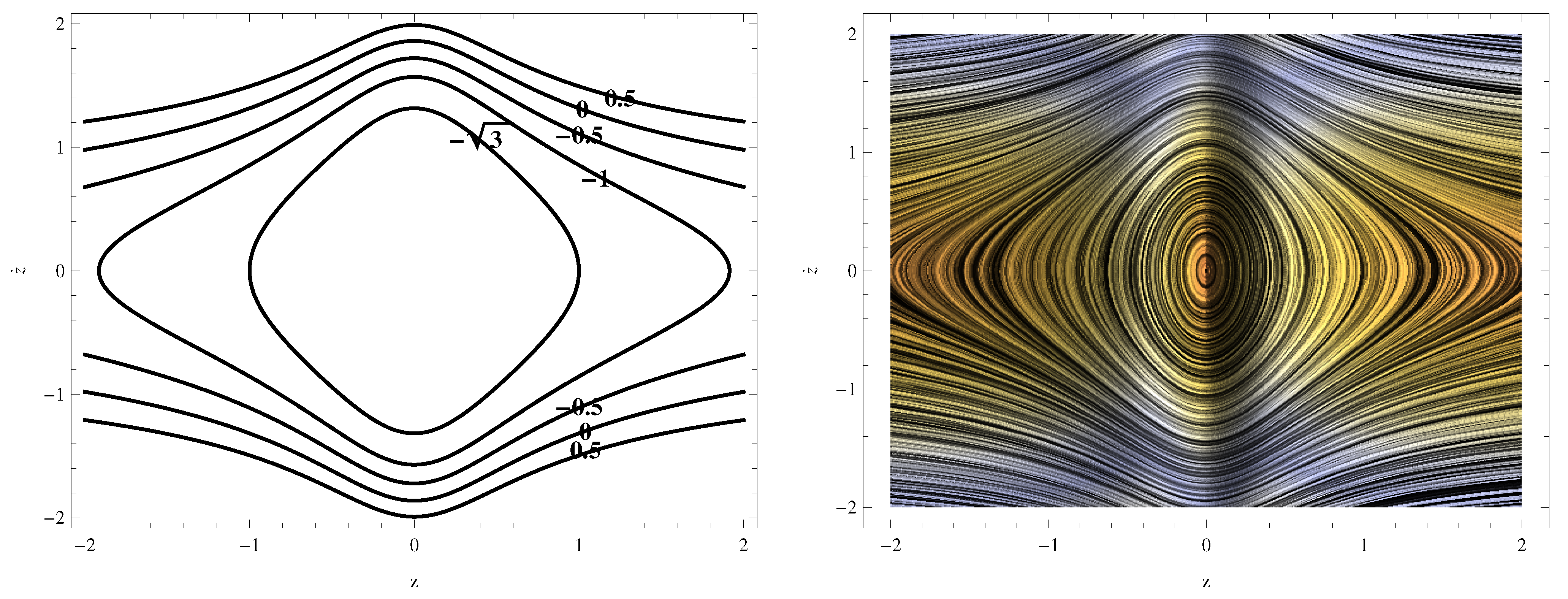
From
Figure 1, we can see that the potential function is symmetric at approximately
; hence, the potential function represents a harmonic oscillation motion.
In the Sitnikov problem, the motion of the infinitesimal body is described by a nonlinear differential equation given in Equation (
5). Moreover, in terms of elliptic functions, only the exact analytical solution can be derived and it is not possible in structures of mathematics. Hence, the alternative possible solutions are the approximated solutions which give the characteristics of the exact solution and are developed with the help of perturbation techniques. The perturbation techniques aim to obtain a solution of nonlinear differential equations with its own limitations. This depends on a parameter which is very small and does not appear in the equation of motion such that Equation (
1). The infinitesimal body moves with the Jacobian integral along the
z axis as its total energy which is given by
From (
1), we observed that when the potential is symmetric and close to the region
, then
that means the motion of the infinitesimal body is bounded in the interval
and the unbounded motions’ regions can be found when
. Moreover, the zero velocity of the infinitesimal body are in three cases. When it reaches infinity (
) with zero energy (
) in the first two cases, then there are two critical points at positive infinity as well as negative infinity. The motion is considered unbounded and the fourth body will stay stationary at infinity; whereas in the third case, the total energy takes the negative value
, i.e.,
and the fourth body moves to stay at the center of mass, i.e.,
, hence the motion is bounded and the fourth body also remains at the center of mass. It is observed that the from-zero velocity surfaces as well as the phase portrait are shown in
Figure 2.
The negative total energy means that the body has no ability to escape the gravitational pull of the central body. The negative total energy also means there is a certain position in which the kinetic energy will approximate towards zero. On the other hand, the negative energy does not mean that it is less than zero. It just implies that the orbiting body needs an amount of energy to be added, whether it comes to stable equilibrium or its own energy is zero [
25].
Since the total energy is close to
, hence it is negative and therefore, the fourth body will be close to the center of mass, thereby
. Therefore, with the help of Equation (
1), it is up to
obtained from:
where
and
.
With the help of the perturbation technique, the solution of the periodic motion of Equation (
9) is obtained. The term
appears in the equation as the perturbation term.
3. Solution by Lindstedt–Poincaré Method
When regular perturbation approaches fail to obtain periodic solutions in ordinary differential equations, a method is used which was developed by Anders Lindstedt (27 June 1854–16 May 1939) and Jules Henri Poincaré (29 April 1854–17 July 1912). Since
, we can then introduce a very small artificial parameter to the system which can be replaced by one in the final solution [
6]. In this case, we interchange the variable
z by
where
is very small (
); then, we can write
. Hence,
is also very small (
) where
is called the strength of the perturbation. Then, the equation of motion in second-order approximation: Equation (
9) can be rewritten as
A new independent variable
was introduced where
is an unspecified function of
, initially as a place-keeping parameter. The coefficient of the new governing equation of the second derivative contains
. This allows the amplitude and the frequency to interact, which is a property that is observed in nonlinear systems. The function
can be chosen in such a way as to eliminate the secular terms [
26].
Using
, Equation (
10) becomes:
Assuming the expansion for
as
where
are unknown constants. It is similar to straightforward expansion. The variable
z can be represented by an expansion having the form:
Substituting the values of Equations (
12) and (
13) into Equation (
11) and equating the coefficients of
and
to zero, we obtained the following differential equations:
For simple calculation, let us assume the initial conditions:
Utilizing conditions in Equation (
19) with Equation (
14), the solution of the first linear second-order initial value problem is given by
After utilizing Equations (
15) and (
20), then we obtain:
Now the first term on the right-hand side of Equation (
21) will lead to a secular term in the obtained solution; if the coefficient of
does not equal zero, then this coefficient must equal zero to avoid an unwanted term (secular term). Thus, we obtain:
hence, we obtain:
Therefore, Equation (
21) takes the form:
and its general solution is:
Applying the initial conditions
,
(
and
, satisfying our initial conditions) into Equation (
24), we obtain:
Hence, the final solution of Equation (
23) is:
Substituting the values of (
20), (
22) and (
26) into (
16), we obtain:
Again, the coefficient of
must be equal to zero to eliminate the secular term in
. This leads to:
Therefore, Equation (
27) reduces to:
and its general solution is:
With the help of initial conditions
,
(
and
, satisfying our initial conditions) in Equation (
30), we obtain:
Hence, the final solution of Equation (
29) is:
Substituting the values of (
20), (
22), (
24), (
28) and (
32) into (
17), we obtain:
Again, we have to put the coefficient of
equal to zero to eliminate the secular term in
. This means that:
Therefore, Equation (
33) reduces to:
and its general solution takes the form:
With the initial conditions
,
(
and
, satisfying our initial conditions) in Equation (
36), we obtain:
Hence, the final solution of Equation (
33) is:
Utilizing Equations (
20), (
22), (
24), (
28), (
32), (
34) and (
38) with Equation (
18), we obtain:
We have to put the coefficient of
equal to zero to eliminate the secular term in
. This means that:
Therefore, Equation (
39) is reduced to the form:
and its general solution is:
Using initial conditions
,
(
and
, satisfying our initial conditions) in Equation (
42), we obtain:
Hence, the final solution of Equation (
39) is:
Finally, substituting the values of
,
and
in Equation (
13) as well as
and
in Equation (
12), we obtain:
with:
Equations (
45) and (
46) are the desired solutions up to fourth-order approximation of the system, while all terms with order
and higher are ignored. At the end, the parameter
can be replaced by one for obtaining the final form solution according to the place-keeping parameters method.
4. Numerical Results
A comparison was carried out among the numerical: the first-, second-, third- and the fourth-order approximated solutions in the Sitnikov RFBP. The investigation includes the numerical solution of Equation (
5) and the first, second, third and fourth-order approximated solutions of Equation (
10) obtained using the Lindstedt–Poincaré method which are given in Equations (
45) and (
46), respectively.
The comparison of the solution obtained from the first-, second-, third- and fourth-order approximation with a numerical solution obtained from (
1) is shown in
Figure 3,
Figure 4 and
Figure 5, respectively. We take three different initial conditions to make the comparison. The infinitesimal body starts its motion with zero velocity in general, i.e.,
and at different positions (
,
,
).
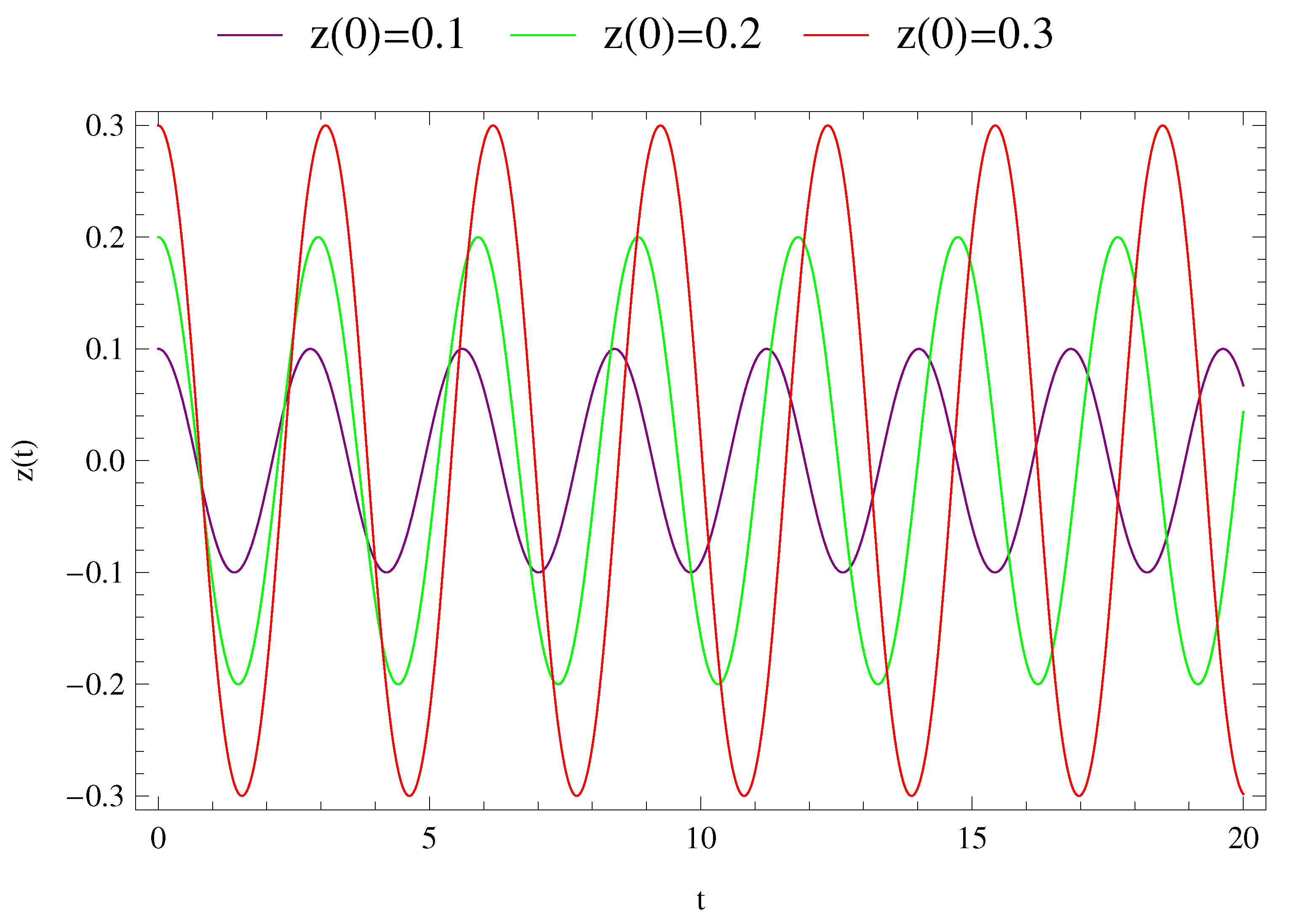
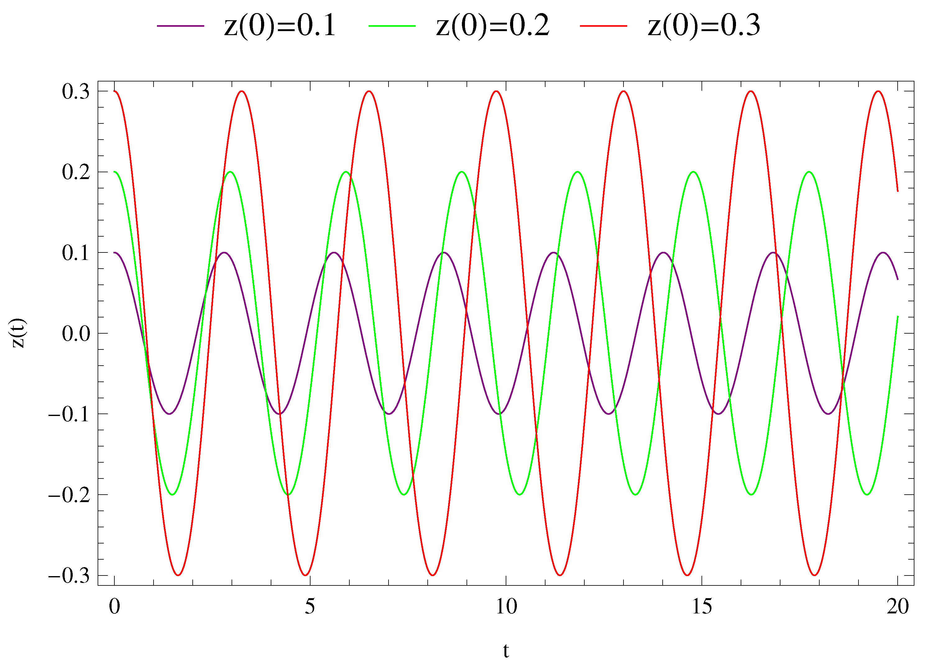
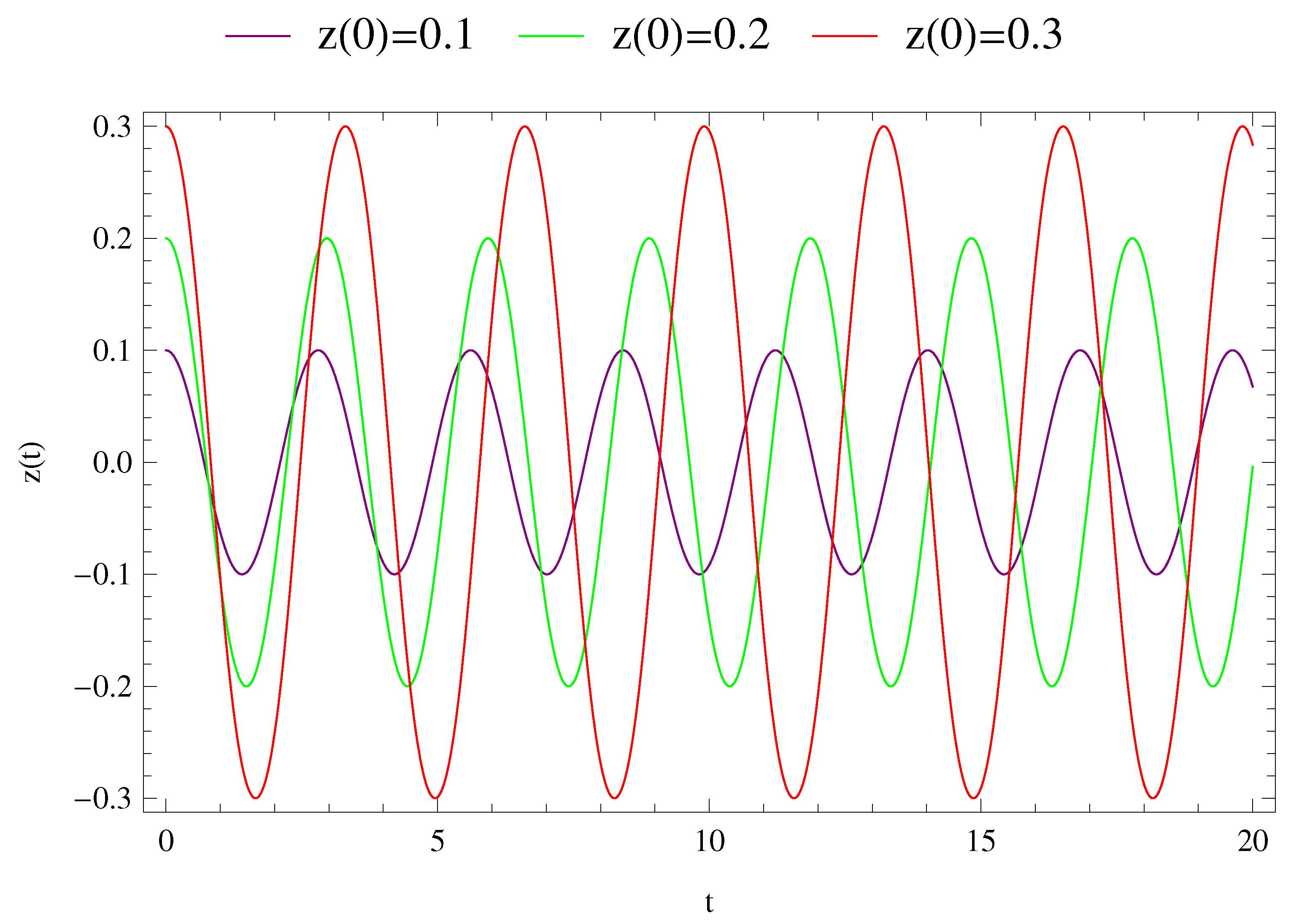
The investigation of motion of the infinitesimal body was divided into two groups. In a first group, three different solutions were obtained for three different initial conditions, which are shown in
Figure 6,
Figure 7,
Figure 8,
Figure 9 and
Figure 10. In these figures, the purple, green and red curves refer to the initial condition
,
and
, respectively. However, in a second group, three different solutions were obtained for the above given initial conditions. This group includes
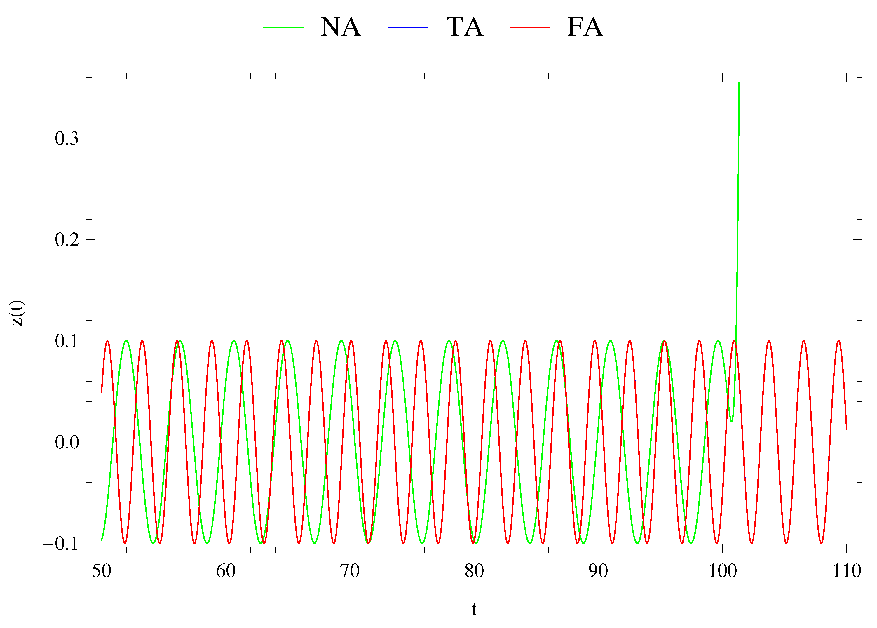
Figure 3,
Figure 4 and
Figure 5, in which the green, blue and red curves indicate the numerical solution (NA), third-order approximated (TA) and fourth-order approximations (FA) of the Lindstedt–Poincaré method, respectively, in these figures.
In
Figure 10, we see that the motion of the infinitesimal body is periodic, and its amplitude decreases when the infinitesimal body begins moving closer to the center of mass. Moreover, in numerical simulation, the behavior of the solution is changed by the different initial conditions. Furthermore, the numerical solution is not bounded (we mean that the motion is not periodic) to the infinitesimal body which begins its motion from a large distance to the center of mass of the primaries. Perhaps, the solution has periodic behavior with regular periodicity for the proper selection of initial conditions during a certain time period.
From
Figure 3,
Figure 4 and
Figure 5, we impose that the infinitesimal (fourth-) body starts moving from three different position with respect the center of mass of primaries. Motion is periodic in the interval
and its amplitude decreases when its motion starts nearer to the position because of the common center of masses of the primaries, which agree with [
6]. On the other hand, when
, the numerically obtained motion is then periodic, however, when
, it escapes from the path of the orbit.
5. Conclusions
In this paper, the periodic solutions of the Sitnikov restricted four-body problem (RFBP) were constructed by using the Lindstedt–Poincaré method by removing the unbounded terms, which are called the secular. These solutions are compared with numerical solution to verify the importance of the used perturbation method (Lindstedt–Poincaré method). One of the major significant aims of removing secular terms is determining the conditions which enforce the motion to be periodic or establish the periodicity conditions of motion. Under these conditions, we can find approximated periodic solutions in closed form. It was observed that in the numerical and the obtained periodic solutions’ patterns, the initial conditions are very important. The motion was numerically examined and compared with the approximated solution obtained by the Lindstedt–Poincaré method.
We remark that the motion is periodic in the time interval ; however, beyond this interval, the motion is not periodic in the numerical sense. However, the Lindstedt–Poincaré method gives regular and periodic motion for a time of . In addition, we note that the motion obtained by the first-, second-, third- and fourth-order approximate solutions is regular and periodic when the test particle starts its motion closer to the center of the mass. On the other hand, the test particle starts its motion far from the center of mass and the solutions obtained by numerical simulation may not be periodic for a long time—whereas all the first- to fourth-order approximated solutions may become regular and periodic motions. We demonstrated that the obtained solution by the Lindstedt–Poincaré method gives the true motion of the circular Sitnikov RFBP and the fourth-order approximate solution has more accuracy than the first-, second- and third-order approximate solutions.
In the future study, we aimed to present more analysis of the dynamical motion of the body problem, particularly the circular and elliptical Sitnikov motion. In this context, we will use some power tools to find periodic solutions such as the method of parameter variation and averaging or the multiple scales technique, which is considered a generalization of the Lindstedt–Poincaré method.


