Abstract
The all-at-once technique has attracted many researchers’ interest in recent years. In this paper, we combine this technique with a classical symplectic and symmetric method for solving Hamiltonian systems. The solutions at all time steps are obtained at one-shot. In order to reduce the computational cost of solving the all-at-once system, a fast algorithm is designed. Numerical experiments of Hamiltonian systems with degrees of freedom are provided to show that our method is more efficient than the classical symplectic method.
1. Introduction
Hamiltonian mechanics, along with Newtonian mechanics and Lagrangian mechanics, are three classical mechanics. It is a reformulation of the classic mechanics that evolved from Lagrangian mechanics. The Hamiltonian system is developed based on Hamiltonian mechanics. The Hamiltonian system is an important category of dynamical systems, which can represent all real physical processes with negligible dissipation. It has a very wide range of applications, such as biology [1], plasma physics [2,3,4,5] and celestial mechanics [6,7]. The basis of Hamiltonian system is symplectic geometry which is the phase space composed of n generalized coordinates and n generalized momentum in a system with n degrees of freedom. The remarkable property of a Hamiltonian system is that it has intrinsic symplectic structure which is preserved by its phase flow.
It is usually difficult to obtain the phase flow of a Hamiltonian system, even though it preserves the certain symplectic structure. Therefore, the numerical method that may preserve the symplectic structure of the Hamiltonian system is an alternative choice. Thus, the symplectic method [8] is developed to numerically simulate the Hamiltonian system, aiming to preserve the symplectic structure. Its structure-preservation property and symplectic method have a great advantage in computational stability and long-term simulation over conventional numerical schemes. Such an advantage afford the symplectic algorithm tremendous success in diverse areas, e.g., mechanics, biology and physics [1,4,7,9,10,11,12,13]. Particularly, symplectic algorithms have been widely applied in plasma physics in recent years. The charged particle dynamics and guiding center dynamics in electro-magnetic fields can be expressed as a Hamiltonian system and a non-canonical Hamiltonian system, respectively. Explicit sympletic methods based on generating functions and coordinate transformations are developed for charged particle dynamics [5,13]. For guiding center dynamics of charged particles, variational symplectic methods [2,14] and canonicalized symplectic method [4] have been proposed.
Traditionally, the symplectic method is a time-stepping scheme, which obtains the solutions step-by-step. The symplectic method is usually implicit, thus an iteration method, such as fixed point iteration method or Newton iteration method is needed to solve the method. If a large number of time steps are involved, the total number of iterations can be very large, and the symplectic method may become time-consuming. Therefore, to overcome the time-consuming problem of the time-stepping method, we propose an alternative method. The basic idea of our method is combining the all-at-once technique with a sympletic method. For convenience, we call this novel method the symplectic all-at-once method in this paper. More precisely, we stack the solutions of the symplectic method at all time steps in a vector, then an all-at-once system or a block lower triangular system will be obtained. Such a lower triangular structure facilitates the use of the fast algorithm. We will show in the numerical experiments that our method equipped with a fast algorithm takes less computational cost than the time-stepping method.
More and more researchers have paid attention to the all-at-once technique in recent years as it can obtain the solution at all time steps. The all-at-once method has been widely used in time-dependent optimal control problems [15,16] and fractional partial differential equations (FPDEs) [17,18,19,20,21,22]. Stoll and Wathen [15] used the all-at-once approach to solve the discretized unsteady Stokes problems. This approach was shown to be efficient and mesh-independent. The all-at-once method was also applied for the optimal control of the unsteady Burgers equation [16]. Furthermore, the all-at-once technique equipped with fast algorithms was utilized when using finite difference methods to solve FPDEs [17,18,19,20,21,22]. The reason why many researchers use the all-at-once approach is to reduce the computational cost. Zhao et al. [20] employed the all-at-once approach for the time–space fractional diffusion equation. They developed a block bi-diagonal Toeplitz preconditioner for efficiently solving their resulting system. Gu and Wu proposed a parallel-in-time iterative algorithm for solving the all-at-once system arising from partial integro-differential problems [17]. The fast implementations for solving block lower triangular systems arising from fractional differential equations can be found in [18,19] and the references therein.
In this paper, we develop a sympletic all-at-once method for Hamiltonian systems. The all-at-once system is solved by the Newton method equipped with a fast algorithm which greatly saves computational time. Numerical experiments in three Hamiltonian problems are carried out to show that our method is more efficient than the classical symplectic method.
The rest of this paper is organized as follows. In Section 2, we first give a review of symplectic methods for Hamiltonian systems. Then, we derive the all-at-once system based on the midpoint rule. Accordingly, we provide a framework of our method for solving Hamiltonian systems. In Section 3, several numerical examples are provided to show the performance of our method. Moreover, we also compare our method with the classical midpoint rule and the third order non-symplectic Runge–Kutta method. In this paper, we only conduct experiments on Hamiltonian systems with degrees of freedom . In Section 4, we summarize our work and make enlightening remarks.
2. All-at-Once System for Hamiltonian Systems
Firstly, we give a short introduction to Hamiltonian systems and symplectic methods.
2.1. Symplectic Methods for Hamiltonian Systems
It is well known that the Hamiltonian system [1,7,11] is an important category in ordinary differential equations. Hamiltonian systems exist in diverse areas of physics, mechanics and engineering. It is generally accepted that all the physical process with negligible dissipation may be expressed as suitable Hamiltonian systems. So, reliable numerical methods that are developed for the numerical solution of Hamiltonian system would have wide applications. A prominent property of Hamiltonian systems is the symplecticity of the phase flow. Therefore, symplectic method is developed to preserve the symplectic structure of the Hamiltonian system.
In this paper, we consider the autonomous Hamiltonian system
where is the Hamiltonian function and and represent the momentum and configuration variables, respectively. If we combine all the variables in (1) in a dimensional vector , then (1) takes the compact form
where J is a skew-symmetric matrix
with and 0 representing the identity and zero matrix, respectively. By differentiating H with respect to t along the solution of system, we find that
Then, Hamiltonian function H is a conserved quantity which remains constant along the solution of the system. It is also called the energy of the system.
It is worth mentioning that in this paper, we only consider the autonomous Hamiltonian system (1). For non-autonomous Hamiltonian systems, we can trasform them to autonomous ones [10]. More precisely, for the following non-autonomous Hamiltonian system
with momentum variables and conjugate variables , it can be transformed to an autonomous Hamiltonian system by adding a conjugate pair . This approach is to consider the time t as an additional conjugate variable. The new momentum h, to interpret it physically, is the negative of the total energy. Then the corresponding phase space has dimension, , and the new Hamiltonian function . Accordingly, the system becomes
It is an autonomous Hamiltonian system
with Hamiltonian function .
As is mentioned above, the symplecticity of the phase flow is a characteristic of Hamiltonian systems. That means that the phase flow of the Hamiltonian system (2) preserves symplectic structure, i.e., satisfies
In most occasions, it is difficult to obtain the exact solution of (2) when the system is highly nonlinear. So, we resort to using numerical methods to solve (2), such as the symplectic geometric methods [1,7,8,11].
Definition 1.
A numerical method
is called symplectic if it satisfies
for a given time stepsize τ.
Notice that the symplectic method still preserves the symplectic structure, just as the phase flow of Hamiltonian systems does. Furthermore, the symplectic method possesses another important property: long-term energy conservation.
Among all kinds of symplectic methods, symplectic Runge–Kutta method [1,11] is a commonly used method because of its stability. An stage Runge–Kutta method is given by
where and are real numbers, is the time stepsize and is the forward value of the variable y based on the known value .
Theorem 1.
A Runge–Kutta method is symplectic if the coefficients satisfy [23,24]
Generally, an explicit Runge–Kutta method does not satisfy the above symplectic condition. Thus, a symplectic Runge–Kutta method is usually implicit. Midpoint rule [1,7,11] is a second order one-stage symplectic Runge–Kutta method. Formally, we take the midpoint rule as
Definition 2.
A numerical method
is said to be symmetric if it satisfies
The above condition has an equivalent expression [1].
To obtain the adjoint method from , we just need to exchange and . By comparing the midpoint rule with its adjoint method, we find that they are exactly the same. Thus, the midpoint rule is a symmetric method. The midpoint rule is widely used for simulating Hamiltonian systems because of its symmetry and stability [4,25,26]. In our work, the all-at-once technique based on the midpoint rule is derived for solving (2).
2.2. All-at-Once System
We assume that the ordinary differential Equation (ODE) is of particular form
The case that f includes a slow explicit dependence on t, i.e., , may be trivially reduced to (5) by adding a component to the state vector y and setting . If the ODE system is a Hamiltonian system, then the case is a non-autonomous Hamiltonian system. According to the preceding section, by adding a conjugate pair, the non-autonomous system can be transformed to an autonomous one. Thus, the case (5) we considered is of generality. To simulate the solutions of general ODEs, the traditional way is to proceed the solution step-by-step, i.e., the so called time-stepping method. The all-at-once method stacks the solutions at all time steps in a vector, which proceeds all the solutions simultaneously by solving the resulted all-at-once system.
By applying the all-at-once technique to the midpoint rule, a bi-diagonal block structure will be obtained, which greatly reduces the storage requirement. Precisely, let us take N time steps with , then the time discretization of the ODE system is
where . Then, we can construct the following nonlinear system with the solutions at all time steps:
where and . This bi-diagonal block structure makes the fast computation possible. Aiming to solve this nonlinear system, the Newton iteration method is chosen in this article. It is well known that the Newton method has the property of second-order convergence, thus less iteration is required to obtain the satisfactory solution than other iteration methods. Therefore, the Newton method is suitable to solve the all-at-once system. In order to proceed the Newton method, the initial value and the Jacobian matrix in each iterative step are required. Therefore, a well-chosen initial value and an efficient method to solve the Jacobian equations are two essential ingredients to solve (6).
Here is the stratergy: We solve (6) on a coarse mesh based on using higher order symplectic methods. Then, we use the interpolate method to obtain the initial value on a fine mesh. More precisely,
Step 1: Let () be the large time stepsize and the time steps . Using the fourth order Gauss’ method [1,11] to integrate the Hamiltonian system (2) aiming at calculating the values .
Step 2: Using the interpolation method, such as the piecewise cubic Hermite interpolating polynomial, to obtain the initial value .
The expression of fourth order Gauss’ method is
It is a symplectic and symmetric Runge–Kutta method. Gauss’ method is used to calculate the datum on the coarse mesh. As symplectic method preserves the symplectic structure of Hamiltonian systems, Gauss’ method can obtain more favorable results than other non-symplectic methods under large time stepsize . The value of is often determined by the experimental result. In fact, the chosen of influences not only the total computational time, but also the initial value of the Newton method. The convergence speed of the Newton method is highly affected by the initial value. Newton method converges fast if a good initial value is chosen. Furthermore, the initial value is generated by using a numerical method to calculate the values on a coarse mesh under big time stepsize , then interpolating the values on a fine mesh under small stepsize. If or a numerical method is not properly chosen, then the initial value obtained by using interpolation method is not good enough, as a result, the Newton method will converge very slow, the computational cost will be very high. Therefore, a suitable value of and a high order method with good property such as the fourth order Gauss’ method are two important ingredients for generating the initial value of the Newton method.
For the second problem, we rewrite Equation (6) as follows
Then, we calculate the Jacobian matrix of . Note that depends only on and , thus the Jacobian matrix is
where and . It can be seen that is a lower bi-diagonal block matrix which facilitates the use of fast algorithm to compute its inverse. The essential part of the Newton method is how to compute as fast as possible, where v is a vector with a suitable size. Here, we use block Thomas method (see Algorithm 1). In fact, due to the bi-diagonal block structure of , the vector can be divided into N blocks and every block is a d dimensional vector. Thus, we can derive every block iteratively. The vector v is divided into N blocks as well. Then, the first block of is equivalent to multiplying the first block of v. Furthermore, the second to the N-th block of can be derived iteratively. Thus, according to Algorithm 1, we can easily obtain the vector , which accelerates the process of the Newton iteration.
| Algorithm 1 Compute |
|
In this paper, we apply an all-at-once technique to the midpoint rule for Hamiltonian systems. We only consider the Hamiltonian system (2) with degrees of freedom ( dimension), the cases with will be considered in our future work. When or 2, the inverse of , in lines 2 and 5 of Algorithm 1 can be calculated directly. Thus, only memory is needed in Algorithm 1 and the computational complexity of this algorithm is . For , the computation of may not be fast, then in Algorithm 1 we may use Krylov subspace method [27] to compute . The Krylov subspace method is very efficient to compute . An advantage of this method is that it avoids directly calculating the inverse of A.
Remark 1.
If the integration time is very long, we need to make a further partition of the time interval into several subintervals for the all-at-once system.
3. Numerical Experiments
All experiments were performed in MATLAB R2016b on a Windows 10 (64 bit) PC with the configuration: Intel(R) Core(TM) i7-8550U CPU 1.80 GHz and 16 GB RAM. The methods we used to perform numerical simulation are listed as follows.
AAO: symplectic all-at-once method which is a combination of all-at-once technique with the midpoint rule. Newton iteration method equipped with Thomas algorithm is utilized to solve the obtained all-at-once system. The midpoint rule is a second order symmetric and symplectic method.
TS: time-stepping method which represents the traditional way to deal with the midpoint rule. The solutions are obtained step-by-step.
RK3: the third-order Runge–Kutta method [4] which is neither sympletic nor symmetric. The method can be expressed as
3.1. Example 1: Harmonic Oscillator
First, we consider the well-know Hamiltonian system with one degree of freedom
Here, q represents the configuration variable and p is the momentum. This system describes the motion of a particle of mass m attached to a spring with stiffness constant k. Here, T and V are kinetic energy and potential energy, respectively, [11].
As the harmonic oscillator is a Hamiltonian system, the equations can be written as
When we plot the phase plane , the curves are ellipses
If , the curves are circles.
The simple harmonic oscillators constitute a Hamiltonian system with the conjugate variables . We consider the case for and , then the Hamiltonian system reads
with [11]. The exact solution is
We first integrated the problem (8) with the symplectic all-at-once method under the initial condition , . The Newton iteration method for solving (6) terminates if the tolerance error is less than or the iteration number is more than 2000. The coarse time stepsize for the symplectic all-at-once method is . Then we integrated the problem (8) with the time-stepping method and third order Runge–Kutta method.
Firstly we compare the symplectic all-at-once method with the third order Runge–Kutta method. We have displayed in Figure 1 the phase orbits and the energy errors of both methods over the interval [0, 20,000]. The phase orbit of the symplectic all-at-once method is accurate over a long time, but the phase orbit of the third order Runge–Kutta method spirals inwards over time. The energy error of the symplectic all-at-once method is preserved very well, but that of the the third order Runge–Kutta method increases over time. Therefore, the symplectic all-at-once method has significant advantage in preserving the phase orbit and the energy of the system over the third order Runge–Kutta method. The reason why the symplectic all-at-once method behaves better than the third order Runge–Kutta method is that the midpoint rule is symmetric and symplectic.
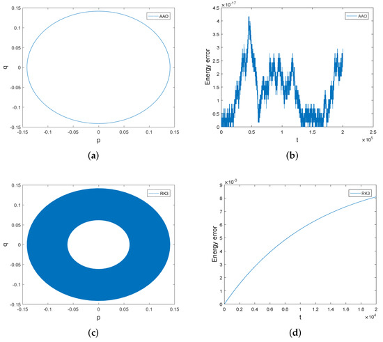
Figure 1.
The phase orbits and the energy errors of the symplectic all-at-once method and third order Runge–Kutta method over the interval [0, 20,000]. The stepsize . Subfigure (a,b) are the phase orbit and energy error obtained by symplectic all-at-once method. Subfigure (c,d) are the phase orbit and energy error of third order Runge-Kutta method.
Then, we compare the computational efficiency of the symplectic all-at-once method and the time-stepping method. Table 1 reports, for varying time stepsize , the CPU times of the symplectic all-at-once method and the time-stepping method, over the interval . By looking at the columns of Table 1, we find that solving the all-at-once system is a bit faster than solving the system (8) using the time-stepping method. When the stepsize is or , the CPU time of the time-stepping method is nearly twice of that of the symplectic all-at-once method. The global errors of p and q of the symplectic all-at-once method are displayed in Table 1. Figure 2 indicates that the global error behaves as which clearly shows the order of the midpoint rule. We have displayed in Table 2 the global errors of p and q of the time-stepping method and they are the same as those of the symplectic all-at-once method. The discrepancy between the solutions computed by both methods is also presented in Table 2. The maximum errors under different stepsizes are less than the value .

Table 1.
The CPU times of the symplectic all-at-once method (AAO) and the time-stepping method (TS) and global error of the symplectic all-at-once method over the time interval .
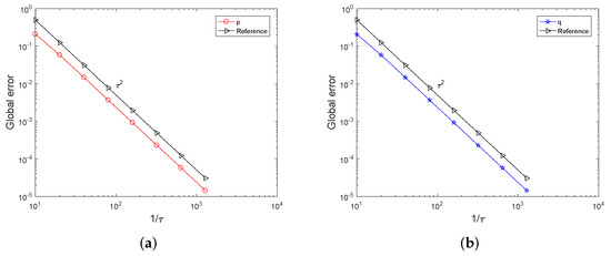
Figure 2.
The global errors of p and q over the interval . Subfigure (a) presents the global error of p of symplectic all-at-once method while Subfigure (b) presents the global error of q. Both subfigures clearly show the order of symplectic all-at-once method is 2.
Table 2.
The global errors of p and q of the time-stepping method (TS) and the maximum errors of p and q between the symplectic all-at-once method and the time-stepping method over the time interval .
We have also integrated the system over long time interval [0, 20,000] and the comparison results are displayed in Table 3. At all time stepsizes, the CPU times of the symplectic all-at-once method are less than those of the time-stepping method. The difference in CPU time becomes larger when the stepsize turns smaller. The maximum energy errors between the two methods at all stepsizes are very close to the machine accuracy. In conclusion, the symplectic all-at-once method is more efficient than the time-stepping method.
Table 3.
The comparison of CPU times and maximum energy errors (in the variable p) between the symplectic all-at-once method (AAO) and the time-stepping method (TS) over the interval [0, 20,000].
3.2. Example 2: Hénon–Hiles Model
The Hénon–Hiles Model describes stellar motion in celestial mechanics [1,28]. More precisely, it describes the star’s motion under the action of a gravitational potential of a galaxy with cylindrical symmetry. Hénon and Hiles reduced the dimension of the system, and they show that the model actually describes the motion of a particle in a plane with the total energy [1,28]
where the potential function is arbitrary. They chose the potential as
When the potential energy approaches , the level curves of tends to an equivalent triangle and the triangle finally forms the region
If one choose a starting point such that the total energy
then the solution stays in the region R. However, if one choose a starting point that the energy H approaches , the chaotic behavior will occur.
We have displayed in Figure 3 that the Poincare section [1,11] of with the plane obtained by the symplectic all-at-once method. Figure 3a shows a quasi-periodic solution with the initial energy . The initial condition is . Figure 3b shows a chaotic solution with the initial energy . The initial condition is . The intersections depicted in Figure 3a correspond to one trajectory; they lie on a curve which indicates the quasi-periodic behavior. We can see from Figure 3b that the intersections do not stay in a curve, but are scattered in the two-dimensional plane. This trajectory is called chaotic. The energy errors of the symplectic all-at-once method for the quasi-periodic trajectory and the chaotic trajectory are also displayed in Figure 3c,d. Energy error is presented by . In both cases, the energy error is bounded by a very small interval. Thus, the symplectic all-at-once method can not only accurately depict the chaotic motion, but also nearly preserves the energy over long time.
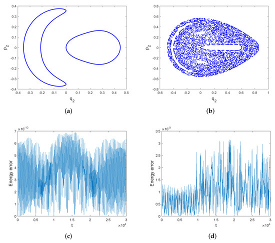
Figure 3.
Subfigure (a) shows the Poincare section of with the plane. The initial energy is . The integration is performed by the symplectic all-at-once method for 30,000 with stepsize . Subfigure (b) shows the Poincare section of with the plane. The initial energy is . The integration is performed by the symplectic all-at-once method for 30,000 with stepsize . Subfigure (c,d) show the energy errors of the symplectic all-at-once method for both trajectories.
We choose the total energy as above , then the Hénon–Hiles model can be expressed as a four dimensional Hamiltonian system [1,28]
We integrated the system (9) with the symplectic all-at-once method and the time-stepping method over the time interval [0, 10,000]. The initial condition is chosen as , such that . The coarse time stepsize for the symplectic all-at-once method is .
The Poincare section of with the plane and the energy errors of the symplectic all-at-once system and the third order Runge–Kutta method are shown in Figure 4. The Poincare sections of both methods do not show much difference. However, the symplectic all-at-once method behaves better in energy conservation than the third order Runge–Kutta method. We can see from Figure 4 that the energy error of the symplectic all-at-once method is bounded by a very small number, but that of the third order Runge–Kutta method increases without bound.
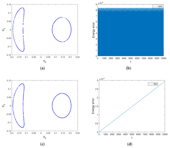
Figure 4.
The Poincare section of and energy errors of symplectic all-at-once method and third order Runge–Kutta method over the interval [0, 10,000]. The stepsize is . Subfigure (a,b) display the Poincare section and energy error of symplectic all-at-once method, while Subfigure (c,d) display the Poincare section and energy error of third order Runge-Kutta method.
We report in Table 4 for the global errors of and of the symplectic all-at-once method under different time stepsize over the interval . It can be seen that the convergence order of the symplectic all-at-once method is nearly 2. This clearly shows that the symplectic all-at-once method is of order 2. The global errors of the time-stepping method under different stepsizes are displayed in Table 5, and they are the same as those of the symplectic all-at-once method. The maximum errors of and between two methods are also presented in Table 5. We can see that the errors are of small value (less than ).
Table 4.
The global errors of variables and of the symplectic all-at-once method (AAO) over the interval .
Table 5.
The global errors of variables and of the time-stepping method (TS) and the maximum errors of and between the symplectic all-at-once method and the time-stepping method over the interval .
Furthermore, the CPU times of the symplectic all-at-once method and the time-stepping method for varying are reported in Table 6. From the table, we see that the CPU times of the symplectic all-at-once method are less than those of the time-stepping method. The advantage of the symplectic all-at-once method in CPU time becomes more obvious when is smaller. This clearly shows that the symplectic all-at-once method is more efficient than the time-stepping method. The maximum energy errors between the two methods are also presented in Table 6. The energy errors approximately reach the machine accuracy.
Table 6.
The comparison of CPU times and maximum energy errors between the symplectic all-at-once method (AAO) and the time-stepping method (TS) over the interval [0, 10,000].
3.3. Example 3: Charged Particle System
Theoretically, there are three methods to describe the motion of plasma while the single charged particle motion is the simplest one. We describe the motion of one single charged particle in given electro-magnetic field without taking account of the reaction of the charged particle motion to the field and the interactions between charged particles. The motion of charged particles is the most fundamental equation and it helps people have a better understanding of many important phenomena in plasma physics research. The dynamics of one single charged particle in a magnetized plasma is a multi-scale problem because it contains two components: the fast gyromotion and the slow guiding center motion. On one hand, by averaging out the fast gyromotion, the guiding center motion can be obtained. The behaviour of guiding centers is governed by gyrokinetics and related theories. On the other hand, by rewriting the equations of the single charged particle motion, it is found that the motion can be expressed as a Hamiltonian system if the Cartesian coordinate is chosen. Here, the variable is the configuration variable and is the momentum.
The dynamics of a charged particle with the Lorentz force [3,5,13] in the coordinate is
which can be written as a Hamiltonian system
where is a six-dimensional vector and the Hamiltonian function . Here are constants, is the vector potential. The relation of the magnetic field and the vector potential is . We integrated the system (10) with the symplectic all-at-once method and the time-stepping method over the time interval . The initial condition for the position variables is and the velocity is . The vector potential is chosen to be .
The global errors of variables x and of the symplectic all-at-once method under different time stepsize over the interval are displayed in Table 7. The global errors computed by the symplectic all-at-once method in Table 7 and those computed by the time-stepping method in Table 8 are the same. It is shown in Table 7 the convergence order of the symplectic all-at-once method is 2 which means that the method is of order 2. We have also computed the maximum errors of x and between two methods, they are all of very small value (less than ). The maximum errors nearly reach the machine accuracy.
Table 7.
The global errors of variables x and of the symplectic all-at-once method (AAO) over the interval .
Table 8.
The global errors of variables x and of the time-stepping method (TS) and the maximum errors of x and between the symplectic all-at-once method and time-stepping method over the interval .
We first compare the phase orbits and the energy errors of the symplectic all-at-once method and the third order Runge–Kutta method. Displayed in Figure 5 are the orbits of two components of and the energy errors of both methods over the interval . We can see that the orbit of the symplectic all-at-once method is very accurate over long time, but the orbit of the third order Runge–Kutta method spirals inward over time. The energy error of the symplectic all-at-once method is bounded by a very small number, while the energy error of the third order Runge–Kutta method is not bounded and increase along time. The energy errors of the third order Runge–Kutta method are much larger than those of the symplectic all-at-once method. Therefore, the symplectic all-at-once method has overwhelming advantage in tracking the orbit and preserving the energy than the third order Runge–Kutta method.
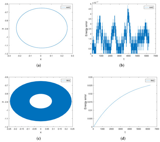
Figure 5.
The orbits of and the energy errors of the symplectic all-at-once method and the third order Runge–Kutta method over the interval . The stepsize . Subfigure (a,b) present the orbit of and energy error of symplectic all-at-once method, while Subfigure (c,d) present the orbit of and energy error of third order Runge-Kutta method.
Table 9 reports the CPU times of the symplectic all-at-once method and the time-stepping method over the interval with different stepsizes . We can see from Table 9 that the CPU times of the symplectic all-at-once method are all less than those of the time-stepping method. Especially, when the stepsize is less than , the CPU time of the time-stepping method is three times of that of the symplectic all-at-once method. Therefore, this clearly shows that the symplectic all-at-once method is more efficient than the time-stepping method. We have also reported the Newton iteration of the symplectic all-at-once method and the iterations are all 3, which shows the efficiency of our method.
Table 9.
The comparison of CPU times between the symplectic all-at-once method (AAO) and the time-stepping method (TS) over the interval .
4. Conclusions
We have proposed a symplectic all-at-once method to integrate Hamiltonian systems. The symplectic all-at-once method is a combination of the all-at-once technique and the symplectic midpoint rule. When applying the all-at-once technique to the midpoint rule, we obtain a lower bi-diagonal block system. This bi-diagonal block structure facilitates the use of the fast algorithm. The Newton method equipped with Thomas algorithm are used to rapidly solve this system. The numerical results of the three Hamiltonian problems show that our method is more efficient than the time-stepping method. It is also shown that our method has a significant advantange in tracking the phase orbit and preserving the energy of the system compared to the third order non-symplectic Runge–Kutta method. Thus, the symplectic all-at-once method provides a good choice for solving the Hamiltonian system (2).
In this work, we only consider dimensional Hamiltonian systems with . For or 2, the inverse of , in lines 2 and 5 of Algorithm 1 can be calculated directly. Thus, the computational complexity is highly reduced. For , we suggest using Krylov subspace methods to perform fast computation because the Krylov subspace method does not need to compute in Algorithm 1. We only consider the combination of the all-at-once technique and symplectic methods. Apart from symplectic methods, volume-preserving methods and energy-preserving methods are also two important categories of structure-preserving algorithms. They can preserve one of the invariant of Hamiltonian system, the volume and the energy of the system, respectively. Thus, they are also good numerical methods to simulate the Hamiltonian system. In the future work, we will consider combining the all-at-once technique with energy-preserving methods and volume-preserving methods, and then designing fast algorithms for these all-at-once systems.
Author Contributions
Conceptualization, B.-B.Z., Y.-L.Z.; Formal Analysis, Y.-L.Z.; Funding acquisition, B.-B.Z.; Methodology, B.-B.Z., Y.-L.Z.; Software, B.-B.Z.; Writing—original draft, B.-B.Z. All authors have read and agreed to the published version of the manuscript.
Funding
This research was funded by the National Natural Science Foundation of China (Grant No. 11901564).
Conflicts of Interest
The authors declare no conflict of interest.
Abbreviations
The following abbreviations are used in this manuscript:
| AAO | All-at-once |
| TS | Time-stepping |
References
- Hairer, E.; Lubich, C.; Wanner, G. Geometric Numerical Integration: Structure-Preserving Algorithms for Ordinary Differential Equations; Springer: Berlin/Heidelberg, Germany, 2002. [Google Scholar]
- Qin, H.; Guan, X. Variational symplectic integrator for long-time simulations of the guiding-center motion of charged particles in general magnetic fields. Phys. Rev. Lett. 2008, 100, 035006. [Google Scholar] [CrossRef] [Green Version]
- Tu, X.B.; Zhu, B.B.; Tang, Y.F.; Qin, H.; Liu, J.; Zhang, R.L. A family of new explicit, revertible, volume-preserving numerical schemes for the system of Lorentz force. Phys. Plasma 2016, 23, 122514. [Google Scholar] [CrossRef]
- Zhang, R.L.; Liu, J.; Tang, Y.F.; Qin, H.; Xiao, J.Y.; Zhu, B.B. Canonailization and symplectic simulation of the gyrocenter dynamics in time-independent magnetic fields. Phys. Plasma 2014, 21, 03504. [Google Scholar]
- Zhou, Z.Q.; He, Y.; Sun, Y.J.; Liu, J.; Qin, H. Explicit symplectic methods for solving charged particle trajectories. Phys. Plasma 2017, 24, 052507. [Google Scholar] [CrossRef]
- Emel’yanenko, V.V. A method of symplectic integrations with adaptive time-steps for individual Hamiltonians in the planetary N-body problem. Celest. Mech. Dyn. Astr. 2007, 98, 191–202. [Google Scholar] [CrossRef]
- Feng, K. Collected Works of Feng Kang: II; National Dence Industry Press: Beijing, China, 1995. [Google Scholar]
- Feng, K. On difference schemes and symplectic geometry. In International Symposium on Differential Geometry and Differential Equations; Science Press: Beijing, China, 1984; pp. 42–58. [Google Scholar]
- Channell, P.J.; Scovel, J.C. Symplectic integration of Hamiltonian systems. Nonlinearity 1990, 3, 231–259. [Google Scholar] [CrossRef]
- Feng, K.; Qin, M.Z. Symplectic Geometric Algorithms for Hamiltonian System; Springer: New York, NY, USA, 2009. [Google Scholar]
- Sanz-Serna, J.M.; Calvo, M.P. Numerical Hamiltonian Problems; Chapman and Hall: London, UK, 1994. [Google Scholar]
- Tang, Y.F. Formal energy of a symplectic scheme for Hamiltonian systems and its applications (I). Comput. Math. Appl. 1994, 27, 31–39. [Google Scholar]
- Zhang, R.L.; Qin, H.; Tang, Y.F.; Liu, J.; He, Y.; Xiao, J.Y. Explicit symplectic algorithms based on generating functions for charged particle dynamics. Phys. Rev. E 2016, 94, 013205. [Google Scholar] [CrossRef] [Green Version]
- Qin, H.; Guan, X.; Tang, W.M. Variational symplectic algorithm for guiding center dynamics and its application in tokamak geometry. Phys. Plasmas 2009, 16, 042510. [Google Scholar] [CrossRef]
- Stoll, M.; Wathen, A. All-at-once solution of time-dependent Stokes control. J. Comput. Phys. 2013, 232, 498–515. [Google Scholar] [CrossRef]
- Yilmaz, F.; Karasözen, B. An all-at-once approach for the optimal control of the unsteady Burgers equation. J. Comput. Appl. Math. 2014, 259, 771–779. [Google Scholar] [CrossRef]
- Gu, X.M.; Wu, S.L. A parallel-in-time iterative algorithm for Volterra partial integro-differential problems with weakly singular kernal. J. Comput. Phys. 2020, 417, 109576. [Google Scholar] [CrossRef]
- Ke, R.; Ng, M.K.; Sun, H.W. A fast direct method for block triangular Toeplitz-like with tri-diagonal block systems from time-fractional partial differential equations. J. Comput. Phys. 2016, 303, 203–211. [Google Scholar] [CrossRef]
- Lu, X.; Pang, H.K.; Sun, H.W. Fast apprioximate inversion of a block triangular Toeplitz matrix with applications to fractional sub-diffusion equations. Numer. Linear Algebra Appl. 2015, 22, 866–882. [Google Scholar] [CrossRef]
- Zhao, Y.L.; Zhu, P.Y.; Gu, X.M.; Zhao, X.L.; Cao, J. A limited-memory block bi-diagonal Toeplitz preconditioner for block lower triangular Toeplitz system from time-space fractional diffusion equation. J. Comput. Appl. Math. 2019, 362, 99–115. [Google Scholar] [CrossRef] [Green Version]
- Zhao, Y.L.; Gu, X.M.; Ostermann, A. A Preconditioning technique for an all-at-once system from Volterra subdiffusion equations with graded time steps. J. Sci. Comput. 2021, 88, 11. [Google Scholar] [CrossRef]
- Gu, X.M.; Zhao, Y.L.; Zhao, X.L.; Carpentieri, B.; Huang, Y.Y. A note on parallel preconditioning for the all-at-once solution of Riesz fractional diffusion equations. Numer. Math. Theor. Meth. Appl. 2021, 14, 893–919. [Google Scholar]
- Lasagni, F.M. Canonical Runge-Kutta methods. ZAMP 1988, 39, 952–953. [Google Scholar] [CrossRef]
- Sanz-Serna, J.M. Runge-Kutta Schemes for Hamiltonian Systems. BIT Numer. Math. 1988, 28, 877–883. [Google Scholar] [CrossRef]
- Tang, Y.F.; Pérez-García, V.; Vázquez, L. Symplectic methods for the Ablowitz-Ladik model. Appl. Math. Comput. 1997, 82, 17–38. [Google Scholar] [CrossRef]
- Zhu, B.B.; Tang, Y.F.; Zhang, R.L.; Zhang, Y.H. Symplectic simulation of dark solitons motion for nonlinear Schrödinger equation. Numer. Algorithms 2019, 81, 1485–1503. [Google Scholar] [CrossRef]
- Saad, Y. Iterative Methods for Sparse Linear Systems, 2nd ed.; SIAM: Philadelphia, PA, USA, 2003. [Google Scholar]
- Brugnano, L.; Iavernaro, F. Line Integral Methods for Conservative Problems; Chapman and Hall/CRC: Boca Raton, FL, USA, 2016. [Google Scholar]
Publisher’s Note: MDPI stays neutral with regard to jurisdictional claims in published maps and institutional affiliations. |
© 2021 by the authors. Licensee MDPI, Basel, Switzerland. This article is an open access article distributed under the terms and conditions of the Creative Commons Attribution (CC BY) license (https://creativecommons.org/licenses/by/4.0/).