An Optimization Model of Integrated AGVs Scheduling and Container Storage Problems for Automated Container Terminal Considering Uncertainty

Abstract

The running path of automated guided vehicles (AGVs) in the automated terminal is affected by the storage location of containers and the running time caused by congestion, deadlock and other problems during the driving process is uncertain. In this paper, considering the different AGVs congestion conditions along the path, a symmetric triangular fuzzy number is used to describe the AGVs operation time distribution and a multi-objective scheduling optimization model is established to minimize the risk of quay cranes (QCs) delay and the shortest AGVs operation time. An improved genetic algorithm was designed to verify the effectiveness of the model and algorithm by comparing the results of the AGVs scheduling and container storage optimization model based on fixed congestion coefficient under different example sizes. The results show that considering the AGVs task allocation and container storage location allocation optimization scheme with uncertain running time can reduce the delay risk of QCs, reduce the maximum completion time and have important significance for improving the loading and unloading efficiency of the automated terminal.

1. Introduction

With the increasingly fierce competition of ports and the rapid development of artificial intelligence technology, the automatic terminal has become an important trend in port development at home and abroad. Automatic terminal operation scheduling and intelligent decision making has become a hot issue in the field of port logistics, among which horizontal transportation scheduling is one of the key issues in the research of automated terminal operation scheduling. As the link connecting the front and rear yard of the terminal, the horizontal transportation link connects with the quay cranes (QCs) and the yard cranes (YCs) to make the automated container terminal a whole. Therefore, the horizontal transportation link directly affects the overall working efficiency of the automated container terminal. As the main horizontal transportation equipment for containers between the front of the wharf and the yard, the core issue of automated guided vehicles (AGVs) scheduling is to ensure that it can reach the junction of QCs and YCs within the specified time and complete the horizontal handling task [1].

The AGVs travel time can be reduced by changing the stacking position of import containers in yard and the waiting time can be reduced by increasing the number of AGVs with QCs, which is an effective method to improve the efficiency of automatic terminal loading and unloading. However, the expansion of the AGVs fleet will increase the possibility of congestion and deadlock and increase the uncertainty of running time. The AGVs do not have the ability to actively adjust, so the delay time increased by congestion and deadlock during the AGVs operation cannot be adjusted in the subsequent operation and the cumulative effect of delay will increase the loading and unloading operation burden, or even cause the entire operating system to collapse. Therefore, how to determine the operation time of AGVs and reduce the risk of delayed arrival of AGVs at the junction of QCs and YCs is the difficulty in solving the optimization problem of large-scale AGVs fleet scheduling.

To solve the above problems, a multi-objective scheduling optimization model based on the minimum delay risk of QCs and the shortest running time of AGVs is established in this paper. Symmetric triangular fuzzy number is used to describe the uncertainty of AGVs travel time and the most satisfactory time, most possible time and most negative time of AGV travel are determined according to the traffic flow theory. On the one hand, by changing the stacking position of imported containers, the operating efficiency of the automated terminal is improved. On the other hand, by expanding the fleet size of AGVs, the risk of AGVs arriving late at the junction of QCs can be reduced, the operating efficiency of QCs and YCs can be improved and the operating efficiency of automated terminal can be indirectly improved.

2. Literature Review

The transportation from the seashore to the yard is the key link of the automated terminal operation system. A reasonable scheduling scheme can improve the loading and unloading efficiency of the automated terminal and shorten the time of ships in the port. A large number of scholars have studied the AGVs scheduling and integrated scheduling and developed a series of models and algorithms.

Research on AGVs scheduling, scientists have different priorities. Some scientists study the task assignment problem of AGVs scheduling. An introduction to their operation is provided, along with a flexible dispatching algorithm [2,3,4,5,6]. Meanwhile, they studied tasks assignments for automated guided in container terminal settings under influence factors. For example, in the study of AGVs scheduling process, the charging factor is considered and a simulation method of configuring charging stations and battery-driven automatic guided vehicles in automated container terminals is proposed [7]. Some scientists are concerned about the path optimization of AGVs scheduling [8,9,10,11,12,13,14,15]. Considering the impact of collisions during AGVs scheduling, the researchers propose a new two-level energy-aware AGVs trajectory generation method, or propose a new two-level energy aware approach for generating the trajectories of AGVs in automated container terminals. Others combine task assignment with path optimization and formulate the DCFRPC as an integer program and, then, local and random search methods are proposed.

Research on integrated scheduling of equipment for automated container terminals, scientists study the cooperative scheduling of some or all devices. Some researchers are concerned about the coordinated scheduling between part of the equipment [16,17,18]. Including AGVs and QCs, YCs or container storage location coordinated scheduling. For the simultaneous scheduling of QCs, AGVs and YCs at container terminals, a comprehensive scheduling scheme of handling equipment coordination was proposed [19,20]. In addition, other researchers have suggested that combined AGVs path planning with automated container terminal integrated scheduling and established a mixed integer programming model based on path optimization, integrated scheduling, conflicts and deadlocks under the condition that the task allocation is known [21].

According to the above literature, the existing literature mainly focus on the scheduling and integrated scheduling with known AGVs running time. A few works focused on scheduling optimization of AGVs in uncertain environments, but mainly analyzed the influence of cooperative scheduling among various links or reducing the uncertain factors by increasing the number of AGVs. However, in the face of a large number of AGVs scheduling and yard location integrated scheduling, it is urgent to find an effective method to solve the AGVs scheduling in the environment with uncertain running time. Therefore, on the basis of the existing literature, this paper proposes a method of AGVs task assignment and container storage scheduling under the environment of uncertain running time.

3. Problems and Models

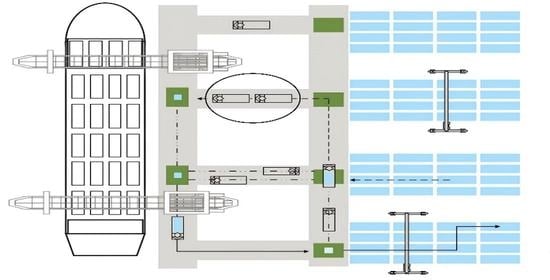
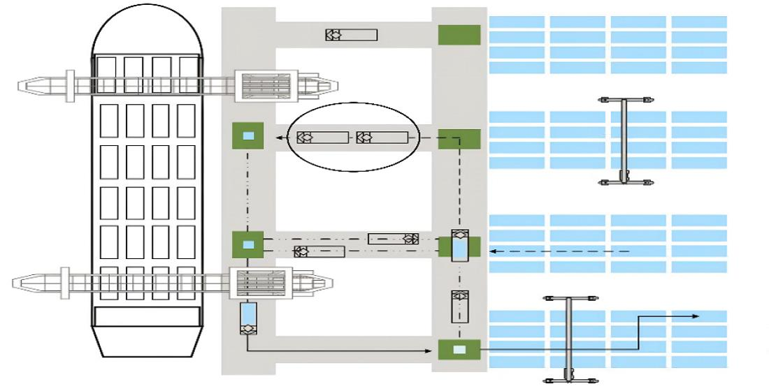
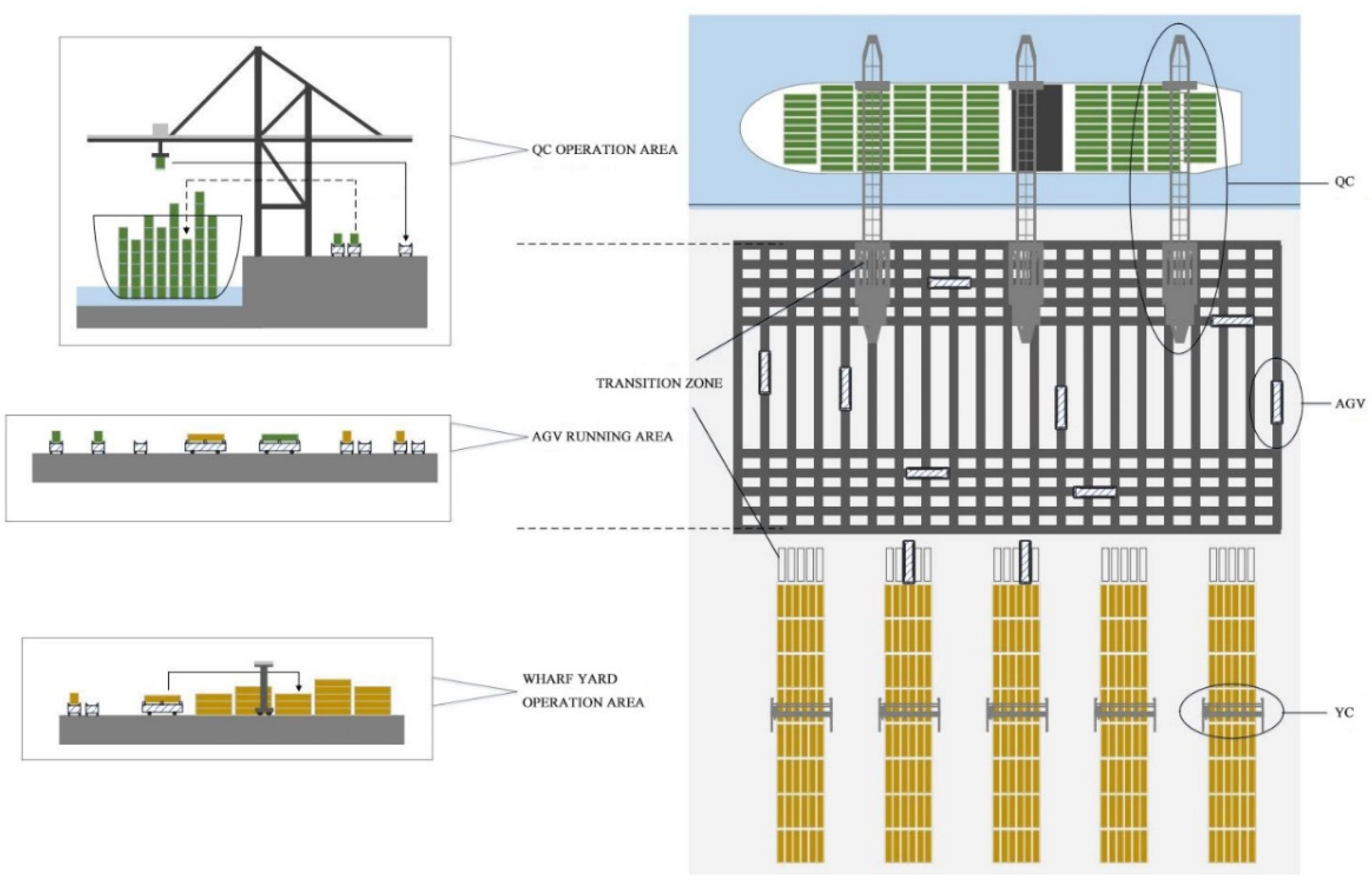
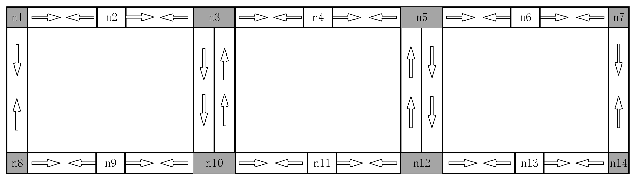
3.1. Problem Description

The layout of the automated container terminal is shown in Figure 1. The terminal operation relies on QCs, YCs and AGVs to realize container loading and unloading operation. Because the AGV does not have the function of loading and unloading containers, it needs to cooperate with the QCs and YCs to arrive at the designated handover place within the specified time to complete the horizontal transportation process between the wharf front and the yard. The single working efficiency of the two-trolley QCs in the automated wharf exceeds 30 working cycles per hour. However, according to the current equipment ratio in the wharf, the overall loading and unloading efficiency is only 25–29 container per hour, which has no obvious advantages compared with the traditional wharf. Increasing the size of AGV fleets performing horizontal transportation tasks can meet the requirements of efficient work in automated terminals, but with the expansion of fleet size, the occurrence frequency of congestion and deadlock problems on the running path of AGV will increase and the uncertainty of running time will be increased [22].

Different stacking positions of containers lead to different AGVs driving paths. Reasonable stacking positions of containers can reduce the running distance of AGV and improve the loading and unloading efficiency of the automated terminal is of great importance. However, it should not be ignored that the fleet size of AGV is too small to meet the efficiency requirements of other handling equipment in the automated terminal. Increasing the fleet size of AGVs performing horizontal transportation tasks can meet the requirements of efficient work in the automated terminal. However, large fleet size will lead to congestion and deadlock problems on the running path of AGVs, which will reduce the running speed of AGVs and increase the running time of AGVs [23].

As shown in Figure 2, the AGV scheduling scheme is further optimized by considering the congestion situation of the AGV on the running path and setting the congestion coefficient of the AGV in combination with the traffic flow theory, and the marks “n1, n2…n14” represented as hypothetical road nodes. By allocating the location of containers in the yard and determining the running path of AGV, it can be guaranteed to avoid AGV in the congested road section to a certain extent and reduce the no-load waste and running time of AGV on the road. By considering the uncertainty of AGV running time, the task assignment sequence of AGVs and the position of the inlet container in the yard were optimized to ensure the stability of the operating efficiency of the automated container terminal.

3.2. Model Construction

In order to better construct the model, the following assumptions are made in the research process:

(1)

The container handling sequence of QCs is known;

(2)

The export container sequence of YCs is known;

(3)

The number of containers, the number of AGVs, QCs and YCs are known;

(4)

AGVs, QCs and YCs can only handle one container at a time;

(5)

The impact of container turning and dumping in the yard on the production process of the automated YCs is not taken into account and there is enough free space in the yard to accommodate all the tasks that arrive at the ship;

(6)

Each AGV can serve multiple QCs and YCs;

(7)

When AGVs, QCs and YCs handle container loading and unloading tasks, they ignore the time when QCs or YCs release task container and lift task container.

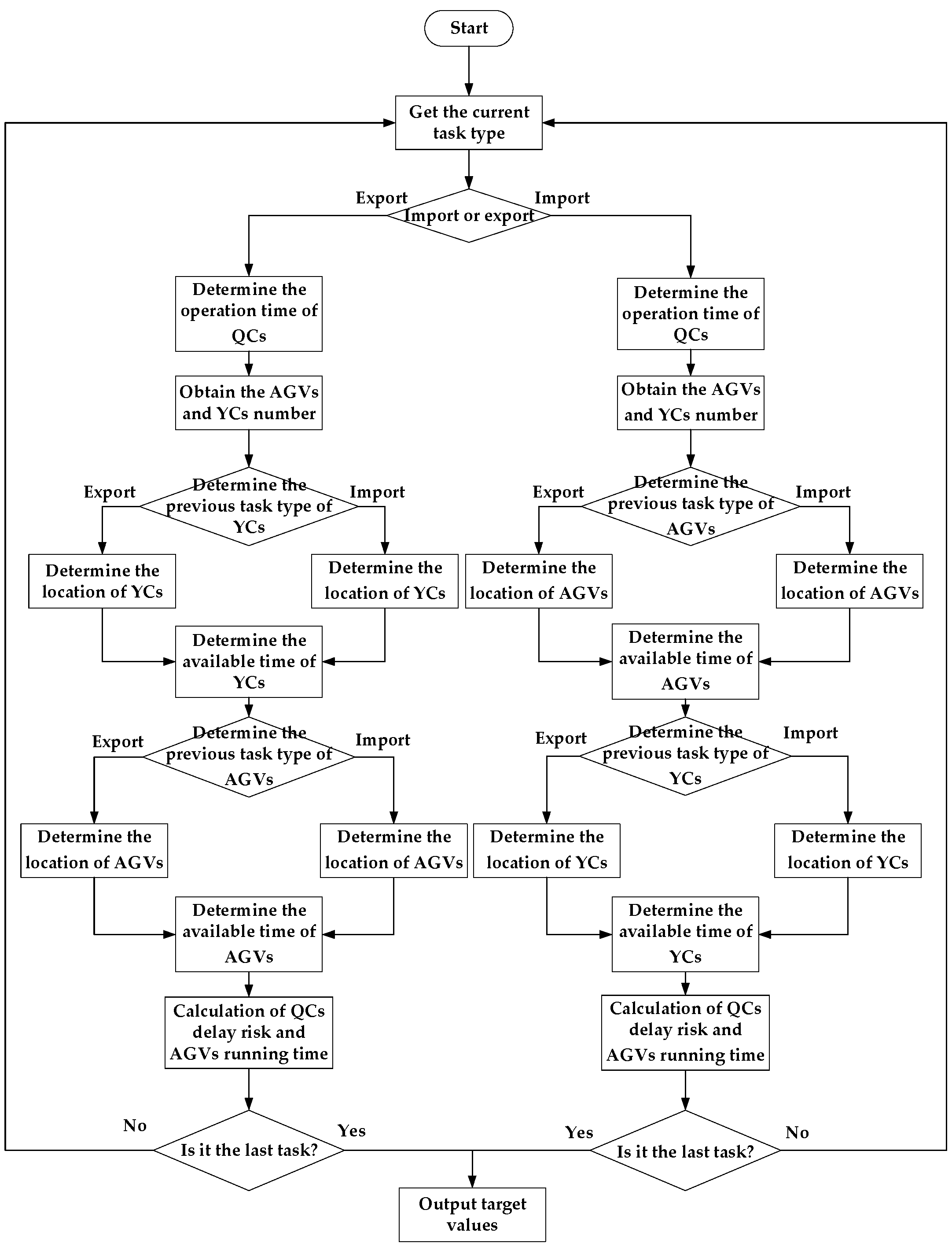
The operation process of QCs, YCs and AGVs is not disturbed by other external factors. Model parameters are set as follows:

V: collection of AGVs;

D: collection of imported containers;

L: collection of export containers;

N: collection of all containers;

P: refers to the position of the container in the yard;

Q: collection of QCs, k, r represents a single QC equipment;

Y: collection of YCs;

B: refers to the location of the container area in the yard. a, b represent the numbered location of the container area;

O_S: refers to the set of events including the virtual start event. (S, I) is the virtual start event;

O_F: refers to the set of events including virtual ending events. (F, I) is the virtual ending event;

O: collection of all tasks, among them $O=\{O_S,O_F\}\cup N$;

(i,k): the task i to be handled by QC k;

N_k: refers to the number of tasks (i,k) handled by QCs;

(n,b): refers to the task is located in b of the block n area in the yard;

h(i,k): refers to the operation time of QC k to process task (i,k), in seconds (s);

j(n,b): refers to the traveling time of YC between the transition zone of block n and position b, in seconds (s);

C_(i,k): the transition between AGV and QC (i = 1,2,3... m), if it is a loading operation, the QC picks up the container from the AGV; For ship unloading operation, the QC will place the container on the AGV;

U: collection of the event C_(i,k);

l(C_(i,k)): refers to the location of the event C_(i,k);

${\tilde{T}}_{irk}$: refers to the actual occurrence time of C_(i,k);

${\tilde{t}}_{ijk}$: refers to the travel time between the AGV at the transition zone n of QCs and the transition zone k of YCs; ${\tilde{t}}_{ijv}=\left(l_t,m_t,u_t\right)$ refers to the triangular fuzzy number representation of uncertain running time of AGV-v; where l_t refers to the optimal running time of ${\tilde{t}}_{ijk}$, $m_t$ refers to the most likely running time of ${\tilde{t}}_{ijk}$ and $u_t$ refers to the least ideal running time of ${\tilde{t}}_{ijk}$;

${\tilde{h}}_{i\mathrm{v}}=\left(l_h,m_h,u_h\right)$: refers to the time it takes AGV v to reach l(C_(i,k)), expressed by triangular fuzzy number;

$S_{ir}$: refers to the time when QC r arrives at position l(C_(i,k)) and is ready to operate C_(i,k);

$Y_{ikv}$: refers to the time when YC k arrives at the transition zone to pick up the container (i, k) from the AGV v or to place the container (i, k) on the AGV v;

Based on the traffic flow theory, this paper determines the congestion degree of AGVs on the driving path through the following formula. The relationship between the number of AGVs (V), speed (s) and traffic flow density (β) on the same path is:

$$V=s\beta$$

(1)

The expression between speed and traffic density is:

$$s\left(\beta \right)=\frac{s_f}{{\beta }_{\max }}\beta$$

(2)

Among them, s_f is the driving speed in free flow and β_max is the maximum traffic flow density on the path.

On the specific path l, there are:

$$t_{}=\frac{l}{s_{}}$$

(3)

According to the time $t_0=\frac{l}{s_f}$ required for the AGV to run in the free flow state, the running time of the AGV in specific path is:

$$t=t_0\left(\frac{2}{\left(1+\sqrt{1-\frac{4V}{s_f{\beta }_{\max }}}\right)}\right)$$

(4)

The optimal scheduling model established in this paper is as follows:

$$f_1=\min {\displaystyle \sum _{(i,k)\in O_S}{\displaystyle \sum _{(j,l)\in O_F}{\displaystyle \sum _{v\in V}{x}_{(i,k)}^{(j,l)}{\tilde{t}}_{ijv}}}}$$

(5)

$$f_2=\min {\displaystyle \sum _{i\in N}{\displaystyle \sum _{v\in V}{\xi }_{iv}}}$$

(6)

Equations (5) and (6) are objective functions, where (5) means the minimum running time cost of minimizing AGVs and (6) means the minimum delay risk of minimizing QCs.

$$s.t.{\displaystyle \sum _{(i,k)\in O_S}{x}_{(i,k)}^{(j,l)}}=1,\forall (j,l)\in N$$

(7)

$${\displaystyle \sum _{(j,l)\in O_F}{x}_{(i,k)}^{(j,l)}}=1,\forall (i,k)\in N$$

(8)

Equations (7) and (8) ensure that when the AGV executes task (i,k) or task (j,l), there is only one immediate front task (i,k) and immediate back task box (j,l) for each current task.

$${\displaystyle \sum _{(i,k)\in N}{x}_{(i,k)}^{(F,I)}}=v$$

(9)

$${\displaystyle \sum _{(j,l)\in N}{x}_{(S,I)}^{(j,l)}}=v$$

(10)

Equations (9) and (10) ensure that the total number of AGVs devices used in the model is the same as the number of configurations v in the automation dock.

$${\displaystyle \sum _{(i,k)\in D\cup (S,I)}{\sigma }_{(i,k)}^{(j,l)}}=1,\forall (j,l)\in D$$

(11)

$${\displaystyle \sum _{(i,k)\in D\cup (F,I)}{\sigma }_{(i,k)}^{(j,l)}}=1,\forall (j,l)\in L$$

(12)

$${\displaystyle \sum _{(i,k)\in L\cup (S,I)}{\sigma }_{(i,k)}^{(j,l)}}=1,\forall (j,l)\in D$$

(13)

$${\displaystyle \sum _{(i,k)\in L\cup (F,I)}{\sigma }_{(i,k)}^{(j,l)}}=1,\forall (j,l)\in L$$

(14)

Equations (11)–(14) are to ensure that there is only one immediate task (i,k) and one immediate task (j,l) when the automatic field bridge configured at each Block n in the yard processes the current task;

$${\displaystyle \sum _{(i,k)\in \mathrm{D}/L}{x}_{(i,k)}^{(F,I)}}=c$$

(15)

$${\displaystyle \sum _{(j,l)\in \mathrm{D}/L}{x}_{(S,I)}^{(j,l)}}=c$$

(16)

Equations (15) and (16) ensure that the total number of YCs used in the model is c;

$${\displaystyle \sum _{b\in B}{y}_{(i,k)}^b}=1,\forall (i,k)\in D$$

(17)

Equation (17) ensures that the bay b of the block in the yard leaves a vacant place for container storage;

$${\displaystyle \sum _{(n,b)\in D}{z}_{(i,k)}^{(n,b)}}=1,\forall (i,k)\in D$$

(18)

$${\displaystyle \sum _{(i,k)\in D}{z}_{(i,k)}^{(n,b)}}\le 1,\forall (n,b)\in P$$

(19)

$${\displaystyle \sum _{n\in N^{+}}{z}_{(i,k)}^{(n,b)}}=y_{(i,k)}^b,\forall (i,k)\in D,\forall b\in B$$

(20)

Equations (18)–(20) ensure that sufficient allocated positions (n,b) are left for import containers in the storage yard during loading and unloading, which conform to the allocation principle of container space in the container block of wharf.

$$q_{(i+1,k)}-q_{(i,k)}\ge h_{(i,k)},\forall (i+1,k)(i,k)\in 1,2,\cdot \cdot \cdot ,N-1$$

(21)

Equation (21) ensures the time relationship between the QCs and the task processing. It is that the starting time of the sequence task (j,l) after QC k processing should not be less than the sum of the time spent in processing the sequence task (i,k) before it.

$$d_{(i,k)}+2{\displaystyle \sum _{b\in P}{\varphi }_{(n,b)}{y}_{(i,k)}^b\le }{d}_{(j,l)}+M(1-{\sigma }_{(i,k)}^{(j,l)}),\forall (i,k)\in D,(j,l)\in D$$

(22)

$$d_{(i,k)}+2{\varphi }_{(n,b)}\le d_{(j,l)}+M(1-{\sigma }_{(i,k)}^{(j,l)}),\forall (i,k)\in L,(j,l)\in L$$

(23)

Equations (22) and (23) ensure the continuity of any YCs processing task. It is that the sum of the time spent to process the current assigned task (i,k) or the current assigned task (j,l) should be less than the starting time of the next assigned task (j,k) or the next assigned task (j,l);

$$q_{(i,k)}+h_{(i,k)}+t_{(i,k)}^{}\le d_{(i,k)},\forall (i,k)\in D$$

(24)

$$d_{(i,k)}+2{\phi }_{(n,b)}^{}+t_{(i,k)}\le q_{(j,l)},\forall (i,k)\in L$$

(25)

Equations (24) and (25) ensure the continuity of handling the export and import tasks in the entire automated terminal system. If it is the exit task, the sum of the starting time of YCs processing task (i,k), the time spent in YCs operation and the traveling time of the AGVs processing task (i,k) on the running path should be less than the starting time of the QCs processing task q_(i,k); similarly, for the import task, the sum of the starting time $q_{(i,k)}$ of QC k processing task (i,k), the time of QC k processing container and the traveling time of AGVs processing task (i,k) on the running path should be less than the starting time of YCs processing task (i,k).

$${\tilde{T}}_{jlv}-\left({\tilde{T}}_{ikv}+{\tilde{t}}_{ijv}\right)\ge M\left(1-x_{ijv}\right),\forall i\in O_S,\forall j\in O_F,\forall v\in V,\forall k,l\in Q$$

(26)

Equation (26) ensures that the time interval between the occurrence of two C_(i,k) events must be greater than the time required for AGVs operation; In the Equation (26), the value of ${\tilde{T}}_{jlv}$ is equal to the greater value of ${\tilde{h}}_{jv}$ and $S_{jl}$. Since the running time of AGVs is uncertain, the time of ${\tilde{T}}_{jlv}$ cannot be determined, so it is expressed by fuzzy number.

As shown in Figure 3, the value of ${\tilde{T}}_{jlv}$ in three different situations $S_{jl}<l_h$, $l_h\le S_{jl}\le u_h$ and $S_{jl}>u_h$ is shown in the shaded part. When $S_{jl}>u_h$, ${\tilde{T}}_{jlv}=S_{jl}$.

$$Y_{j{n}^{\prime }v}-\left(Y_{inv}+{\tilde{t}}_{ijv}\right)\ge M\left(1-x_{ijv}\right),\forall i\in D_o,\forall j\in D_f,\forall v\in V,\forall n,n^{\prime }\in Y$$

(27)

$${\tilde{T}}_{\left(i+1\right)rv}-{\tilde{T}}_{irv}\ge S_{\left(i+1\right)r}-S_{ir},\forall i\in O_S,\forall v\in V,\forall r\in Q$$

(28)

$${\tilde{T}}_{irk}={\tilde{S}}_{ir}\vee {\tilde{h}}_{ik},\forall i\in D,\forall k\in V,\forall r\in Q$$

(29)

$${\xi }_{iv}=\frac{area{\tilde{T}}_{irv}}{area{\tilde{h}}_{iv}},\forall i\in O,\forall v\in V,\forall r\in Q$$

(30)

Equation (27) ensures that the time interval for the YC to perform container loading and unloading operations must be greater than the time required for the AGVs operation; Equation (28) ensures that the time interval between the occurrence of two events C_(i,k) must be greater than the time required the QC operation. Equation (29) is to ensure that the occurrence time of C_(i,k) is the latest time when the QC and AGV arrive at position l(C_(i,k)). Equation (30) represents the delay risk of QCs; Where, ξ_ir represents the risk parameter leading to the QC delay after the AGV delay is reached, as shown in Figure 4 The value of ξ_ir is determined by ${\tilde{T}}_{irk}$ and ${\tilde{h}}_{ik}$, ${\xi }_{iv}=\frac{area{\tilde{T}}_{irk}}{area{\tilde{h}}_{ik}}$.

$$x_{(i,k)}^{(j,l)},y_{(i,k)}^b,z_{(i,k)}^{(n,b)},{\sigma }_{(i,k)}^{(j,l)}\in \{0,1\},\forall (i,k),(j,l)\in O,\forall b\in B$$

(31)

$$q_{(i,k)},p_{(i,k)},d_{(i,k)}\ge 0,\forall (i,k)\in N,i=1,2,\cdot \cdot \cdot ,N_k,\forall k\in K$$

(32)

Equations (31) and (32) define the variable types and value ranges of the above constraints in the model.

4. Solving Model

4.1. Model Transformation

For the scheduling optimization problem under uncertain environment, Sakawa, M. proposed two kinds of fuzzy operations according to the extended principle and related definitions of fuzzy mathematics [24]. Assuming that $\tilde{x}=\left(p,r,q\right)$ and $\tilde{y}=\left(l,m,u\right)$ are two triangular fuzzy numbers, the summation operation is $\tilde{x}+\tilde{y}=\left(p+l,r+m,q+u\right)$; When calculating the maximum value of two triangular fuzzy numbers, it is a simple operation and the result is approximately considered to be triangular fuzzy numbers, so: $\tilde{x}\vee \tilde{y}=\left(p,r,q\right)\vee \left(l,m,u\right)\approx \left(p\vee l,r\vee m,q\vee u\right)$.

According to the above fuzzy operation rules, the arrival time $S_{ir}$ of the QC in constraint (29) is expressed as triangular fuzzy number with three overlapping points, then constraint (29) can be expressed as:

$${\tilde{T}}_{irk}=S_{ir}\vee {\tilde{h}}_{ik}=\left(l_s,m_s,u_s\right)\vee \left(l_h,m_h,u_h\right)\approx \left(l_s\vee l_h,m_s\vee m_h,u_s\vee u_h\right),\forall i\in D,\forall k\in V,\forall r\in Q$$

(33)

The values $f_1^l$, $f_1^m$ and $f_1^u$ of the three endpoints of the fuzzy objective function $f_1=\min {\displaystyle \sum _{(i,k)\in O_S}{\displaystyle \sum _{(j,l)\in O_F}{\displaystyle \sum _{v\in V}{x}_{(i,k)}^{(j,l)}{\tilde{t}}_{ijv}}}}$ are obtained by l_t, m_t and u_t of the fuzzy running time ${\tilde{t}}_{ijv}$, respectively.

Step 1: Transform the original fuzzy objective function (5) into a multi-objective linear programming function:

$$\{\begin{array}{l}\max {\lambda }_1=f_1^m-f_1^l\\ \max {\lambda }_2=f_1^m\\ \min {\lambda }_3=f_1^u-f_1^m\end{array}$$

(34)

wherein, take the extremum of ${\lambda }_1$, ${\lambda }_2$ and ${\lambda }_3$, and its purpose is to minimize the AGV’s total elapsed time in the most likely, ideal and least ideal cases.

Step 2: According to the Zimmermann method [25], the positive and negative ideal values of ${\lambda }_i\left(i=1,2,3\right)$, ${\lambda }_i^{PIS}$ and ${\lambda }_i^{ZIS}$, can be obtained, respectively and the membership function ${\mu }_i\left(i=1,2,3\right)$ can be determined to indicate the satisfaction degree of ${\lambda }_i$.

$${\lambda }_1^{PIS}=\max \left\{f_1^m-f_1^l\right\};{\lambda }_2^{PIS}=\min f_1^m;{\lambda }_3^{PIS}=\min \left\{f_1^u-f_1^m\right\};$$

$${\lambda }_1^{NIS}=\min \left\{f_1^m-f_1^l\right\};{\lambda }_2^{NIS}=\max f_1^m;{\lambda }_3^{NIS}=\max \left\{f_1^u-f_1^m\right\}\text{.}$$

${\lambda }_i$(i = 1,2,3) membership function is:

$$u_i=\{\begin{array}{l}0,x>{\lambda }_i^{NIS}\\ \frac{x-{\lambda }_i^{NIS}}{{\lambda }_i^{PIS}-{\lambda }_i^{NIS}},{\lambda }_i^{PIS}\le x\le {\lambda }_i^{NIS}\\ 1,x<{\lambda }_i^{PIS}\end{array}$$

(35)

$$f_1^{\prime }=\max \left\{\epsilon {\delta }^u+\left(1-\epsilon \right){\delta }^l\right\}$$

(36)

$$s.t.{\delta }^l\le {\mu }_i\le {\delta }^u,i=1,3$$

(37)

$${\mu }_2\ge {\delta }^u$$

(38)

$${\delta }^l,{\delta }^u\in \left[0,1\right]$$

(39)

where ${\delta }^u$ represents the maximum value of membership function and ${\delta }^l$ represents the minimum value of membership function, where m_i(i = 1, 2, 3) and the complement operator ε represents the degree of tendency of decision-makers in positive or negative decisions. The greater the value of ε, the greater the proportion of ${\delta }^u$ in the objective function (36) and the more positive the decisions are made; otherwise, the more negative decisions are made. In this paper, under the condition of comprehensive consideration of the best and worst cases, the running time of AGV is minimized and ${\mu }_2$ is made to obtain the maximum membership function and then solved by combining with the improved genetic algorithm.

For the objective function (6), the connection process between AGV and QC in the working process is taken as an example and the task information is shown in

Table 1. Task information.

QC
Task Order	Type	Position in Ship	Position in Yard	QC (s)	AGV-1 (s)	AGV-2 (s)
i	shipment	12/03/04	C/21/4/4	200	(150,200,210)	(180,200,220)

.

When task i is performed by AGV-1, ${\tilde{T}}_{ir1}=\left(200,200,210\right)$, ${\xi }_{\mathrm{i}}=0.167$ can be obtained according to constraint (29) and (30). When task i is performed by AGV-2, ${\tilde{T}}_{ir2}=\left(200,200,220\right)$, ${\xi }_{\mathrm{i}}=0.5$ are performed by AGV-1 because the risk of arriving at the exchange site late is lower when task i is performed by AGV-1.

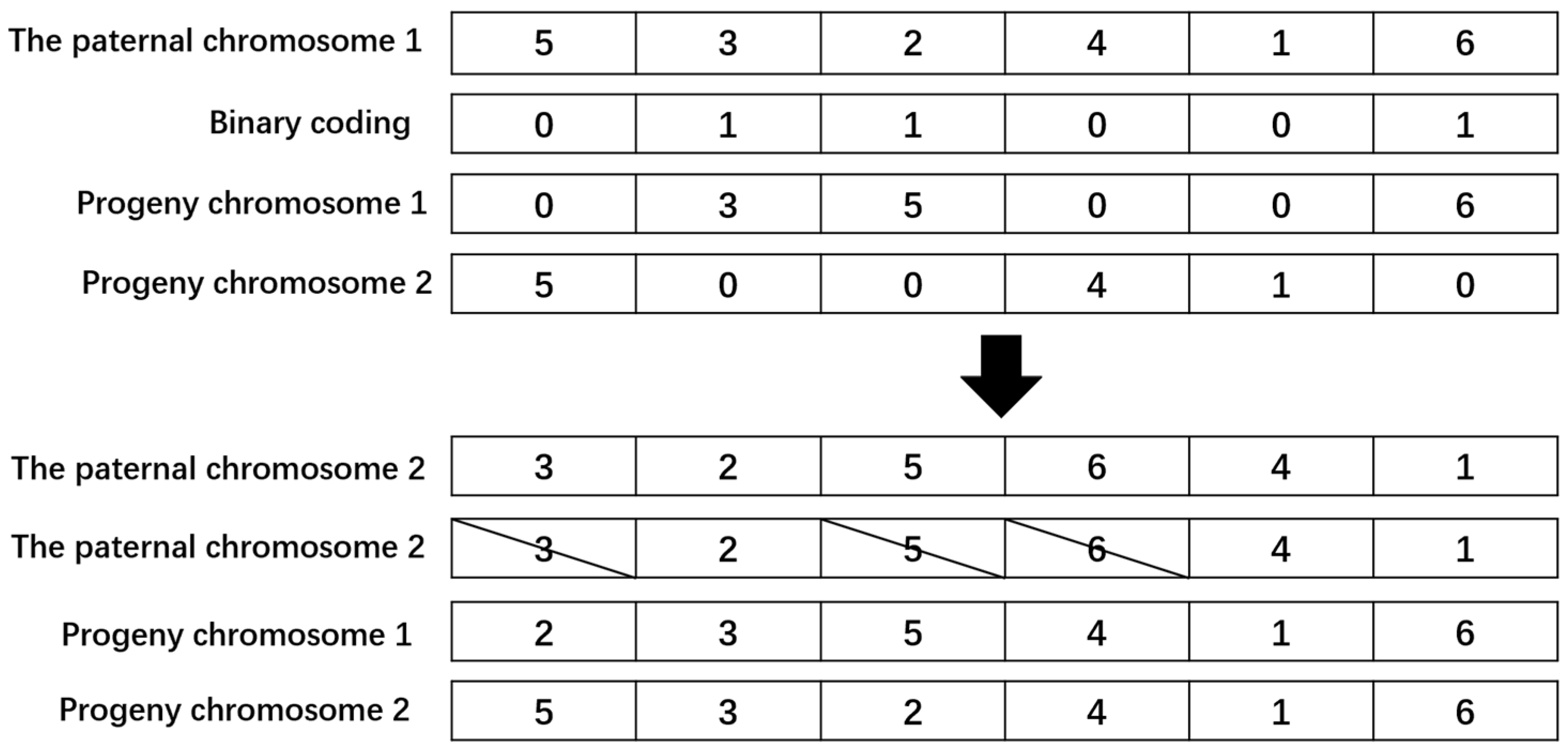
4.2. Algorithm Design

The AGV scheduling optimization problem studied in this paper has been proved to be NP-hard problem [26]. Due to the large scale of the problem in practical application, it is difficult to obtain the accurate optimal solution within the effective time. The AGV running time in this paper is uncertain and the fuzzy mathematics method is adopted to deal with the uncertainty of data, which increases the complexity of the model. It cannot be solved by traditional analytical methods. This paper presents an improved genetic algorithm, which solves the scheduling problem effectively and improves the performance of the traditional genetic algorithm.

• Construct chromosomes and generate initial population

In this paper, the initial task is n randomly generated sequences. As for the relationship between container serial number and import or export, import containers are represented by even numbers, while export containers are represented by odd numbers. The chromosome coding representation is shown in Figure 5. The AGV number assigned to each task randomly generated by the first chromosome behavior; the second chromosomal behavior randomly assigned the location of each import container yard, in which, after the initial allocation of the container position, the export container will not change after the completion of the allocation and the import container will change in the subsequent genetic operations. The initial feasible solution was detected, the infeasible solution was deleted, the feasible solution was retained and the chromosome sequence was regenerated at the position of the infeasible solution and the cycle operation was carried out until all the solutions were feasible to ensure the feasibility of the initial population [27].

• Calculation of objective function

In the process of calculating the objective function value, the congestion situation on the path is set according to Equations (1)–(4) and the running time of the AGV when performing the task is depicted as a triangular fuzzy number according to the congestion coefficient. The specific calculation process is shown in Figure 6.

• Fitness calculation

By summation of the running time of AGV in the above calculated objective function, the value $f_1^l$, $f_1^m$, $f_1^u$ of objective function $f_1=\min {\displaystyle \sum _{(i,k)\in O_S}{\displaystyle \sum _{(j,l)\in O_F}{\displaystyle \sum _{v\in V}{x}_{(i,k)}^{(j,l)}{\tilde{t}}_{ijv}}}}$ can be obtained. and $f_1{}^{\prime }$ can be obtained through transformation. According to the above objective function $f_2=\min {\displaystyle \sum _{i\in N}{\displaystyle \sum _{v\in V}{\xi }_{iv}}}$, the sum of the delay risk $f_2$ of the automated QCs is obtained. According to Equations (7)~(37), the value of multiple objective function is obtained. The objective function of the nth chromosome is: $Z_n=\alpha \raisebox{1ex}{${f^{\prime }}_{1n}$}\!\left/ \!\raisebox{-1ex}{${\overline{f^{\prime }}}^{}{}_{1n}$}\right.+\frac{1}{m}\left(1-\alpha \right)f_{2n}$. Where, ${\overline{f^{\prime }}}^{}{}_{1n}$ represents the mean value of the objective function and the fitness of the chromosome is ${\theta }_n=\frac{1}{Z_n}$. The greater the value of ${\theta }_n$, the closer the obtained result is to the optimal solution.

• Genetic manipulation

Selection: for each generation of the population, the roulette method is used for gene selection and the chromosome with the greatest fitness value is directly copied into the next generation of the population. The probability of individual selection is $P_i={\theta }_i/{\displaystyle \sum _{k=1}^{P_s}{\theta }_n}$, where population size is $P_s$ and fitness of individual i is ${\theta }_n$.

Crossover: Single-point crossover operator is used to perform crossover operation on the first line of the chromosome. Since AGV in the model can operate on both import and export containers, uniform sorting crossover operator is used to perform crossover operation on the second line of the chromosome in order to maintain the feasibility of individuals in the chromosome.

As shown in Figure 7, the parent chromosomes 1 and 2 are represented by six import containers and their storage positions in the storage yard have been generated. Uniform sort crossover operator is used in this paper. First, a number sequence composed of 0 and 1 is generated corresponding to chromosomes. If the individual in the parent chromosome 1 corresponds to the number sequence “1”, it will be passed on to the child chromosome 1. If the individual on the parent chromosome 1 corresponds to “0”, it is passed on to the child chromosome 2. Paternal chromosome 2 is the opposite. New progeny chromosomes were generated after uniform sequencing and crossover. In the process of mutation, the basic location mutation operator is used to designate each locus of two chromosomes of each individual as the mutation point according to the mutation probability and the gene value of the mutation point is regenerated.

Convergence judgment: judge whether the difference between the average fitness value and the minimum fitness value in the population is less than the predetermined threshold value, or whether the evolutionary algebra reaches the preset maximum iteration number. If true, the calculation ends and the optimal scheduling scheme is obtained; otherwise, it is executed.

5. Analysis of Calculation Examples

5.1. Basic Parameter Setting

In order to verify the effectiveness of the algorithm and model in this paper and solve the task assignment problem of AGVs, this paper takes the layout of the automated container terminal of Shanghai as the background and sets the basic data used in the calculation process on this basis.

The parameter Settings used in this article are as follows:

(1)

The number of containers set in many examples in this experiment varies from 1 to 500, of which 4–30 containers are used for small-scale example problems and 30–500 containers for large-scale example problems. In addition, the number of quay and tank areas in the range of 2–8 was considered and the number of AGVs ranged from 4 to 24.

(2)

In this experimental example, the data are set according to the actual port operation value. Among them, the horizontal speed of the AGV is 5 m/s, the length of the AGV operation area is 240 m, the width of the AGV operation area is 100 m and the distance between adjacent auxiliary roads is 30 m.

(3)

Based on the preliminary experiment, genetic parameters were set, including the crossover rate (Pc) of 0.8, mutation rate (Pm) of 0.01, population size (Ps) of 50 and the maximum iteration algebra (Mg) of 500 [28].

5.2. Feasibility Analysis of Algorithm

In this paper, the task assignment of AGV considering uncertainty and the optimization of the storage location of the storage yard are NP-hard problems. With the expansion of the size of the calculating examples, the number of feasible solutions of the problem increases geometrically and CPLEX can only solve the small-scale calculating cases within the effective time. According to the above model and algorithm, we program in MATLAB software. In this chapter, heuristic algorithm is used to calculate the large-scale calculating cases. CPLEX was used to verify the effectiveness of the heuristic algorithm. Taking 24 AGVs as an example, according to the path shown in Figure 2, the running time of AGVs is shown in the following table.

To verify the effectiveness of the heuristic algorithm, 12 small experiments were conducted, with the number of containers ranging from 4 to 30.

Table 2. AGV running time.

	n1	n3	n5	n7	n8	n10	n12	n14
n1	(0, 0, 0)	(20, 21, 22.2)	—	—	(30, 31.5, 33.3)	—	—	—
n3	(20, 21, 22.2)	(0, 0, 0)	(20, 21, 22.2)	—	—	(30, 35.4, 39)	—	—
n5	—	(20, 21, 22.2)	(0, 0, 0)	(20, 21, 22.2)	—	—	(30, 35.4, 39)	—
n7	—	—	(20, 21, 22.2)	(0, 0, 0)	—	—	—	(30, 31.5, 33.3)
n8	(30, 31.5, 33.3)	—	—	—	(0, 0, 0)	(20, 21, 22.2)	—	—
n10	—	(30, 35.4, 39)	—	—	(20, 21, 22.2)	(0, 0, 0)	(20, 21, 22.2)	—
n12	—	—	(30, 35.4, 39)	—	—	(20, 21, 22.2)	(0, 0, 0)	(20, 21, 22.2)
n14	—	—	—	(30, 31.5, 33.3)	—	—	(20, 21, 22.2)	(0, 0, 0)

shows the comparison between the results of CPLEX and the heuristic algorithm in the small calculation cases. The improved genetic algorithm has more advantages than CPLEX in the calculation speed. The calculation time of CPLEX is in the range of 23.2 s to 12734.7 s and it cannot solve the large-scale calculation cases with more than 24 task boxes in the effective time. However, the operation time of the improved genetic algorithm proposed in this paper is from 2.7 s to 4.5 s and the average difference rate (GAP) of the objective function value is 5.4%, which means that the algorithm proposed in this paper can get a satisfactory solution in a short time. By analyzing the comparison of experimental data in

Table 3. Comparison results of small-scale examples.

No.	Number of Tasks	QCs-AGVs-YCs	CPLEX(MILP)		Heuristic Algorithm			GAP (%)
			Computation Time (s)	Completion Time (s)	Computation Time (s)	Completion Time (s)	Function Value
1	4	2-4-3	23.2	153	3.4	161	3.07	5.2
2	6	2-4-3	69.6	199	2.7	208	3.94	4.5
3	8	2-4-3	214.5	243	2.9	258	3.36	6.2
4	10	3-4-5	935.5	246	2.9	260	2.35	5.7
5	10	3-12-5	1037.1	176	3.8	185	4.25	5.1
6	12	3-12-5	2718.9	213	3.9	224	3.44	5.2
7	12	3-15-5	2986.1	147	3.4	159	4.57	8.2
8	16	3-15-5	6803.2	198	3.0	210	3.96	6.1
9	16	4-8-6	5917.2	270	3.2	280	5.64	3.7
10	24	4-16-6	12,734.7	243	3.5	253	4.47	4.1
11	30	5-10-8	>14,400	—	4.1	325	5.47	—
12	30	5-15-8	>14,400	—	4.5	302	6.17	—

Note: GAP = (|completed time of heuristic algorithm—completed time of CPLEX)/completed time of CPLEX × 100%.

, it can be seen that the growth trend of completion time of dock loading and unloading is consistent with that of the number of containers (Example 5 and 6 and Example 7 and 8). According to Example 4 and 5 and Example 7 and 8, it can be seen that the loading and unloading completion time can be reduced by increasing the number of AGVs.

As can be seen from the experimental results in

Table 4. Large-scale examples.

No.	Number of Tasks	QCs-AGVs-YCs	Heuristic Algorithm
			Computation Time (s)	Completion Time (s)	Function Value
13	35	2-4-3	3.45	898	8.74
14	35	2-8-3	4.30	518	11.38
15	35	2-16-3	8.90	416	14.98
16	65	2-8-3	9.03	969	8.61
17	120	2-8-3	28.52	1739	5.36
18	35	3-6-5	11.73	573	7.80
19	35	3-12-5	11.27	293	12.08
20	35	3-15-5	12.84	225	14.56
21	65	3-12-5	23.13	651	7.95
22	120	3-12-5	19.33	1254	6.37
23	65	4-8-6	4.01	947	8.91
24	65	4-12-6	5.81	563	8.82
25	65	4-16-6	13.43	487	11.27
26	240	4-16-6	55.91	1864	10.33
27	120	5-10-8	9.51	1443	8.33
28	120	5-20-8	11.99	815	15.71
29	240	5-20-8	44.20	1527	14.25
30	240	6-12-10	27.50	2344	8.12
31	240	6-24-10	37.67	1282	12.96
32	320	6-24-10	96.76	1641	10.77
33	320	8-16-10	35.07	2376	10.92
34	320	8-24-10	49.30	1285	16.73
35	500	8-16-10	53.07	2924	5.22
36	500	8-24-10	114.65	2678	16.11

, a better fitness function value can be obtained within a reasonable calculation time by using the improved genetic algorithm to solve large-scale examples. In the 36th example, the number of containers is 500 and the calculation time is 114 s, indicating that the improved genetic algorithm can significantly reduce the calculation time. Under the same conditions, increasing the number of containers will also increase the completion time of loading and unloading operations, as shown in examples 16 and 17 and 21 and 22. When the number of containers remains the same, the increase in the number of AGVs leads to a smaller completion time, that is, faster loading and unloading at the terminal, as shown in examples 14 and 15 and 19 and 20. The experimental results of Example 14 and 15 and 17–20 show that when the number of containers remains the same, the fitness function value increases by adjusting the proportion to the quantity of QC. The reason is that when the proportion of AGVs to QCs increases, the QC waiting time decreases, the objective function value decreases and the fitness function value increases. (The data and AGVs scheduling scheme for example 36 are shown in Supplementary Materials.)

According to the above experiments, if the ratio of AGVs to QCs and YCs is increased within a certain range, the completion time will be reduced correspondingly, that is, the loading and unloading efficiency will be improved in terminal. However, when the number of AGVs increased by 4 times as much as that of QCs, the difference in the completion time between the number of AGVs increased by 5 times as much as that of the QCs was small. Therefore, we took the cost factor into consideration in the actual operation and the use of 4 times as many AGVs could meet the requirements of the automated terminal operation.

In order to verify the advantages of applying fuzzy mathematics theory to solve AGVs scheduling and optimization problems with uncertain running time, a comparison model is proposed. The uncertainty of the AGV running time is not considered in the comparison model and the AGVs running time is represented by the most likely time mt in the triangular fuzzy number ${\tilde{t}}_{ijv}=\left(l_t,m_t,u_t\right)$. The other parts are the same as the optimization model considering the uncertain running time. The comparative experimental results are analyzed from the following two aspects.

(1)

The maximum completion time of the quay under the two methods was compared with the time when the QC finished processing the last task as the standard.

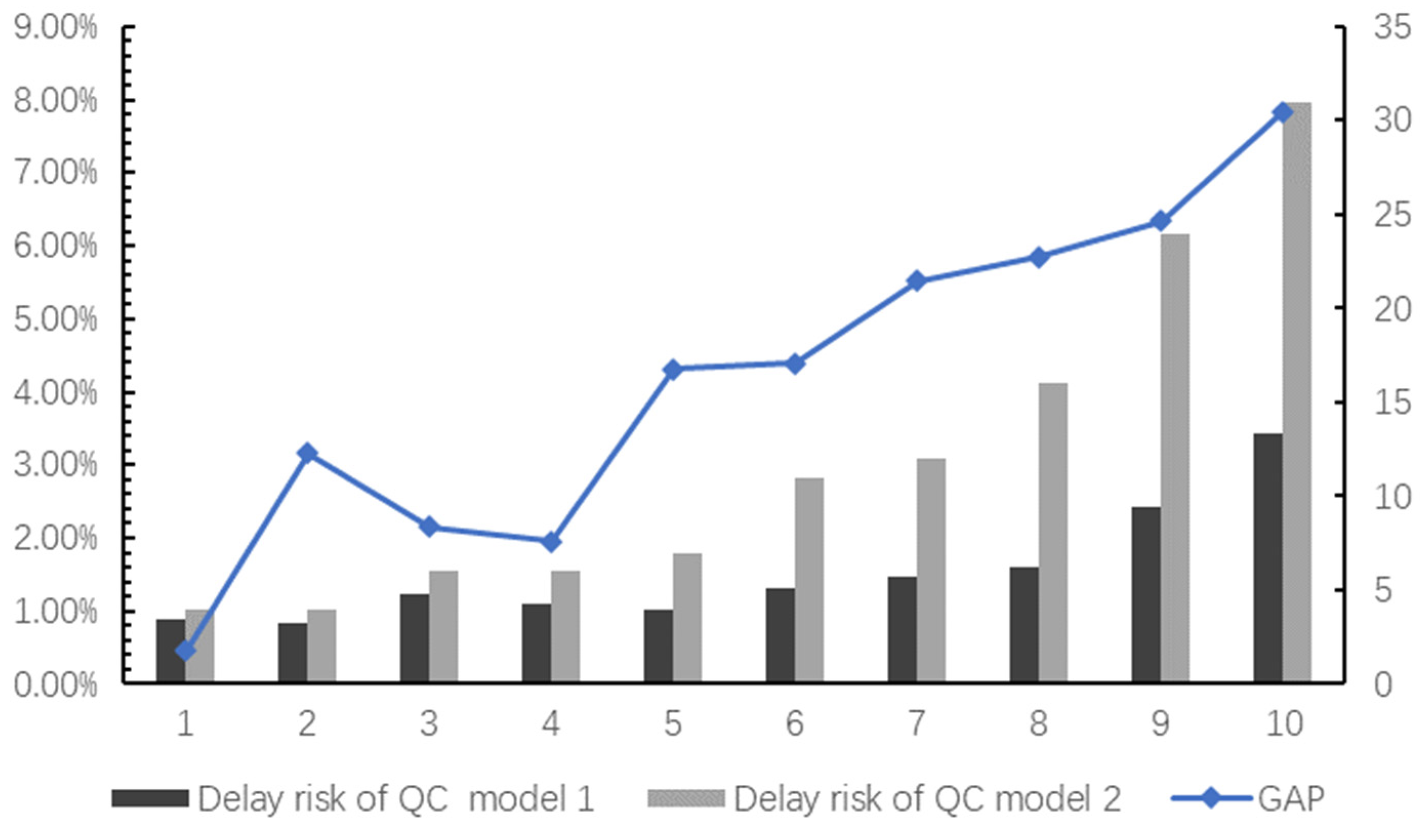
(2)

Compare the sum of delay risks of QCs processing tasks.

In the comparison model, the decision variable birv is set to represent the QCs delay risk. If the time for AGV to reach the quay front transition zone is later than the time for the corresponding QC to prepare for the task, i.e., h(i,k) > Sir, the QCs delay risk b_irv= 1; b_irv = 0 otherwise.

$$E={\displaystyle \sum _{i\in O}{\beta }_{ir\mathrm{v}}},\forall v\in V,\forall r\in Q$$

(40)

The comparison model is as follows:

$$Min{\max }_k(q_{(N_k,k)}+h_{(N_k,k)})$$

(41)

$$s.t.{\displaystyle \sum _{(i,k)\in O_S}{x}_{(i,k)}^{(j,l)}}=1,\forall (j,l)\in N$$

(42)

$${\displaystyle \sum _{(j,l)\in O_F}{x}_{(i,k)}^{(j,l)}}=1,\forall (i,k)\in N$$

(43)

$${\displaystyle \sum _{(j,l)\in N}{x}_{(S,I)}^{(j,l)}}=v$$

(44)

$${\displaystyle \sum _{(i,k)\in N}{x}_{(i,k)}^{(F,I)}}=v$$

(45)

$${\displaystyle \sum _{(i,k)\in D\cup (S,I)}{\sigma }_{(i,k)}^{(j,l)}}=1,\forall (j,l)\in D$$

(46)

$${\displaystyle \sum _{(i,k)\in D\cup (F,I)}{\sigma }_{(i,k)}^{(j,l)}}=1,\forall (j,l)\in L$$

(47)

$${\displaystyle \sum _{(i,k)\in L\cup (S,I)}{\sigma }_{(i,k)}^{(j,l)}}=1,\forall (j,l)\in D$$

(48)

$${\displaystyle \sum _{(i,k)\in L\cup (F,I)}{\sigma }_{(i,k)}^{(j,l)}}=1,\forall (j,l)\in L$$

(49)

$${\displaystyle \sum _{(i,k)\in \mathrm{D}/L}{x}_{(i,k)}^{(F,I)}}=c$$

(50)

$${\displaystyle \sum _{(j,l)\in \mathrm{D}/L}{x}_{(S,I)}^{(j,l)}}=c$$

(51)

$${\displaystyle \sum _{b\in B}{y}_{(i,k)}^b}=1,\forall (i,k)\in D$$

(52)

$${\displaystyle \sum _{(n,b)\in D}{z}_{(i,k)}^{(n,b)}}=1,\forall (i,k)\in D$$

(53)

$${\displaystyle \sum _{(i,k)\in D}{z}_{(i,k)}^{(n,b)}}\le 1,\forall (n,b)\in P$$

(54)

$${\displaystyle \sum _{n\in N^{+}}{z}_{(i,k)}^{(n,b)}}=y_{(i,k)}^b,\forall (i,k)\in D,\forall b\in B$$

(55)

$$q_{(i+1,k)}-q_{(i,k)}\ge h_{(i,k)},\forall (i+1,k)(i,k)\in 1,2,\cdot \cdot \cdot ,N-1$$

(56)

$$d_{(i,k)}+2{\displaystyle \sum _{b\in P}{\varphi }_{(n,b)}{y}_{(i,k)}^b\le }{d}_{(j,l)}+M(1-{\sigma }_{(i,k)}^{(j,l)}),\forall (i,k)\in D,(j,l)\in D$$

(57)

$$d_{(i,k)}+2{\varphi }_{(n,b)}\le d_{(j,l)}+M(1-{\sigma }_{(i,k)}^{(j,l)}),\forall (i,k)\in L,(j,l)\in L$$

(58)

$$q_{(i,k)}+h_{(i,k)}+t_{(i,k)}^{}\le d_{(i,k)},\forall (i,k)\in D$$

(59)

$$d_{(i,k)}+2{\phi }_{(n,b)}^{}+t_{(i,k)}\le q_{(j,l)},\forall (i,k)\in L$$

(60)

$$T_{jlv}-\left(T_{ikv}+t_{ijv}\right)\ge M\left(1-x_{ijv}\right),\forall i\in O_S,\forall j\in O_F,\forall v\in V,\forall k,l\in Q$$

(61)

$$Y_{j{n}^{\prime }v}-\left(Y_{inv}+t_{ijv}\right)\ge M\left(1-x_{ijv}\right),\forall i\in D_o,\forall j\in D_f,\forall v\in V,\forall n,n^{\prime }\in Y$$

(62)

$$T_{\left(i+1\right)rv}-T_{irv}\ge S_{\left(i+1\right)r}-S_{ir},\forall i\in O_S,\forall v\in V,\forall r\in Q$$

(63)

$$T_{irk}=S_{ir}\vee h_{ik},\forall i\in D,\forall k\in V,\forall r\in Q$$

(64)

$$x_{(i,k)}^{(j,l)},y_{(i,k)}^b,z_{(i,k)}^{(n,b)},{\sigma }_{(i,k)}^{(j,l)}\in \{0,1\},\forall (i,k),(j,l)\in O,\forall b\in B$$

(65)

$${\beta }_{ir\mathrm{v}}\in \left\{0,1\right\},\forall v\in V,\forall r\in Q$$

(66)

$$q_{(i,k)},p_{(i,k)},d_{(i,k)}\ge 0,\forall (i,k)\in N,i=1,2,\cdot \cdot \cdot ,N_k,\forall k\in K$$

(67)

In the comparative experiment, the number of containers is controlled as 12, 24, 30, 65, 120, 240, 320, 500 and the proportion of loading and unloading equipment in the terminal is AGVs: QCs: YCs = 2:1:1. Basic data of (6), (10), (11), (16), (17), (22), (28), (31), (32) and (36) in the experimental group above are taken for comparative experiment and the experimental results are shown in

Table 5. Comparison of solution results.

No.	Completion Time (s)			Delay Risk of QCs
	Model 1	Model 2	GAP (%)	Model 1	Model 2
1	224	225	0.45%	3.5	4
2	253	261	3.16%	3.2	4
3	325	332	2.15%	4.8	6
4	969	988	1.96%	4.3	6
5	1739	1814	4.31%	4.0	7
6	1254	1309	4.39%	5.1	11
7	815	860	5.52%	5.7	12
8	1282	1357	5.85%	6.2	16
9	1641	1745	6.34%	9.4	24
10	2678	2888	7.84%	13.3	31

Note: An optimization model of integrated AGVs scheduling and container storage problems for automated container terminal considering uncertainty is defined as Model 1; Comparison Model is defined as Model 2. GAP = (|comparison model—AGV runtime uncertain scheduling model)/AGV runtime uncertain scheduling model × 100%.

:

Each of the above examples are calculated for 10 times, average, compared to consider running time uncertainty of AGVs scheduling optimization model and comparing the results of solving the model solution, compared with the model results, considering the running time of uncertain AGVs scheduling optimization plan can reduce the risk of land bridge delay, shortening makespan. The results are shown in Figure 8.

6. Conclusions

In this paper, a symmetric triangular fuzzy number is used to describe the uncertainty of AGV running time and the most satisfactory time, most possible time and most negative time of AGV running are determined according to different congestion coefficients. On this basis, a multi-objective scheduling optimization model based on the minimum delay risk and the shortest running time of AGV was established. A heuristic algorithm for solving the model is designed and compared with the results of CPLEX. The results show that the algorithm designed in this paper can quickly obtain the AGVs scheduling and container stacking schedule under uncertain running time. In order to verify the effectiveness of this model, it is compared with the traditional optimization model. The results show that this scheduling model can get the optimal scheduling scheme quickly and efficiently. Compared with the traditional optimization model, the scheduling scheme can effectively reduce the delay risk of QCs and improve the loading and unloading efficiency of terminal with the expansion of task scale.

This paper studies AGVs scheduling and container storage problems considering uncertainty. The scheduling of QCs and YCs is not considered. The further work is to study cooperative scheduling optimization among multiple devices considering uncertainty.

References

1. Bae, H.Y.; Choe, R.; Park, T.; Ryu, K.R. Comparison of operations of AGVs and ALVs in an automated container terminal. J. Intell. Manuf. 2011, 22, 413–426. [Google Scholar] [CrossRef]
2. Angeloudis, P.; Bell, M. An uncertainty-aware AGV assignment algorithm for automated container terminals. Transp. Res. Part E Logist. Transp. Rev. 2010, 46, 354–366. [Google Scholar] [CrossRef]
3. Gan, Y.; Ji, S.; Zhao, Q.; Guo, D. Scheduling problems of automated guided vehicles in automated container terminals using a genetic algorithm. In Proceedings of the IOP Conference Series: Materials Science and Engineering, Guangzhou, China, 27–29 December 2019; IOP Publishing: Bristol, UK, 2020; p. 012069. [Google Scholar]
4. Zheng, Y.; Xiao, Y.; Seo, Y. A tabu search algorithm for simultaneous machine/AGV scheduling problem. Int. J. Prod. Res. 2014, 52, 5748–5763. [Google Scholar] [CrossRef]
5. Rashidi, H.; Tsang, E. A complete and an incomplete algorithm for automated guided vehicle scheduling in container terminals. Comput. Math. Appl. Int. J. 2011, 61, 630–641. [Google Scholar] [CrossRef]
6. Fazlollahtabar, H.; Hassanli, S. Hybrid cost and time path planning for multiple autonomous guided vehicles. Appl. Intell. 2018, 48, 482–498. [Google Scholar] [CrossRef]
7. Ma, N.; Zhou, C.; Stephen, A. Simulation model and performance evaluation of battery-powered AGV systems in automated container terminals. Simul. Model. Pract. Theory 2020, 106, 102146. [Google Scholar] [CrossRef]
8. Xin, J.; Negenborn, R.R.; Lodewijks, G. Trajectory planning for AGVs in automated container terminals using avoidance constraints: A case study—ScienceDirect. IFAC Proc. Vol. 2014, 47, 9828–9833. [Google Scholar] [CrossRef] [Green Version]
9. Liu, C.I.; Jula, H.; Vukadinovic, K.; Ioannou, P. Automated guided vehicle system for two container yard layouts—ScienceDirect. Transp. Res. Part C Emerg. Technol. 2004, 12, 349–368. [Google Scholar] [CrossRef]
10. Zaghdoud, R.; Mesghouni, K.; Dutilleul, S.C.; Zidi, K.; Ghedira, K. A hybrid method for assigning containers to AGVs in container terminal. IFAC-Pap. 2016, 49, 96–103. [Google Scholar] [CrossRef]
11. Miyamoto, T.; Inoue, K. Local and random searches for dispatch and conflict-free routing problem of capacitated AGV systems. Comput. Ind. Eng. 2016, 91, 1–9. [Google Scholar] [CrossRef]
12. Li, Q.; Pogromsky, A.; Adriaansen, T.; Udding, J.T. A control of collision and deadlock avoidance for automated guided vehicles with a fault-tolerance capability. Int. J. Adv. Robot. Syst. 2016, 13, 64. [Google Scholar] [CrossRef] [Green Version]
13. Zhuang, Y.; Sharma, S.; Subudhi, B.; Huang, H.; Wan, J. Efficient collision-free path planning for autonomous underwater vehicles in dynamic environments with a hybrid optimization algorithm. Ocean Eng. 2016, 127, 190–199. [Google Scholar] [CrossRef] [Green Version]
14. Fan, X.; He, Q.; Zhang, Y. Zone design of tandem loop AGVs path with hybrid algorithm. IFAC-Pap. 2015, 48, 869–874. [Google Scholar] [CrossRef]
15. Lombard, A.; Perronnet, F.; Abbas-Turki, A.; El Moudni, A. Decentralized management of intersections of automated guided vehicles. IFAC-Pap. 2016, 49, 497–502. [Google Scholar] [CrossRef]
16. Luo, J.; Wu, Y.; Mendes, A.B. Modelling of integrated vehicle scheduling and container storage problems in unloading process at an automated container terminal. Comput. Ind. Eng. 2016, 94, 32–44. [Google Scholar] [CrossRef]
17. Chen, X.; He, S.; Zhang, Y.; Tong, L.C.; Shang, P.; Zhou, X. Yard crane and AGV scheduling in automated container terminal: A multi-robot task allocation framework. Transp. Res. Part C Emerg. Technol. 2020, 114, 241–271. [Google Scholar] [CrossRef]
18. Lee, D.-H.; Cao, J.X.; Shi, Q.; Chen, J.H. A heuristic algorithm for yard truck scheduling and storage allocation problems. Transp. Res. Part E Logist. Transp. Rev. 2009, 45, 810–820. [Google Scholar] [CrossRef]
19. Yang, Y.; Zhong, M.; Dessouky, Y.; Postolache, O. An Integrated Scheduling Method for AGV Routing in Automated Container Terminals. Comput. Ind. Eng. 2018, 126, 482–493. [Google Scholar] [CrossRef]
20. Lau, H.Y.; Zhao, Y. Integrated scheduling of handling equipment at automated container terminals. Int. J. Prod. Econ. 2008, 112, 665–682. [Google Scholar] [CrossRef]
21. Zhong, M.; Yang, Y.; Dessouky, Y.; Postolache, O. Multi-AGV scheduling for conflict-free path planning in automated container terminals. Comput. Ind. Eng. 2020, 142, 106371. [Google Scholar] [CrossRef]
22. Luo, J.; Wu, Y. Modelling of dual-cycle strategy for container storage and vehicle scheduling problems at automated container terminals. Transp. Res. Part E Logist. Transp. Rev. 2015, 79, 49–64. [Google Scholar] [CrossRef]
23. Qiu, M.; Fu, Z.; Eglese, R.; Tang, Q. A Tabu Search algorithm for the vehicle routing problem with discrete split deliveries and pickups. Comput. Oper. Res. 2018, 100, 102–116. [Google Scholar] [CrossRef] [Green Version]
24. Sakawa, M.; Mori, T. An efficient genetic algorithm for job-shop scheduling problems with fuzzy processing time and fuzzy duedate. Comput. Ind. Eng. 1999, 36, 325–341. [Google Scholar] [CrossRef]
25. Zimmermann, H.-J. Fuzzy Set Theory—And Its Applications; Springer Science & Business Media: Berlin/Heidelberg, Germany, 2011. [Google Scholar]
26. Nishi, T.; Shimatani, K.; Inuiguchi, M. Decomposition of Petri nets and Lagrangian relaxation for solving routing problems for AGVs. Int. J. Prod. Res. 2009, 47, 3957–3977. [Google Scholar] [CrossRef]
27. Jamrus, T.; Chien, C.F.; Gen, M.; Sethanan, K. Hybrid Particle Swarm Optimization Combined With Genetic Operators for Flexible Job-Shop Scheduling Under Uncertain Processing Time for Semiconductor Manufacturing. IEEE Trans. Semicond. Manuf. 2018, 31, 32–41. [Google Scholar] [CrossRef]
28. Sahoo, L.; Banerjee, A.; Bhunia, A.K.; Chattopadhyay, S. An efficient GA–PSO approach for solving mixed-integer nonlinear programming problem in reliability optimization. Swarm Evol. Comput. 2014, 19, 43–51. [Google Scholar] [CrossRef]
Figure 1. Automatic container terminal layout.
Symmetry 13 01904 g001
Figure 2. AGVs running path.
Symmetry 13 01904 g002
Figure 3. Values of T ˜ j l v .
Symmetry 13 01904 g003
Figure 4. Value of ξir.
Symmetry 13 01904 g004
Figure 5. Chromosome coding representation.
Symmetry 13 01904 g005
Figure 6. The flow chart of calculation of target function.
Symmetry 13 01904 g006
Figure 7. The uniform sort crossover operator of the stacking site.
Symmetry 13 01904 g007
Figure 8. Risk of quay crane delay.
Symmetry 13 01904 g008