Abstract
Multi-temporal remote sensing image registration is a geometric symmetry process that involves matching a source image with a target image. To improve the accuracy and enhance the robustness of the algorithm, this study proposes an end-to-end registration network—a bidirectional symmetry network based on dual-field cyclic attention for multi-temporal remote sensing image registration, which mainly improves feature extraction and feature matching. (1) We propose a feature extraction framework combining an attention module and a pre-training model, which can accurately locate important areas in images and quickly extract features. Not only is the dual receptive field module designed to enhance attention in the spatial region, a loop structure is also used to improve the network model and improve overall accuracy. (2) Matching has not only directivity but also symmetry. We design a symmetric network of two-way matching to reduce the registration deviation caused by one-way matching and use a Pearson correlation method to improve the cross-correlation matching and enhance the robustness of the matching relation. In contrast with two traditional methods and three deep learning-based algorithms, the proposed approach works well under five indicators in three public multi-temporal datasets. Notably, in the case of the Aerial Image Dataset, the accuracy of the proposed method is improved by 39.8% compared with the Two-stream Ensemble method under a PCK (Percentage of Correct Keypoints) index of 0.05. When the PCK index is 0.03, accuracy increases by 46.8%, and increases by 18.7% under a PCK index of 0.01. Additionally, when adding the innovation points in feature extraction into the basic network CNNGeo (Convolutional Neural Network Architecture for Geometric Matching), accuracy is increased by 36.7% under 0.05 PCK, 18.2% under 0.03 PCK, and 8.4% under 0.01 PCK. Meanwhile, by adding the innovation points in feature matching into CNNGeo, accuracy is improved by 16.4% under 0.05 PCK, 9.1% under 0.03 PCK, and 5.2% under 0.01 PCK. In most cases, this paper reports high registration accuracy and efficiency for multi-temporal remote sensing image registration.
1. Introduction
At present, multi-temporal remote sensing images play an important role in many fields, such as transform detection [1,2,3,4], image segmentation [5], and image matching [6]. In the process of acquiring remote sensing images, due to the difference in shooting angle and shooting time, the collected images have a low image coincidence rate and exhibit significant image distortion [7,8,9,10,11]. Moreover, it is difficult to observe images with different characteristics obtained by using different sensors. It is therefore necessary to convert the collected images into the same coordinate system and calibrate feature relations between two images through remote sensing image registration, so as to carry out the application of the following steps [12]. Remote sensing image registration technology is the basis of various remote sensing applications and is key to determining the application effect [13,14,15,16].
For information fusion, remote sensing image registration searches for a spatial transformation between two images, making the points correspond to the same positions in space. In these cases, the acquired images will have come from different devices, have been taken at different times, from different shooting angles, and so on. The goal of image registration technology is therefore to obtain the position of the same point in space between the two images. To obtain pairs of points in the same spatial position between images, it is necessary to extract information accurately and extensively from the images. (1) Firstly, the features in the interest region must be extracted. Remote sensing images have a complex structure, are rich in information, and have a large number of feature points. However, excessive feature points will increase the difficulty and affect the accuracy of matching, so it is necessary to extract effective feature points for the region of interest. (2) Secondly, it is necessary to extract as many features as possible. Considering the complexity of remote sensing image information, the feature extraction ability is insufficient, and so the extracted structural information is too. Moreover, some key points may be missing, in which case the expected relations will be lost.
Before the emergence of deep learning, researchers generally used traditional algorithms to find effective feature points by extracting from images. Lowe proposed a method of SIFT (Scale Invariant Feature Transform) [17] to search for feature points in different scales and extract points. Notably, these points were very prominent and would not be changed by illumination, affine transformation, noise, and other factors. False matching points blocked the matching, and the speed of the algorithm was slow. In 2006, Bay proposed SURF (Speeded-Up Robust Features) [18] to improve the shortcomings of the SIFT algorithm, such as its poor real-time performance and its weak ability to extract feature points from the smooth edges of images. SURF improved the efficiency of the method by using the integral graph on the Hessian matrix and dimension reduction of a descriptor. Subsequently, the ORB (Oriented FAST and Rotated BRIEF) [19], proposed by Rublee, was far superior to the SIFT algorithm and the SURF algorithm in performance, being able to carry out real-time feature extraction. The ORB algorithm extracted key points by looking for important areas in the image (key points are small areas that stand out in the image, such as corners and features with sharp pixel values changing from light to dark, etc.), and then quickly created feature vectors. The algorithm not only improved the efficiency but also reduced the influence of noise and image transformation to a certain extent. After this, a growing body of research accumulated, such as the LBP (Local Binary Pattern) [20], Harris [21], and the CSS (Curvature Scale Space) algorithm [22]—all of which aimed to improve the accuracy and efficiency of feature extraction and the search for rich features.
With the development of research, the many problems with the traditional method of feature extraction have been recognized. (1) First of all, traditional methods based on manual engineering features require professional knowledge in related problem fields, as it is on the basis of such knowledge that algorithm design is carried out. Feature selection usually depends on a single application, and this limitation means that the algorithm does not have extensibility. (2) Not only does the traditional method have a high labor cost, because it lacks deep-learning abilities, it cannot autonomously learn input image feature information. (3) The algorithm has low timeliness and great limitations in practical application, especially for remote sensing images with complex structures that involve many types of images. If you can only design an algorithm based on a certain type of image, then a lot of labor is needed to constantly develop algorithms to solve the problem. When it comes to practical applications, many situations and unexpected scenarios will appear, and so a single solution is not adequate to the demands of the application. The feature extraction method based on deep learning can carry out adaptive feature extraction by learning and continuously inputting various types of images, which improves the adaptability and operational efficiency of the algorithm.
Existing research recognizes the critical role played by a deep-learning framework when it comes to feature extraction. Dou [23] used a deep-learning framework to extract image features, improving the overall accuracy and operational efficiency of the algorithm in question. Yang [24] proposed a pre-trained VGG (Visual Geometry Group) network for feature extraction. Ye [25] proved that features obtained by a convolutional neural network (CNN) after fine-tuning are more robust than those obtained by traditional methods, such that the overall performance of remote sensing image registration can thereby be improved. Kim [26] provided a pre-trained residual network to extract features from remote sensing images, obtaining rich features with strong timeliness. However, the larger the range of image features to be searched, the more difficult it is to find the feature points in the same space between two images. In order to improve the accuracy and efficiency of feature extraction further, Park [27] proposed the use of SE-Resnet for feature extraction. This involved a pre-training network with a spatial attention mechanism and a channel attention mechanism. Compared with traditional algorithms and other pre-trained neural network algorithms, the method we describe here has the greater accuracy.
Even if the attention mechanism can find the key areas of the image, it may introduce bias. Lin [28] improved the spatial transformation network with a spatial attention mechanism [29] which continuously learned the input image through a circular mechanism and constantly adjusted the region of interest by learning image information. Moreover, Marcu [30] proposed that there are local and global horizons in space. Once a feature was obtained from the global and the local visions, accurate regional information could be obtained. Inspired by the above research, we propose a feature extraction framework with a circular attention mechanism, combining this with transfer learning theory to improve the attention mechanism, and thereby the network’s feature extraction ability.
After the feature points of the same spatial region in two images are obtained through feature extraction, how to use a matching relation to make an accurate correspondence between the two images becomes a crucial question—one that is a hot topic of current research. Rocco [31] proposed to use cross-correlation for feature matching—that is, to build correlation vectors with correlation based on the semantic similarity between two images. Considering that the image would be affected by nonlinear factors, such as illumination and time, Kim used the Person correlation coefficient to improve cross-correlation and find a more reliable correlation. However, in this process, using only the matching relation between the source image and the target image to get the final result may lead to error. If the matching relation in a single direction has a large error, the registration effect will be poor. Therefore, to solve the problem of over-reliance on a single matching relation and reduce the error rate of matching, we add a matching and parameter regression branch, related to the principle of circular consistency proposed by Kim [32], to carry out bidirectional matching, and thereby enhance the robustness of the model. At the same time, the bidirectional parameters obtained by matching regression are weighted and synthesized to improve the accuracy of parameters, making an excellent registration effect.
The main contributions of this study are summarized as follows:
(1) We propose a new feature extraction framework combining an attention mechanism and transfer learning for feature extraction. The attention module searches for the exact region of interest and the pre-training network uses rich feature extraction, which improves extraction accuracy and reduces interference features.
(2) We modified the neural network framework and added a cyclic mechanism to improve the attention module. The single-time attention mechanism may bias the search of key regions in the image, resulting in the extraction of useless features and key points being missing from the pre-training network. In this study, we introduce the circular mechanism to improve the attention module capturing key areas.
(3) The better spatial attention mechanism is designed. The original single-field spatial attention mechanism is grown towards a dual-field spatial attention mechanism, which combines local and global capture scope to raise the accuracy of salient feature capture. At the same time, inverse synthesis of spatial parameters steadily finds the precise spatial position.
(4) Considering the influence of nonlinear factors such as illumination on cross-correlation, a Pearson correlation is constructed for extracted features. Furthermore, a symmetric two-way cross-correlation matching network is designed. The improved method reduces dependence on a single matching relation, reduces the error rate associated with one-way matching, and enhances matching accuracy. Finally, the parameters are weighted, and the optimal registration result is obtained.
2. Materials and Methods
The structure diagram in this study is shown in Figure 1. Feature extraction, feature matching, parameter regression, and affine transformation are the main features used to obtain the final registration result.
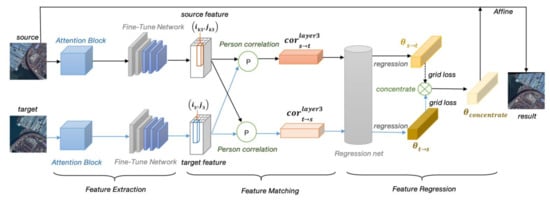
Figure 1.
Diagram showing the structure of the algorithm described in this study.
Feature extraction: This study proposes a new feature extraction structure: the combination of an attention module and a pre-training network. Firstly, the image is inputted into the attention module, and the saliency region is extracted. Then the pre-training model transfers the knowledge learned from the source domain to the target domain, which can focus on specific datasets to obtain rich and accurate feature points.
Feature matching: We make the relationship from the source feature S to the target feature T and make the relationship from the target feature T to the source feature S, finding the corresponding geometrical spatial position relation between the source image and the target image. We therefore do not rely on one-direction matching and instead use both sides to make the match, thereby avoiding the unilateral matching error and improving matching accuracy. The features of the source image and target image are extracted from the third layer of the pre-training network for Pearson correlation modeling (circled P in Figure 1), then the correlation is for bidirectional matching. Finally, the obtained relationship is inputted into the regression network.
Parameter regression: We input the two-way relationship of feature matching into a regression network for parameters regression, and thereby obtain the two parameters and ( is expressed as regressing from the source image to the target image, is expressed as regressing from the target image to the source image). Finally, the two parameters are weighted to synthesize the last parameter .
The final registration result: Geometric affine transformation is performed on the source image using the synthetic parameter .
This study will discuss the above four aspects in turn, focusing on feature extraction, feature matching, and parameter regression.
2.1. Improved Feature Extraction
The feature extraction structure designed in this study mainly consists of two parts. The first part uses the attention module composed of the channel attention mechanism and the spatial attention mechanism to detect the significance region, and the second part uses the Resnet-101 [33] pre-training network (trained in ImageNet) to extract features.
In the first part, the attention mechanism is introduced to filter out a lot of irrelevant information from top to bottom and improves the ability of feature extraction. Meanwhile, the memory structure of a neural network can be optimized to improve the capacity of a neural network to store information. The attention module basically includes four parts: a channel attention mechanism, a spatial attention mechanism, a residual structure, and a cyclic structure: (1) The channel attention mechanism is used to learn the dependence degree of each channel and adjust the different feature maps according to the dependence degree, enhancing the most informative features and suppressing useless features. (2) The spatial information in the original picture is transformed into another picture through the spatial attention mechanism and the key information is retained to find out the areas that need to be paid attention to in the picture. (3) At the same time, the residual structure is introduced into the attention module, as shown in the yellow jump connection structure and the green circle in Figure 2. Due to insufficient information after paying attention to the saliency region, the number of network layers cannot be deepened. To avoid this, the feature tensor can be combined with the feature tensor after the attention mechanism to obtain more abundant key features. (4) Considering the accuracy of extraction of key regions, the circular structure is used to re-enter the attention mechanism for extraction to further improve the ability to capture key regions.
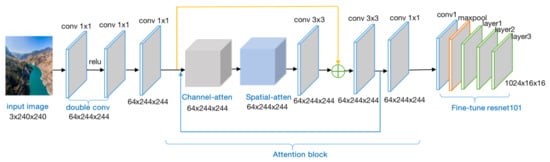
Figure 2.
Structure diagram of the feature extraction method proposed in this study.
In the second part, the model parameters of Resnet-101 trained on ImageNet are transferred to our model to help training. In this study, the structure information of the first few layers of Resnet is frozen, the following full connection layer is removed, and the remaining convolutional layer is trained for feature extraction.
Figure 2 depicts the convolution kernel size of each convolution layer, the output image size, and the channel number of each layer in the improved feature extraction section.
2.1.1. Channel Attention Mechanism
Considering the dependence of input images on each channel, the network can selectively enhance the features of a large amount of information, so that the subsequent processing can make full use of these features and suppress useless features. The channel attention mechanism is used to improve the representation capability of the network by modeling the dependencies of each channel.
The channel attention mechanism selected in this study firstly uses global pooling to generate statistics for each channel and then constructs two fully connected layers to model the correlation between channels, with the same number of weights for output and input features. Then the normalized weights between 0 and 1 are obtained through the gate of the Sigmoid activation function and weighted to the features of each channel. The output depends on the dependency of each channel. The structure is shown in Figure 3.
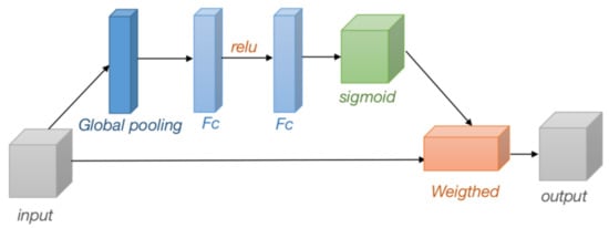
Figure 3.
Structure of channel attention module.
2.1.2. Improved Spatial Attention Mechanism
The initial spatial attention mechanism comes from the spatial transformation module proposed by Max, as shown in Figure 4. The spatial attention module is composed of a location net, grid generator, and sampler. Firstly, the important spatial regions in the image are found through the location net, and the transformation parameter is obtained by feature regression. Then the grid generator is used to find the corresponding grid points after transformation. Finally, the sampler fills in the information to get the transformed image. The main task of the location net is to find the spatial position of features through transformation and then obtain the transformation parameter . The grid generator and sampler can be thought of as a component warp, which deforms the input image according to the parameter .
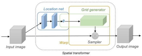
Figure 4.
Spatial transformation module.
The final output image obtained by the spatial transformation module is essentially determined by the transformation parameter . Through a series of affine transformations, such as rotation, translation, and clipping, the location net finds the saliency region adapted, obtains transformation parameters, and finally achieves the part of interest. However, a problem can appear in this process, as the output image is determined by the transformation parameters. If the transformation parameters are wrong, we will not get the ideal output image. Therefore, to enhance the accuracy of the network, Lin proposed a space transformation module of inverse synthesis for optimizing transformation parameters, as shown in Figure 5.
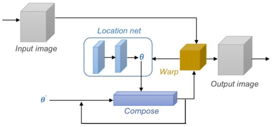
Figure 5.
Inverse synthesis of the spatial transformation module.
Different from the spatial transformation module, the inverse synthesis spatial transformation module adds two structures: (1) a cyclic structure and (2) a composite module. in Figure 5 is the prior knowledge learned by the network, which can be understood as the transformation parameters obtained by the image after it passes through the location net for the first time. When the image passes through the module the second time, the space area concerned by the network may be different, so the location net will generate a new parameter, . To focus the key areas of the image accurately, the prior parameter was combined with the new parameter to get the final required . The inverse synthesis space transformation module can provide a good foundation for subsequent operations by continuously inputting images and continuously cycling the synthesis parameters to obtain images focusing on key areas.
According to the above analysis, the spatial transformation module is used to find the key spatial regions, and the inverse synthesis of the spatial transformation module is used to accurately transform parameters and improve the ability to focus spatial positions. However, over-reliance on spatial transformation parameters may lead to focusing errors. If the prior parameters of the network have deviated, the subsequent inverse synthesis will not improve the accuracy of the transformation parameters but reduce the accuracy of the parameters. To reduce the possibility of error caused by parameters, this study inherits and improves the idea of the inverse synthesis spatial transformation module and proposes an inverse synthesis spatial transformation module with dual-vision fusion, as shown in Figure 6.
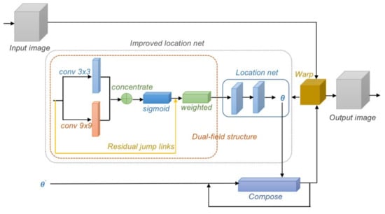
Figure 6.
Improved spatial attention module.
The orange dotted line in Figure 6 shows the dual-field attention structure proposed in this study. Images with more global information distribution prefer larger convolution kernels, while images with more local information distribution prefer smaller convolution kernels. In this study, the convolution layer with 3 × 3 and 9 × 9 convolution kernels are used to extract features from different receptive fields and the local information is fused with the global information, as shown in Figure 7. After fusion, feature maps are weighted by the sigmoid activation function and connected by a jump structure with input feature images. Finally, the attention part outputs the salient images. Compared with the original input image, the image highlights the target area, reduces the interference of other information, and lays a foundation for the location net to output transformation parameters.
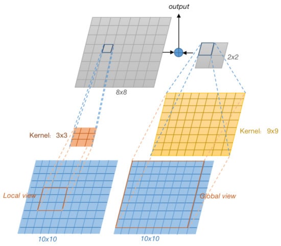
Figure 7.
Double-vision feature fusion process.
Suppose that the input image is , the characteristic image after Sigmoid activation function is , and is the parameter in the Sigmoid activation function. The calculation process of dual-field attention is shown as follows:
Formula (1) represents the fusion result of feature images in different fields after the activation function, and Formula (2) represents the output result of the weighted calculation of the fusion feature images with the original input feature images after space allocation.
2.2. Bidirectional Matching
Park once proposed that there was a matching asymmetry problem in remote sensing image registration [27], meaning that the current registration method only considers matching from the source image to the target image in one direction, lacking the matching from the target to the source in the other direction. The asymmetry of the process will lead to the degradation of the overall registration performance. We inherit the idea of double flow proposed by Park and carry out the matching from the source image to the target image and from the target image to the source image at the same time, maintaining the consistency of matching flow direction. Pearson correlation is used to construct a matching relation. The correlation between the source image and the target image is shown in Formula (3):
In the formula, represents the Pearson correlation between two feature maps with height H, width W, and channel number HW. and are the average values of the source feature graph and the target feature graph , and is the source feature vector at position . represents the target feature map after space flattening. Similarly, Pearson correlation between the target image and source image can be obtained:
where, represents the target feature vector at the position ; represents the source feature map after space flattening, ensuring that each element in the correlation vector has a corresponding mapping between the target feature and the source feature at a certain position.
2.3. Regression of Transformation Parameters
2.3.1. Loss Function
In this study, the grid loss function is used to calculate the network loss value. The formula is as follows:
In the formula, distance is the square deviation between a manually marked point on the image before transformation and a point on the output image after transformation. is the parameter of the real situation and is the output parameter after transformation. The total number of grid points is , , and the grid distance function can be regarded as an optimization problem. After training, a set of matching parameter values can be obtained.
2.3.2. Weighted Composite Parameter
Considering that the importance of bidirectional relations obtained from the matching part is the same in the matching process, both the matching relations obtained from the source image to the target image and the matching relations obtained from the target image to the source image, are mutually auxiliary in the registration process, reducing the dependence of a single relationship. Therefore, bidirectional parameters (source to target) and (target to source) obtained by the regression are synthesized in a way that is equally weighted, and the process is shown in Formula (6):
In the formula, is the final required transformation parameter, and is used to perform an affine transformation on the source image to obtain the final registration result.
3. Experiment
3.1. Training
In this study, three open multi-temporal datasets were used for evaluation, namely, Aerial Image Dataset [27], Multi Temporal Remote Sensing Registration Dataset [24], and MRSIDataset [34].
The epoch was set to 100 times, batch size to 2, lr to 0.0004, and momentum to 0.9 by using 18,000 pairs of marker transformation parameters in the Aerial Image Dataset for training. At the same time, 500 pairs of images were used for test set evaluation to verify the effect of network learning. The registration effect is verified not only on the Aerial Image Dataset but also on the Multi Temporal Remote Sensing Registration Dataset and MRSIDataset.
The experiment used Python to compile data. The experimental environment is Python 3.6, using the Pytorch framework. The hardware environment is GTX 1080 Ti graphics card, Intel® Core™ I7-7700K CPU @ 4.20 GHz processor, and 8G memory.
3.2. Comparison Algorithm
This study compares five remote sensing image registration algorithms containing two classical algorithms, ORB [19] and SIFT [17], and three deep learning-based registration algorithms developed in recent years—CNNGeo [31], Multi-time Registration [24], and Two-stream Ensemble [27]. At the same time, the model based on deep learning was retrained on the dataset in this study, and the parameter settings were the same as our experimental settings.
3.3. Evaluation
To verify the experimental effect of this study, Checkboard and Overlap qualitative evaluations were used to evaluate the registration effect, and seven evaluation methods, consisting of PCK [35], Loss, RMSE (Root Mean Square Error), SSIM (Structural Similarity Index) [36], NCC (Normalized Cross Correlation), Entropy, and Run time, were used to evaluate the registration quantitative effect of the model.
Checkboard: Dividing the target image and the registration result into several squares, each square appears alternately. Then, observing the alignment of each square junction, if it can be aligned, the registration effect is deemed good.
Overlap: Checkboard observes the local registration of images from details, while Overlap observes the registration of two images from the whole. If there is a large registration error between images, there will be fuzzy and disorderly situations on the Overlap.
PCK: Evaluates the probability of successful matching of correct key points between two images. The formula is as follows:
Formula (7) represents the ratio of the number of correctly detected key points to the number of marked keys. N represents the total number of images, represents the final transformation parameter, is the source key point obtained by the transformation of the ith image pair, is the manually marked key point in the ith image pair, and represents the maximum threshold range. Among them, in the picture with height h and width w, if is larger (the coefficient does not exceed 1) and the threshold range is larger, the registration situation can be measured globally. Generally speaking, 0.05 is more appropriate for . The higher the value of this indicator, the higher the registration accuracy.
Loss: Contain train loss and test loss. Train loss represents the loss in the process of model training. Test loss verifies the design structure and the overall effect of the model. If both train loss and test loss show an overall downward trend, it is indicated that the model design is reasonable. The smaller the loss value, the faster the gradient descent, and the better the model convergence effect.
RMSE: Represents the deviation between the target image and the image after registration. The smaller the RMSE value, the better the effect. The formula is as follows:
In the formula, N represents pixel points in the image, is pixel points obtained from the image after registration, and is pixel points marked on the target image.
SSIM: The similarity is measured by comparing the brightness, contrast, and structure between the target image and the registered image. The larger the SSIM value, the stronger the structural similarity between images, and the better the registration result.
where is brightness similarity, is contrast similarity, and is structure similarity. are the three similarity parameters; makes the expression simpler.
NCC: This is used to normalize the degree of correlation between targets to be matched. By searching an image for the region with the highest NCC and taking a little known region as a corresponding match, the whole image is aligned. The larger the NCC value, the more similar the two vectors will be, and the better the matching performance between images.
where represents the target image and represents the image after registration.
Entropy: Indicates the degree of dispersion in the spatial distribution of key points. The higher the information entropy value, the higher the distribution of the key point’s dispersion degree; and the more accurate the transformation parameters calculated by the registration point, the better the registration effect will be.
In the formula, is the set of registration points, and , represents the gaussian function value of the distance between point p and all points in .
Run time: The faster the model runs, the greater the efficiency, and the more feasible it will prove to be in practical applications.
3.4. Experimental Results in Practical Application
In this study, registrations were tested on three datasets, namely, the Aerial Image Dataset, the Multi Temporal Remote Sensing Registration Dataset, and MRSIDataset, as shown in Figure 8, Figure 9 and Figure 10.
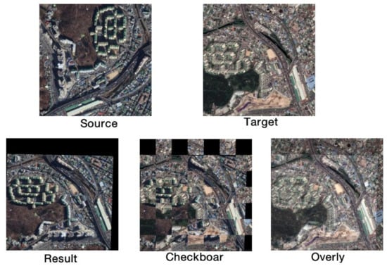
Figure 8.
Multi-temporal city image registration results from the Aerial Image Dataset.
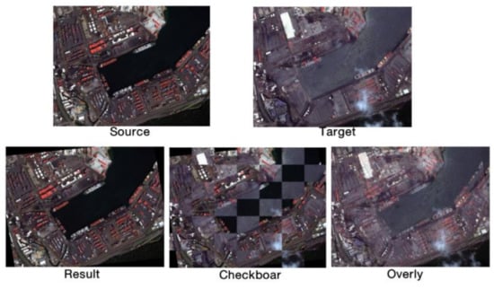
Figure 9.
Multi-temporal port image registration results from MRSIDataset.
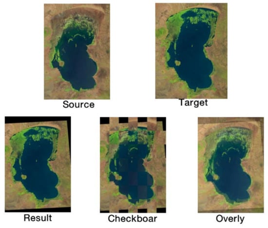
Figure 10.
Multi-temporal Remote Sensing Registration Dataset for lake image registration.
Figure 8 shows a group of multi-temporal urban remote sensing images from the Aerial Image Dataset. The study of multi-temporal urban remote sensing images can effectively observe the urban change dynamics, land coverage rate, and spatial pattern change. Remote sensing registration technology is used to observe the changes of green land cover, construction land, water area land, and farmland, to provide a scientific basis for the ecological planning and construction of the urban landscape. The source image and the target image were taken at different times in the same place. By registering the source image to the target image, the result can keep the road and built-up area aligned. The registration result shows that the land used for buildings is larger than before, while the vacant land is transformed into green plant cover, and the road direction remains unchanged. It provides an analytical basis for future urban construction trends in this region.
The multi-temporal image pair from MRSIDataset in Figure 9 is a set of coastal ports taken during the day and at night. As can be seen from Figure 9, the registration focuses align with the port boundary area and the boundary area matches. It can be observed that there are more ships in the harbor during the day and fewer ships at night. Even with cloud interference, there is little influence on registration.
Figure 10 shows an image from the Multi Temporal Remote Sensing Registration Dataset—a pair of multi-temporal images of lakes. According to the registration results, the two images are aligned. Changes in the lake area and vegetation coverage are observed by both checkboard and Overly. How to establish the relationship between landscape spatial pattern and ecological environment function is a problem that needs to be considered after studying land utilization rate change.
3.5. Contrast Experiments
3.5.1. Aerial Image Dataset
Three groups of registration images were selected from the Aerial Image Dataset for comparing the performance of the algorithms. Figure 11, Figure 12 and Figure 13 show the multi-temporal urban registration results, multi-temporal rural registration results, and multi-temporal island registration results are presented, respectively. The two images at the top of each group are the source image and the target image. The Overly results are used to observe the overall registration, and the Checkboard results are used to observe the local detail registration. By comparing the registration results in this study, the algorithm in this paper can be seen to have the highest registration accuracy compared to the other five algorithms.
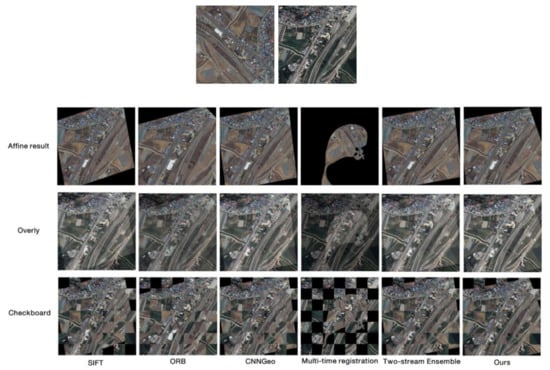
Figure 11.
Comparison map of urban qualitative registration of six methods on the Aerial Image Dataset.
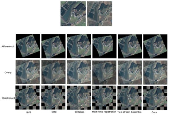
Figure 12.
Comparison map of rural qualitative registration of six methods on the Aerial Image Dataset.
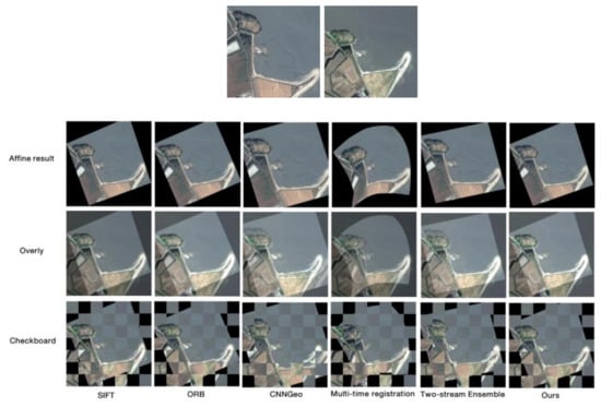
Figure 13.
Comparison map of island qualitative registration with six methods on the Aerial Image Dataset.
Meanwhile, RMSE, SSIM, and NCC are used to evaluate the accuracy of the above images, as shown in Table 1, Table 2 and Table 3.

Table 1.
Evaluation of the first group of images on the Aerial Image Dataset.
Table 2.
Evaluation of the second group of images on the Aerial Image Dataset.
Table 3.
Evaluation of the third group of images on the Aerial Image Dataset.
Black data in the table is the optimal data. By looking at the information in the table, it can be seen that the method in this study always achieves the best accuracy effect on the Aerial Image Dataset. RMSE has the lowest registration error, SSIM has the highest matching similarity, and NCC has the highest correlation between two images, indicating that the method in this study has superior registration accuracy performance.
3.5.2. MRSIDataset
The images in Figure 14, Figure 15 and Figure 16 are from the multi-temporal dataset MRSIDataset, and show a desert oasis map, a river map, and a city map respectively. Affine results, Overly, and Checkboard registration results show that the proposed method obtains the best registration effect, not only achieving global alignment but also matching the target image in detail (roads, rivers, etc.).
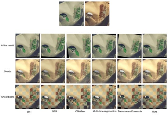
Figure 14.
Comparison map of qualitative registration of desert oases using six methods on MRSIDataset.
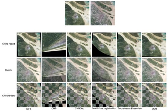
Figure 15.
Comparison map of river qualitative registration with six methods on MRSIDataset.
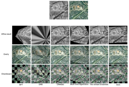
Figure 16.
Comparison map of six methods for urban qualitative registration on MRSIDataset.
RMSE, SSIM, and NCC are also used for quantitative evaluation of the six methods, as shown in Table 4, Table 5 and Table 6. Black data marked in the table is the optimal data, as shown in the table. Compared with the other five methods, the method developed in this paper has an excellent performance with respect to the MRSIDataset test images, achieving the highest accuracy.
Table 4.
Evaluation of the first group of images on MRSIDataset.
Table 5.
Evaluation of the second group of images on MRSIDataset.
Table 6.
Evaluation of the third group of images on MRSIDataset.
3.5.3. Multi Temporal Remote Sensing Registration Dataset
The multi-temporal matching image pairs shown in Figure 17, Figure 18 and Figure 19 are taken from the Multi Temporal Remote Sensing Registration Dataset. The image pairs shown in this study are the comparison results for valley slits, mountains, rivers, and lakes. Compared with the other five methods, it is observed that the proposed method has better registration results.
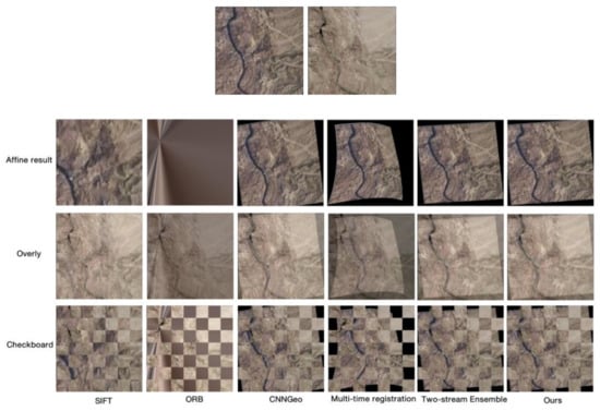
Figure 17.
Comparison diagram of six methods for qualitative registration of slit on the Multi Temporal Remote Sensing Registration Dataset.
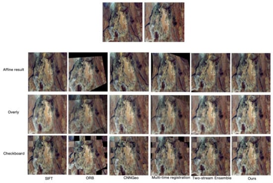
Figure 18.
Comparison diagram of mountain and river qualitative registration with six methods on the Multi Temporal Remote Sensing Registration Dataset.
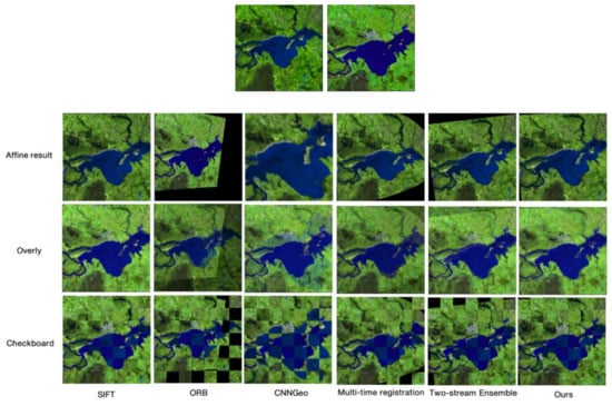
Figure 19.
Comparison diagram of lake qualitative registration with six methods on the Multi Temporal Remote Sensing Registration Dataset.
Evaluation indicators are used to quantitatively evaluate the images shown in the Multi Temporal Remote Sensing Registration Dataset, as shown in Table 7, Table 8 and Table 9. Compared with the other five methods, the proposed method is optimal with respect to RMSE, SSIM, and NCC, and the model has the highest accuracy and the best registration effect.
Table 7.
Evaluation of the first group of images on the Multi Temporal Remote Sensing Registration Dataset.
Table 8.
Evaluation of the second group of images on the Multi Temporal Remote Sensing Registration Dataset.
Table 9.
Evaluation of the third group of images on the Multi Temporal Remote Sensing Registration Dataset.
3.5.4. Assessment of the Three Datasets
A time efficiency evaluation was performed on the three datasets above, as shown in Figure 20. The abscissa is tested by the three groups of multi-temporal image pairs from the Aerial Image Dataset, and the ordinate is the running time in seconds. The six methods of comparison are represented by bars of different colors. As can be seen from Figure 20, the running time of the method in this study is much lower than that of the Multi-time Registration method, and it runs more efficiently than the other methods. Additionally, in relation to CNNGeo and the Two-stream Ensemble, our method design, using an end-to-end pre-trained model, when it is compared with the model without pre-training, shows a faster training rate and higher running efficiency.
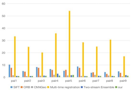
Figure 20.
Time contrast diagram.
In this study, not only does the accuracy index measure the correlation between the registration error and the registration results, but also the Entropy index is used to measure the information of the registration results, which can reflect the degree of dispersion of the registration points in the image spatial distribution. The higher the degree of dispersion, the more accurate the transformation parameters obtained by the model. In Figure 21, the method proposed (shown in the green broken line) is always at the top. This indicates that the Entropy value of the proposed method is the highest in the measured image, that is, it shows the method to have the highest accuracy.
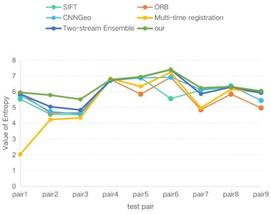
Figure 21.
Entropy contrast diagram.
3.5.5. Ablation Experiments
Our contributions in this paper can be divided into two main parts: (1) feature extraction: a new feature extraction framework called improved extraction is proposed to improve the attention mechanism and the structure of the network; (2) feature matching: we proposed a bidirectional matching algorithm. Pearson correlation is used to improve the cross-correlation and a bidirectional matching network is built to ensure the symmetry of the network and reduce the dependence on single matching. Ablation experiments are conducted to prove the effectiveness of our methods. In this work, CNNGeo is selected as the basic registration network framework. The pre-trained resnet101 model is used for feature extraction, and the one-way cross-correlation is used for feature matching. A final parameter can be obtained by the regression step for the transformation operation in the stage of registration. The Two-stream Ensemble network uses pre-trained SE-resnext101 with an attention mechanism for feature extraction and a bidirectional two-stream network for matching. This is a novel registration method that has been proposed in recent years. In this paper, the two proposed components are respectively added to the CNNGeo infrastructure to calculate the change in the PCK value. Finally, it is compared with the PCK value of the Two-stream Ensemble model to evaluate the overall accuracy of our model. The three network models are trained with 18,000 image pairs from the Aerial Image Dataset and tested on 500 pairs test set for the PCK metric. The test results are shown in Table 10, below.
Table 10.
Ablation quantitative analysis table.
As shown in Table 10, the performance of the CNNGeo model with the addition of the two components we have proposed is significantly improved. Moreover, the PCK accuracy of our method is higher than that of the Two-stream Ensemble method and has a high registration accuracy. In addition, the loss diagram is used to show the training and testing process of the Two-stream Ensemble model and the model described in this paper, as shown in Figure 22 and Figure 23.
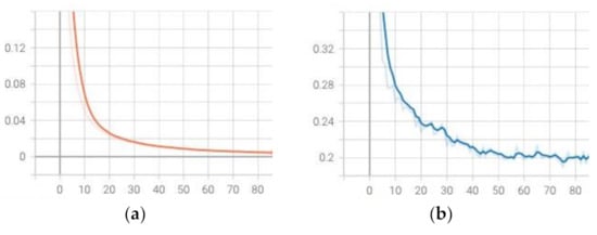
Figure 22.
(a) shows the training loss diagram of the algorithm described in this paper. (b) shows the test loss diagram of the algorithm.
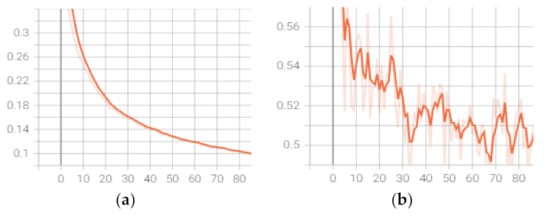
Figure 23.
(a) is the training loss diagram of the Two-stream Ensemble method. (b) is the test loss diagram of the Two-stream Ensemble.
It can be seen from Figure 22 and Figure 23 that the overall loss of the proposed method in this paper shows a gentle downward trend, while the Two-stream Ensemble model shows a downward trend, but one which shows the training process to fluctuate greatly, it being not as gentle as the trend generated by the method proposed in this paper. Additionally, the training loss and test loss values for our method are lower than the loss values for the Two-stream Ensemble method. This implies that the training process of our method is the better one, and the loss is smaller.
4. Discussion
4.1. Discussion of Application
We evaluated our proposed method using a variety of datasets. Figure 24 and Figure 25 showed that our method correctly aligned the multimodal image pairs from RMSIDatasets and yielded accurate matching results.
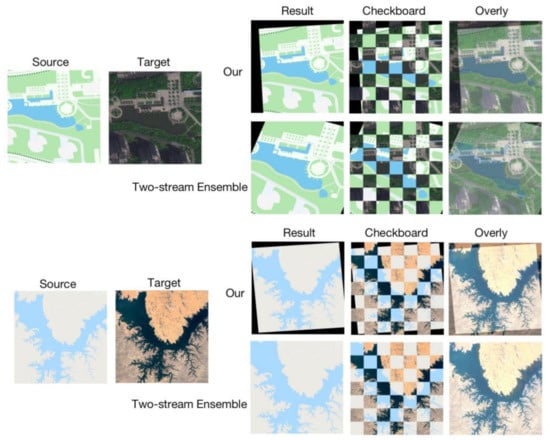
Figure 24.
Map-optical registration image.
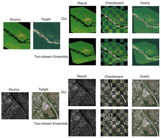
Figure 25.
SAR-optical registration image.
The image in Figure 24 is a map-optical registration and Figure 25 is an SAR optical registration. We compare the proposed method with the Two-stream Ensemble method. The experimental results show that our method has accurate matching results on multi-temporal datasets and has greater expansion on other datasets. To summarize, the proposed method improves the precision of registration and maintains the strong robustness of deep-learning methods at the same time. Additionally, it has strong practicability and a wide scope of application.
4.2. Limitations
In the process of image registration, a certain gap between the shooting angle and the acquisition of the image has appeared. Therefore, the consideration of a single type of image registration may lead to errors in the results and limitations in terms of practical applications. The algorithm presented in this paper has registration biases for multi-temporal images with relatively different viewing angles, as shown in Figure 26. The images were taken from multi-temporal image pairs with significant angle changes.
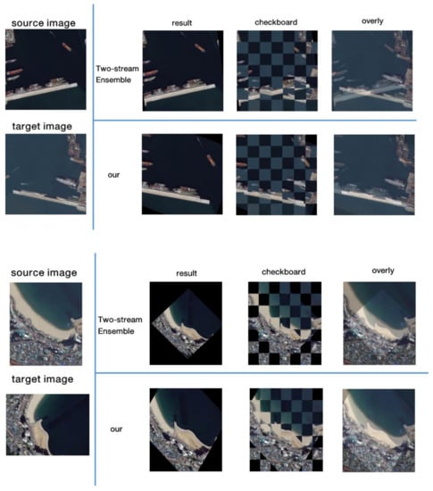
Figure 26.
Results of multi-time image registration with obvious angle change.
The proposed algorithm can accurately align multi-temporal image pairs with small angle differences, but there are still limitations for image pairs with large angle differences. These problems raised by image registration will lead to limitations in the use of the algorithm, which will be subject to further improvements in the future.
4.3. Future Directions
We aim to expand the scope of application of the model in the future. In the field of actual remote sensing image registration, the image information is complex and there may be differences between the image acquisition source or photographing angle and capture. Therefore, for multi-temporal image registration, although the time difference is the dominant factor, there will inevitably be an angle difference. Consequently, a more standardized network model is needed to register such complex images in order to widen the field of practical applications.
5. Conclusions
In this paper, a bidirectional symmetry registration network with a dual field of view circulation is proposed, aiming at the problems of feature extraction and feature matching. The proposed framework combines an attention module and transfer learning for the purpose of feature extraction. Combined with the idea of local and global feature extraction, a parallel dual view of the spatial attention module is constructed. At the same time, the loop mechanism is used to improve the network structure. The matching structure with bidirectional symmetry is designed to reduce the matching error caused by the unidirectional matching structure. The bidirectional parameters of regression are synthesized to obtain the final more accurate transformation parameters for registration. Experimental results show that our proposed method has strong accuracy on three public datasets, and the accuracy and efficiency of the algorithm are better than the two classical methods and the three methods proposed in recent years. Consequently, the method we have here described can enhance the matching accuracy and improve the precision of registration.
In future research, we will look to enhance the applicability of the method and improve its generalization. It is a method that can handle complex conditions with large amounts of variation in images and promises to solve a number of image registration problems in practical contexts, saving resources and improving efficiency.
Author Contributions
The contributions of the authors are as follows: study design, Q.Z. and Y.C.; data collection, Q.Z.; data analysis, Q.Z.; writing—original draft preparation, Q.Z. and W.Z.; writing—review and editing, Q.Z., L.C. and W.Z.; literature search, Q.Z.; figures, Q.Z. and L.C.; final approval Y.C. All authors have read and agreed to the published version of the manuscript.
Funding
This research was funded by the National Natural Science Foundation of China, grant number 61976140, and the Collaborative Innovation Foundation of Shanghai Institute of Technology, grant number XTCX2018-17.
Acknowledgments
The authors would like to thank the anonymous reviewers for their constructive comments.
Conflicts of Interest
The authors declare no conflict of interest.
References
- Sidike, P.; Prince, D.; Essa, A.; Asari, V.K. Automatic building change detection through adaptive local textural features and sequential background removal. In Proceedings of the 2016 IEEE International Geoscience and Remote Sensing Symposium (IGARSS), Beijing, China, 1 July 2016; pp. 2857–2860. [Google Scholar]
- Crisp, D.J. A ship detection system for RADARSAT-2 dual-pol multi-look imagery implemented in the ADSS. In Proceedings of the 2013 IEEE International Conference on Radar, Adelaide, Australia, 9–12 September 2013; pp. 318–323. [Google Scholar]
- Wang, C.; Bi, F.; Zhang, W.; Chen, L. An intensity-space domain cfar method for ship detection in HR SAR images. IEEE Geosci. Remote Sens. Lett. 2017, 14, 529–533. [Google Scholar] [CrossRef]
- Leng, X.; Ji, K.; Zhou, S.; Xing, X.; Zou, H. An adaptive ship detection scheme for spaceborne SAR imagery. Sensors 2016, 16, 1345. [Google Scholar] [CrossRef] [PubMed] [Green Version]
- Liu, J.; Geng, Y.; Zhao, J.; Zhang, K.; Li, W. Image semantic segmentation use multiple-threshold probabilistic R-CNN with feature fusion. Symmetry 2021, 13, 207. [Google Scholar] [CrossRef]
- Wang, S.; Sun, X.; Liu, P.; Xu, K.; Zhang, W.; Wu, C. Research on remote sensing image matching with special texture background. Symmetry 2021, 13, 1380. [Google Scholar] [CrossRef]
- Zeng, Y.; Ning, Z.; Liu, P.; Luo, P.; Zhang, Y.; He, G. A mosaic method for multi-temporal data registration by using convo-lutional neural networks for forestry remote sensing applications. Computing 2020, 102, 795–811. [Google Scholar] [CrossRef]
- Chen, J.; Chen, S.; Liu, Y.; Chen, X.; Yang, Y.; Zhang, Y. Robust local structure visualization for remote sensing image registration. IEEE J. Sel. Top. Appl. Earth Obs. Remote Sens. 2021, 14, 1895–1908. [Google Scholar] [CrossRef]
- Wang, D.; Chen, Y.; Li, J. Remote sensing image registration based on full convolution neural network and k-nearest neighbor ratio algorithm. J. Phys. Conf. Ser. 2021, 1873, 012026. [Google Scholar] [CrossRef]
- Liang, L.; He, Q.; Cao, H.; Yang, Y.; Chen, X.; Lin, G.; Han, M. Dual-features student-t distribution mixture model based remote sensing image registration. IEEE Geosci. Remote Sens. Lett. 2021, 1–5. [Google Scholar] [CrossRef]
- Tondewad, M.P.S.; Dale, M. remote sensing image registration methodology: Review and discussion. Procedia Comput. Sci. 2020, 171, 2390–2399. [Google Scholar] [CrossRef]
- Ye, Z.; Kang, J.; Yao, J.; Song, W.; Liu, S.; Luo, X.; Xu, Y.; Tong, X. Robust fine registration of multisensor remote sensing images based on enhanced subpixel phase correlation. Sensors 2020, 20, 4338. [Google Scholar] [CrossRef] [PubMed]
- Rahaghi, A.I.; Lemmin, U.; Sage, D.; Barry, D.A. Achieving high-resolution thermal imagery in low-contrast lake surface waters by aerial remote sensing and image registration. Remote Sens. Environ. 2019, 221, 773–783. [Google Scholar] [CrossRef]
- Li, Q.; Han, G.; Liu, P.; Yang, H.; Luo, H.; Wu, J. An infrared-visible image registration method based on the constrained point feature. Sensors 2021, 21, 1188. [Google Scholar] [CrossRef] [PubMed]
- Dong, Y.; Jiao, W.; Long, T.; Liu, L.; He, G. Eliminating the effect of image border with image periodic decomposition for phase correlation based remote sensing image registration. Sensors 2019, 19, 2329. [Google Scholar] [CrossRef] [PubMed] [Green Version]
- Ye, Y.; Wang, M.; Hao, S.; Zhu, Q. A novel keypoint detector combining corners and blobs for remote sensing image registration. IEEE Geosci. Remote. Sens. Letters. 2020, 18, 451–455. [Google Scholar] [CrossRef]
- Lowe, D.G. Distinctive image features from scale-invariant key points. Int. J. Comput. Vis. 2004, 60, 91–110. [Google Scholar] [CrossRef]
- Bay, H.; Ess, A.; Tuytelaars, T.; Van Gool, L. Speeded-Up Robust Features (SURF). Comput. Vis. Image Underst. 2008, 110, 346–359. [Google Scholar] [CrossRef]
- Rublee, E.; Rabaud, V.; Konolige, K.; Bradski, G.R. ORB: An efficient alternative to SIFT or SURF. In Proceedings of the IEEE International Conference on Computer Vision, ICCV 2011, Barcelona, Spain, 6–13 November 2011; pp. 2564–2571. [Google Scholar]
- Kou, Q.; Cheng, D.; Chen, L.; Zhao, K. A multiresolution gray-scale and rotation invariant descriptor for texture classification. IEEE Access 2018, 6, 30691–30701. [Google Scholar] [CrossRef]
- Harris, C.G.; Stephens, M.J. A combined corner and edge detector. In Proceedings of the 4th Alvey Vision Conference, Manchester, UK, 31 August–2 September 1988; pp. 147–151. [Google Scholar]
- He, X.; Yung, N. Curvature scale space corner detector with adaptive threshold and dynamic region of support. In Proceedings of the 17th International Conference on Pattern Recognition, Cambridge, UK, 26–26 August 2004; Volume 2, pp. 791–794. [Google Scholar]
- Dou, Q.; Shuang, W.; Ning, M.; Tao, X.; Jiao, L. Using deep neural networks for synthetic aperture radar image registration. In Proceedings of the IEEE International Geoscience and Remote Sensing Symposium (IGARSS), Yokohama, Japan, 28 July 2016; pp. 2799–2802. [Google Scholar]
- Yang, Z.; Dan, T.; Yang, Y. Multi-temporal remote sensing image registration using deep convolutional features. IEEE Access 2018, 6, 38544–38555. [Google Scholar] [CrossRef]
- Ye, F.; Su, Y.; Xiao, H.; Zhao, X.; Min, W. Remote sensing image registration using convolutional neural network features. IEEE Geosci. Remote Sens. Lett. 2018, 15, 232–236. [Google Scholar] [CrossRef]
- Kim, D.-G.; Nam, W.-J.; Lee, S.-W. A robust matching network for gradually estimating geometric transformation on remote sensing imagery. In Proceedings of the 2019 IEEE International Conference on Systems, Man and Cybernetics (SMC), Bari, Italy, 6 October 2019; pp. 3889–3894. [Google Scholar]
- Park, J.-H.; Nam, W.-J.; Lee, S.-W. A two-stream symmetric network with bidirectional ensemble for aerial image matching. Remote Sens. 2020, 12, 465. [Google Scholar] [CrossRef] [Green Version]
- Lin, C.H.; Lucey, S. Inverse compositional spatial transformer networks. In Proceedings of the 2017 IEEE Conference on Computer Vision and Pattern Recognition (CVPR), Honolulu, HI, USA, 21–26 July 2017; pp. 2568–2576. [Google Scholar]
- Max, J.; Karen, S.; Andrew, Z.; Koray, K. Spatial transformer networks. In Proceedings of the Advances in Neural Information Processing Systems (NIPS), Montréal, QC, Canada, 7 December 2015; pp. 2017–2025. [Google Scholar]
- Marcu, A.; Leordeanu, M. Dual local-global contextual pathways for recognition in aerial imagery. arXiv 2016, arXiv:1605.05462. [Google Scholar]
- Rocco, I.; Arandjelovic, R.; Sivic, J. Convolutional neural network architecture for geometric matching. In Proceedings of the IEEE Conference on Computer Vision and Pattern Recognition (CVPR), Honolulu, HI, USA, 21–26 July 2017. [Google Scholar]
- Kim, B.; Kim, J.; Lee, J.G.; Dong, H.K.; Ye, J.C. Unsupervised deformable image registration using cycle-consistent CNN. In Proceeding of the International Conference on Medical Image Computing and Computer-Assisted Intervention (MICCAI), Shenzhen, China, 13 October 2019; pp. 166–174. [Google Scholar]
- He, K.; Zhang, X.; Ren, S.; Sun, J. Identity mappings in deep residual networks. In Lecture Notes in Computer Science, Proceedings of the 14th European Conference, Amsterdam, The Netherlands, 11–14 October 2016; Springer Nature: Basingstoke, UK, 2016; Volume 9908, pp. 630–645. [Google Scholar]
- Li, J.; Hu, Q.; Ai, M. RIFT: Multi-modal image matching based on radiation-variation insensitive feature transform. IEEE Trans. Image Process. 2019, 29, 3296–3310. [Google Scholar] [CrossRef] [PubMed]
- Sun, X.; Xiao, B.; Wei, F.; Liang, S.; Wei, Y. Integral human pose regression. Comput. Sci. 2018, 11210, 536–553. [Google Scholar]
- Wang, Z.; Bovik, A.; Sheikh, H.; Simoncelli, E.P. Image quality assessment: From error visibility to structural similarity. IEEE Trans. Image Process. 2004, 13, 600–612. [Google Scholar] [CrossRef] [PubMed] [Green Version]
Publisher’s Note: MDPI stays neutral with regard to jurisdictional claims in published maps and institutional affiliations. |
© 2021 by the authors. Licensee MDPI, Basel, Switzerland. This article is an open access article distributed under the terms and conditions of the Creative Commons Attribution (CC BY) license (https://creativecommons.org/licenses/by/4.0/).